Serial versus parallel search: A model comparison approach based on reaction time distributions

ABSTRACT

For 50 years or so, visual search experiments have been used to examine how humans find behaviourally relevant objects in complex visual scenes. For the same length of time, there has been a dispute over whether this search is performed in a serial or parallel fashion. In this paper, we approach this dispute by numerically fitting a serial search model and a parallel search model to reaction time (RT) distributions from three visual search experiments (feature search, conjunction search, spatial configuration search). In order to do so, we used a free-likelihood method based on a novel kernel density estimator (KDE).

The serial search model was the Competitive Guided Search (CGS) model by Moran et al. [(2013). Competitive guided search: Meeting the challenge of benchmark RT distributions. Journal of Vision, 13(8), 24–24.]. We were able to replicate the ability of CGS to model RT distributions from visual search experiments, and demonstrated that CGS generalizes well to new data. The parallel model was based on the biased-competition theory and utilized a very simple biologically-plausible winner-take-all (WTA) mechanism from Heinke and Humphreys’s [(2003). Attention, spatial representation and visual neglect: Simulating emergent attention and spatial memory in the Selective Attention for Identification Model (SAIM). Psychological Review, 110(1), 29–87.]. With this mechanism, SAIM has been able to explain a broad range of attentional phenomena but it was not specifically designed to model RT distributions in visual search. Nevertheless, the WTA was able to reproduce these distributions.

However, a direct comparison of the two models suggested that the serial CGS is slightly better equipped to explain the RT distributions than the WTA mechanism. The CGS’s success was mainly down the usage of the Wald distribution which was specifically designed to model visual search. Future WTA versions will have to find a biologically plausible mechanism to reproduce such a RT distribution. Finally, both models suffered from a failure to generalize across all display sizes. From these comparisons, we developed suggestions for improving the models and motivated empirical studies to devise a stronger test for the two types of searches.

KEYWORDS:

• Computational modelling
• visual search
• biased competition
• RT distribution
• kernel density estimator

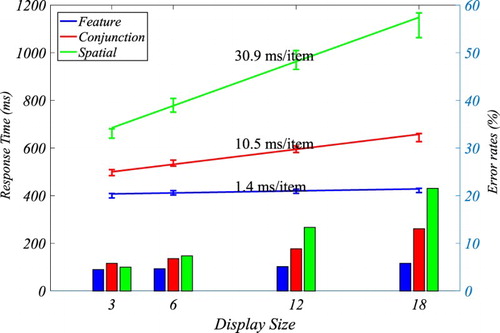
For the last 50 years or so the visual search task has been a commonly used experimental procedure to study human processing of multiple object scenes (see Eckstein, 2011, for a review). In a standard visual search task, participants are asked to determine whether a predefined target item among non-targets (distractors) on a computer screen is present or absent. During the course of the experiments, the number of distractors (display size) is varied. Typically, the time it takes participants to make this decision (reaction time; RT) is measured as a function of the display size (search function). The slope of the search function is interpreted as an indicator of the search efficiency for particular target–distractor pairings. Slopes can range from close to 0 ms/item (highly efficient) to larger than 30 ms/item (highly inefficient).

Examples of highly efficient searches are the search for a tilted line among vertical lines (Treisman & Gormican, 1988) or for a red among green circles (Egeth, Jonides, & Wall, 1972). These searches are usually termed “feature searches” as the target can be distinguished on the basis of a single feature, e.g., orientation or colour. A classic example of an inefficient search is when target and distractor need to be determined based on local features within items (“spatial configuration”) e.g., letter T among Ls (Kwak, Dagenbach, & Egeth, 1991). Somewhat intermediate efficient searches can often be found in “conjunction searches” where targets and distractors have to be distinguished on the basis of the combination of two or more features, e.g., a search for a vertical red bar among horizontal red bars and vertical green bars (Wolfe, Cave, & Franzel, 1989).

From the beginning of research into visual search the results have been discussed in terms of the dichotomy of parallel vs. serial search (Treisman & Gelade, 1980). In broad terms, serial search assumes that items in a search display are attended to one by one and each examined as to whether it constitutes the target. In parallel search, all items are examined in parallel as to whether they are the target. Moreover, search results with a shallow slope have been considered to be parallel searches while steeper slopes are interpreted as evidence for serial search. However, it can be shown that mean RTs and slopes are not sufficient to distinguish between serial versus parallel processing as both types of searches are able to produce efficient or inefficient searches (Townsend & Ashby, 1984; Townsend & Nozawa, 1995). A potential solution for this inability to make this decision may be to consider RT distributions as they would contain more information about the underlying search type (Balota & Yap, 2011; Ratcliff, 1978; Wolfe, Palmer, & Horowitz, 2010). This paper will fit two computational models to RT distributions. The two models implement the two types of search. We will evaluate which of the two models explains better the two types of search and consequently this model comparison will allow us to decide which search strategy was most likely employed in the given data. At this point it is worth stressing that this paper focuses on the dichotomy of parallel vs. serial rather than on how visual features, such as colour or orientation, influence visual search. In other words, such perceptual features in this framework turn into free model parameters rather than explicit computations.

Probably the most influential serial search theory is “Guided Search” by Wolfe and colleagues (Wolfe, 1994, 2007; Wolfe et al., 1989). Guided Search posits a two-stage architecture. The first stage is a parallel processing stage and determines a saliency map of a visual scene (Koch & Ullman, 1985). This saliency map indicates the conspicuity of items in terms of how distinct the perceptual properties of an item are compared to other items’ perceptual properties (see Bruce & Tsotsos, 2009; Itti, Koch, & Niebur, 1998, for examples of computational models of saliency maps). The saliency map guides the serial search process in the second stage. This guidance directs the search along decreasing item saliencies. This way Guided Search can explain highly efficient searches such as feature searches, where targets are highly salient. For highly inefficient searches, such as the spatial configuration task, target items are assumed to be not salient leading to a lack of guidance. Consequently, search becomes random. Note, however, that Guided Search also assumes that serial search is not only guided by such perceptual (i.e., bottom-up) factors but also by top-down factors such as knowledge about the target itself (Wolfe, 1998). This way searches like spatial configuration search may be not entirely random.

A recent paper by Moran, Zehetleitner, Mueller, and Usher (2013) numerically fitted an instantiation of the Guided Search theory, termed Competitive Guided Search (CGS), to RT distributions from visual experiments. The data was taken from Wolfe et al.’s (2010) data set which includes results from the three standard tasks: a feature search (red vertical bar among green vertical bars), a conjunction search (red vertical bar among green vertical bars and red horizontal bars) and a spatial configuration search (2 among 5s). They demonstrated that their model can successfully reproduce RT distributions from these search tasks. Based on their success we will use CGS as a reference model to a parallel search model. Moreover, Moran et al. (2013) used the best fitting distribution for Wolfe et al.’s (2010) data, Wald distribution (Palmer, Horowitz, Torralba, & Wolfe, 2011) as basis for CGS’s identification stage (see below for details). Hence, it is questionable whether CGS generalizes to other data. We will therefore test CGS with our own data (Lin, Heinke, & Humphreys, 2015).

Probably the most influential parallel search theory is the Biased Competition Theory (Desimone & Duncan, 1995; Duncan, Humphreys, & Ward, 1997). This theory suggests that search items compete for response, and that reaction times and search efficiencies depend on the “amount” of interference between items during this competition. Analogous to Guided Search, the competition process is assumed to be affected by bottom-up and top-down factors (e.g., expectations about targets, Anderson, Heinke, & Humphreys, 2010; or short-term memory, Woodgate, Strauss, Sami, & Heinke, 2015). Several computational modelling studies have found that indeed parallel competition between items can explain search efficiency, most prominently the Selective Attention for Identification Model (SAIM; Heinke & Backhaus, 2011; Heinke & Humphreys, 2003; Mavritsaki, Heinke, Humphreys, & Deco, 2006). SAIM’s competition mechanism is able to model a broad range of empirical evidence typically associated with visual selective attention and its disorders. Its most recent instalment, VS-SAIM, was able to simulate visual search experiments (Heinke & Backhaus, 2011). However, in this study SAIM was evaluated in a qualitative way. This paper aims to rectify this shortcoming by taking SAIM’s core mechanism, a winner-take-all (WTA) network, and evaluating it quantitatively with RT distributions taken from Lin et al.’s (2015) data. It is also worth noting that Bundesen’s (1990) biased-competition model (TVA) was fitted quantitatively albeit based on mean RTs. Of course, any parallel search model is likely to represent a simplification of how visual search is implemented and a serial component is certainly part of a fuller picture. For one thing, eye movements are an obvious candidate for a serial component (see Hulleman & Olivers, 2016, on the importance of eye movements). It is also conceivable that some serial “internal rejecting” after a parallel search may take place (see SEarch via Recursive Rejection SERR, Humphreys & Müller, 1993, for an example). It is also clear that such serial components are particularly important in target-absent trials (even though perhaps not in terms of eye movements as discussed in Wolfe, 2007). Hence, we will focus in this paper on present trials. Nevertheless, previous studies with parallel-only models such as SAIM imply that such a parallel approach may go a long way in explaining visual search, particularly for target-present trials. Here, we will follow-up and utilize RT distributions to further evaluate this approach. Moreover, the direct comparison with a serial approach will give us a good insight into what may be missing in the parallel-only approach. In fact, CGS represents a particularly strong challenge as CGS is developed especially for modelling visual search while SAIM was developed to account for a broad range of attentional effects. Another argument for fitting a simple parallel model comes from the methodology issue posed by utilizing RT distributions. In this paper, we will present a novel method of fitting RT distributions. Such a novel method is better tested with simple models or models where we already know that they are successful elsewhere such as CGS.

It is well-known that obtaining veridical estimates of RT distributions is challenging and standard estimators (e.g., histograms) require thousands of trials (Van Zandt, 2000). Here we will present a novel version of the kernel density estimator (KDE) termed on-line KDE (oKDE; Kristan, Leonardis, & Skočaj, 2011) and demonstrate that oKDE is suitable to veridically represent RT distributions for around 100 trials.

The structure of this paper is as follows. We will first introduce the visual search experiments (feature search, conjunction search, spatial configuration search) from which we used the data. Then we introduce the two models and discuss them. As the biased-competition model uses the WTA mechanism from SAIM, we termed this model SAIM-WTA. In Method, we introduce the computational methods we used to fit the models. In particular, we present a novel KDE capable of representing RT distribution with extremely high accuracy using around 100 trials in each condition. The results section demonstrates that SAIM-WTA can be fitted well to the visual search data and that we are able to qualitatively replicate Moran et al.’s (2013) fits. The comparison of the two models shows that the serial model fits better to the data than the parallel model. We round off with a discussion of the implications of our findings.

Visual search experiment

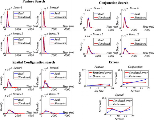
The data used in this paper was collected as part of Lin et al.’s (2015) experiments. Details of the design can be found in Lin et al. (2015). The search displays were arranged in a circular layout (see Figure 1) in which items can be placed in 25 locations. The display size was 3, 6, 12 or 18 items. Each condition comprised 100 trials. Three different search experiments were conducted: feature search, conjunction search, spatial configuration search. In the feature search task, the target was a dark square while the distractors were grey squares. In the conjunction search, participants looked for a vertical dark bar amongst two types of distractors, vertical grey bars and horizontal dark bars. The spatial configuration task used two items, digit 2 (target) and digit 5 (distractor). Each search task was completed by 20 participants; one participant was removed from feature and conjunction search tasks due to high error rates. Figure 2 shows the resulting search functions for the present condition. In addition, Lin et al. (2015) found that for feature search and conjunction search the RT distribution’s skewness increased with increasing display size. For spatial configuration search the relationship between skewness and display size was more complex. The skewness first increased over the smaller display sizes (3, 6, 12) but then decreased from 12 to 18.

Figure 1. Schematic representation of the tasks. From left to right: feature search, conjunction search, spatial configuration search.

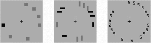
Figure 2. Search functions of the three tasks (feature search, conjunction search, spatial configuration search) used in this study. The error bars indicate the standard error.

The results indicate that the data provides a good basis for testing the models on a range of search task difficulties similar to Wolfe et al.’s (2010) data. However, there is an interesting difference between their data and our data. In our study, participants made roughly twice as many as errors as in their experiments. This difference can be explained because in Wolfe et al.’s (2010) experiments, participants completed all three tasks with 500 trials in each condition. In our study, participants completed only 100 trials per condition and not all tasks. Thus, in Wolfe et al.’s (2010) study participants were highly practiced compared to our study. When we re-analysed Wolfe et al.’s (2010) data and included only the first 100 trials of each condition the error rates were similar to our error rate. Hence our dataset poses the interesting challenge to CGS whether CGS will also be able to model less practiced participants.

Computational models

SAIM’s winner-take-all model

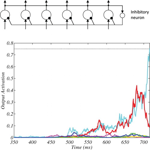
The biased competition model is based on SAIM’s WTA mechanism (Heinke & Backhaus, 2011; Heinke & Humphreys, 2003; Zhao, Humphreys, & Heinke, 2012). This WTA mechanism uses a single layer of “neurons” which are connected by a lateral inhibition (see Figure 3(a)). If the correct parameters are chosen, the neuron with the highest input is activated while all other neurons are shut down (see Figure 3(b) for an exemplar simulation result). In other words, all neurons compete with each other and the neuron with the largest input wins the competition. The mathematical description of the model as follows:$\text{d}{x}_i=-\frac{\text{d}t}{\tau }{x}_i+\frac{\text{d}t}{\tau }\left(w\left(\sum _{j=1}^n{y}_j\right)+I_i\right)+\sqrt{\frac{\text{d}t}{\tau }}{\xi }_i;$ $y_j=f\left(x_j\right)=\frac{1}{1+e^{-m(x_j-s)}};\xi =N(0,\sigma );$

Figure 3. The graph at the top shows SAIM-WTA’s architecture. All nodes compete via global inhibitory neuron. The time course at the bottom shows an example of SAIM-WTA’s output activation. The line colours correspond to the network’s nodes. The dotted line indicates the threshold for this particular simulation. The simulation result came from the spatial configuration search with six search items and the parameters from the 8th participant (see Appendix I).

where f(x) is a sigmoid function with parameters slope (m) and intercept (s), $\tau$ is the accumulation rate of input activation and w is the strength of the lateral inhibition, $\xi$ is Gaussian noise with the variance $\left(\sigma \right)$, $I_i$ is the input to the ith neuron, $y_i$ is the output activation of ith neuron, $x_i$ is the internal activation of the ith neuron. These equations are based on a mathematical description of neurophysiological processes using a spiking-rate neuron model. The Gaussian noise takes into account the randomness of neural processes. The sigmoid function models the non-linear relationship between cell activation and output spiking rate. The differential equation models the leaky accumulation behaviour of synapses. The summation term realizes the lateral inhibition within the layer (inhibitory neuron).

To adapt the model to modelling visual search data, we made several simple assumptions. Each “neuron” is assumed to correspond to an item location in the search display. If a location is empty the input is set to zero. The neuron for the target location is set to one while the distractor neurons are set to a saliency value. To model the reaction time, we introduced a decision boundary and computed the time it takes for a neuron to pass this threshold. If it is a distractor neuron the response is recorded as “target absent”; if it is a target neuron the response is “target present”.

It is worth noting that SAIM-WTA is similar to the Leaky Competing Accumulation (LCA) model (Usher & McClelland, 2001). However, to the best of our knowledge, LCA has never been applied to visual search. Moreover and similar to LCA, SAIM-WTA stands in the tradition of the Parallel Distributed Processing (PDP) framework (Rumelhart & McCleland, 1986) in that it draws on principles of neural information processing in order to understand phenomena at the behavioural level (see Mavritsaki, Heinke, Allen, Deco, & Humphreys, 2011, for a discussion of linking the neural level with the behavioural level through means of computational models).

In addition, some mechanisms and conceptualizations are also similar to stochastic drift diffusion models (Busemeyer & Diederich, 2010; Ratcliff, 1978). These models assume that perceptual decision making is based on an accumulation of perceptual information. Once this accumulation has reached a certain level (i.e., threshold) a decision is made (i.e., a response is generated). The time it takes for the accumulation to reach the threshold is interpreted as reaction time. SAIM-WTA can be framed in terms of these drift diffusion models in that SAIM-WTA’s model accumulates information about the search items (i.e., identifies them) and once this information has reached a certain level the model/participant initiates a corresponding response. However, and different from drift diffusion models, the accumulators interfere with each other.

SAIM-WTA has seven free parameters. In explorations of the parameter space prior to work presented here, we found several regions where it was possible to achieve a similar quality of fit. Subsequently, we focused on a region where it was possible to reduce the number of free parameters to the smallest possible number (i.e., three) while still obtaining the best fits for all participants (see Appendix I for the values of the fixed parameters). In addition, the remaining free parameters (accumulation rate, decision boundary, distractor saliency) allowed us to ask interesting theoretical questions about the factors which influence visual search performance. Given the biased-competition theory’s assumptions, we expect that the distractor saliency (target–distractor similarity) increases with task difficulty, but it is not clear if the distractor saliency is sufficient to explain the differences between the tasks or is there also a difference in terms of the difficulty of identifying items (as expressed by accumulation rate)? In fact, computational models such as SAIM (and CGS) suggest the involvement of a separate object identification stage.

Competitive Guided Search (CGS)

Moran et al.’s (2013) CGS implements a serial search based on Wolfe’s (2007) two stage architecture. The guidance through the saliency map is implemented through a probabilistic selection where target item has the probability to be selected:$p_{\mathrm{target}}=\frac{w_{\mathrm{target}}}{n-1+w_{\mathrm{target}}}.$and the distractor items:$p_{\mathrm{distractor}}=\frac{n-1}{n-1+w_{\mathrm{target}}}.$ $w_{\mathrm{target}}$ is the saliency of the target relative to the distractor. If the target saliency is smaller than one there is no guidance; n is the number of items currently available for selection and is decremented after each search step. Hence, CGS assumes that once an item is identified it is not revisited again. Prior to each search step, CGS decides whether to continue with the search, or to quit the search and decide that the target is absent. The probability to quit is calculated in the following way:$p_{\mathrm{quit}}=\frac{w_{\mathrm{quit}}}{w_{\mathrm{quit}}+n-1+w_{\mathrm{target}}}$Again, n is decremented after each search. Hence, the probability to quit increases with each search step. This effect is increased further by modifying $w_{\mathrm{quit}}$ at each search step:$w_{\mathrm{quit},\mathrm{new}}=w_{\mathrm{quit},\mathrm{old}}+\mathrm{\Delta }{w}_{\mathrm{quit}}$Note that the value of $w_{\mathrm{quit}}$ is zero at the beginning of the search.

At each search step, CGS assumes that an item is identified as to whether it is a target or a distractor. This identification process is modelled as a drift diffusion process which is also used to describe the behaviour of SAIM-WTA’s nodes. However, instead of simulating the drift diffusion process Moran et al. (2013) used the Wald distribution to represent the distribution of the identification time (i.e., passing of threshold):$p_{\mathrm{wald}}(t|\alpha ,v,\sigma )=\sqrt{\frac{{\left(\alpha /\sigma \right)}^2}{2\pi x{t}^3}}{e}^{{\displaystyle \frac{-{\left(\alpha /\sigma \right)}^2{(t-(\alpha /v\left)\right)}^2}{2{\left(\alpha /v\right)}^{2}t}}}$with the three parameters identification drift rate ($\upsilon$), identification threshold ($\theta$) and noise level ($\sigma$). The noise level was fixed at 0.1 throughout the studies. The total reaction time is the sum of all identification times from all search steps. Moran et al. (2013) also chose this distribution as Palmer et al. (2011) found this distribution to be the best to describe Wolfe et al.’s (2010) data.

Note that mathematically the probability distribution of the sum of independent random variables can be determined by convolving the probability distributions of the individual random variables. Hence, CGS’s total reaction time can be described as multiple convolutions of a Wald distribution where the number of convolutions depends on the number of search steps. One consequence of this convolution is that CGS’s RT distribution is more skewed the more search steps take place. Hence, CGS should produce an increase in skewness with increasing display size (depending on the search task). This relationship should enable CGS to model RT distributions from visual search tasks.

CGS also assumes that at the response execution stage an erroneous response can occur due to a motor error with a certain probability ($m$). Since the identification stage is assumed to be perfect, misses of targets can only occur through motor errors. It is also worth noting that motor errors can “correct” misses as it is possible that search terminates without finding the target but due to an error the model still reports “target present”. Finally, a residual time accounts for the duration of processes which are outside the actual search process such as encoding of items, post-decisional processes, response planning and execution. The residual time is assumed to be distributed as a shifted exponential distribution with non-decision shift time ($T_{\min }$) and non-decision drift time ($\gamma$) as parameters.

Discussion

Apart from implementing two different types of searches, the models relate differently to the neural substrate. SAIM-WTA aims to be “biologically-plausible” while CGC is less rooted in neural processes, even though the identification stage has a similar link (drift diffusion model) to neural processes as SAIM-WTA. Both models assume item identification plays a critical role in visual search.

The selection process from the saliency map is seen by CGS’s authors as an approximation of a competition process (hence competitive Guided Search). However, the approximation does not involve interference between items as SAIM-WTA implements. Hence, the selection process is probably better understood as a randomized selection process which is modulated by item saliency.

However, for the purpose of this paper these differences and commonalities are less important. More important is the fact that SAIM-WTA has fewer free parameters than CGS. SAIM-WTA absorbs CGS’s stages (identification stage, encoding stage, etc.) into the competition process. Hence, a numerical comparison between the models can look at whether this more parsimonious model is more successful than a more complex model.

Method

Both models were fitted to each participant separately. The resulting quality of fit and parameter settings were averaged in order to represent the population level.

The best fitting parameter settings were determined using the maximum likelihood principle (MLP). MLP allows us to base model fit on RT distributions. To employ MLP, traditionally it is necessary for models to possess an analytic probability density function (pdf). However, models such as SAIM-WTA or GCS don’t possess such pdfs. Recent developments in model fitting, often termed approximated Bayesian computation (ABC) or “likelihood-free methods” (see Beaumont, 2010, for a review) solve this issue by approximating the model’s pdfs. We utilized a likelihood-free method based on a KDE-approach which estimates the model’s pdf for a given parameter setting using Monte Carlo sampling (see Turner & Sederberg, 2014). In the following section, we will introduce the KDE-method we used here. After that, we will discuss the method we used to find the best-fitting parameters. Since the representation of RT distributions and the method for parameter search are different from Moran et al.’s (2013) methods, we include a brief explanation of why we have chosen different methods. At the end of this section we will explain how we removed outlier parameter settings.

Model’s pdf

In this paper, we utilize a novel KDE method, on-line KDE (oKDE; Kristan et al., 2011). The method was chosen as it is ideal for approximating RT distributions even with 100 trials (see Appendix III for a demonstration). Originally, the KDE method was proposed by Silverman (1986). A KDE is based on a sum of distribution kernels (either Gaussian or Epanechnikov distributions). The number of kernels is equal to the number of data points. The mean of each kernel is the value of the corresponding data point and the variance for all kernels (bandwidth) is estimated from the data’s variance (see Van Zandt, 2000, for details). The oKDE method is more flexible in terms of number of kernels and their variance. In fact, oKDE optimizes the number of kernels and their widths (see Figure 4). Hence, oKDE leads to a more efficient and more adaptable KDE than the standard KDE method (Kristan et al., 2011, for detailed discussion). Initially, the oKDE method assumes a kernel for each data point (similar to the traditional KDE-approach) and determines the smallest bandwidth for this initial KDE using an optimality criterion. Subsequently, oKDE clusters these kernels to construct kernels with larger bandwidths (see Kristan et al., 2011, for details).

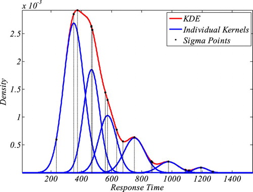
Figure 4. An illustrative example of how oKDE decomposes a distribution in several kernels with varying variance. The example also shows the location of the sigma points in this KDE which were relevant for the evaluation of the KDE (see Appendix III for details).

Parameter search

To find the optimal parameters, we utilized a particular version of a differential evolution (DE) algorithm (Storn & Price, 1997; ter Braak, 2006). DE algorithms aim to implement a near global search through parameter space by utilizing populations of parameter settings (rather than a single parameter setting) as the starting point for the search (see Comparison with Moran et al.’s [2013] method for more details). The particular version we used was the probabilistic Markov chain Monte Carlo (DE-MCMC) extension by Turner, Sederberg, Brown, and Steyvers (2013). A main advantage of the differential algorithms is their natural ability to deal with correlations between parameters. For instance, accumulation rate and decision boundary are correlated as an increase in decision boundary leads to an increase in reaction times in a similar way as a decrease in accumulation rate leads to an increase in reaction times.

Likelihood function

The fit of the model with the data was evaluated with the likelihood principle using a pdf for mixed data (Turner & Sederberg, 2014):$L\left(S|\theta \right)=\prod _{j=1}^2\prod _{i=1}^{X=s_j}P\left(s_j\right)M_j\left(x_i|\theta \right)$where P(s₁) is the probability of correct response and P(s₂) is the probability of incorrect response. M_j(x_i|θ) denotes the model’s pdf for any observation x_i, the parameters θ and response type (j). As stated earlier, here the model’s pdf is represented by a KDE. However, this likelihood function is not fully suitable for our modelling approach, as we don’t consider the reaction times for incorrect responses. Therefore, Turner and Sederberg’s (2014) equation turns into:$L(X_c,X_i|\theta )=(1-P(X_c){)}^{n_i}\prod _{j=1}^{n_c}P(X_c\left)M\right(x_j\left|\theta \right)$where n_i indicates the number of incorrect responses and n_c is the number of correct responses. P(X_c) is the probability of correct responses in the model.

In addition, we improved the robustness of estimating the likelihood function at unlikely data points by introducing a dataset-defined threshold for the model’s pdf. Note that thresholding very small pdf values is common practice to avoid numerical issues (i.e., underflow) in the calculation of likelihood values. In standard applications, this practice does not lead to large problems as the model’s pdf is typically similar to the data (e.g., Weibull distribution as model of RT distributions) and so small pdf values relate to rare occurrence of data points. However, in our modelling enterprise the model’s pdf needs to be created via Monte Carlo sampling which sometimes leads to a misrepresentation of the model’s pdf particularly for unlikely simulation outcomes (i.e., unlikely data points). In other words, the KDE constructed from such a sampling error assigns small probabilities to these data points; even smaller than implied by their presence in the dataset. Other sampling runs with similar parameter settings may assign reasonable probabilities to these data points. Such variations in sampling can lead to large problems in finding optimal parameters during the parameter search. To stabilize this (i.e., improving the robustness of estimating the likelihood function), we introduced this data-defined threshold. In order to determine this threshold, we fitted a KDE to the dataset. As stated earlier, initially the oKDE method assumes a kernel for each data point (similar to the traditional KDE approach) and determines the smallest bandwidth for this initial KDE using optimality criteria. This bandwidth defines a lower bound for a probability of a data point. Hence, any pdf constructed for a model (KDE) should produce at least this probability for each data point. Therefore, this bandwidth forms a reasonable threshold for the model’s pdf (KDE). In other words, if the model is correct, a failure to produce reasonable probabilities for unlikely data points has to be due to the sampling error and thresholding the model’s KDE in this situation corrects this error. However, sampling error is not the only reason for failing to produce reasonable probabilities. Suboptimal parameter settings can lead to model pdfs which are very different from the data’s pdf. In this situation, the threshold introduces a bias towards a better evaluation of the model. To lower this bias, we reduced the data-driven threshold by 50%:$L\left(X|\theta \right)=\prod _{i=1}^n\text{max}\left(M\right(x_i|\theta ),N(0,h\left)/2\right)$where h is the smallest bandwidth.

Comparison with Moran et al.’s (2013) methods

To fit parameters, Moran et al. (2013) used the popular algorithm by Nelder and Mead (1965) which is implemented in MatLab’s fminsearch. This method is very sensitive to the choice of the starting point of the parameter search. Our DE-MCMC method reduces this problem by using a population of starting points.¹ Moreover, to estimate the RT distributions Moran et al. (2013) employed the commonly used Quantile Maximal Probability (QMP) method by Heathcote, Brown, and Mewhort (2002). However, Turner and Sederberg (2014) showed that this method can lead to misleading results.

Thus, given the differences between our approach and Moran et al. (2013), attempting to replicate Moran et al.’s (2013) parameter settings is unlikely to be successful. However, to demonstrate that our approach is more reliable than Moran et al.’s (2013) approach, we fitted CGS to Wolfe et al.’s (2013) data twice, using different starting points. First, Moran et al.’s (2013) parameter settings from the individual participants were used as starting points for the parameter search. Even though these starting points are unlikely to be the best fits given the differences in methods, they should at least be close to very good solutions which DE-MCMC would be able to find. Second, we used our parameter settings established by fitting Lin et al.’s (2015) data. Interestingly, the quality of fit for Moran et al.’s (2013) parameter settings as starting points was not as good as for our parameter settings as starting points. Hence, we conclude that our parameter settings generalize better across different datasets while Moran et al.’s (2013) settings seem very specific to their chosen starting point of the search.

Removal of outlier parameter settings

It turned out that some participants’ parameter settings were extreme. We therefore applied an outlier elimination method, the median absolute deviation (MAD; Leys, Ley, Klein, Bernard, & Licata, 2013), to each parameter in each task. As criterion for an outlier we used five standard deviations. A participant was identified as outlier if at least one parameter value was considered to be an outlier. This participant was removed from the further analysis.

Results and discussion: SAIM-WTA

We fitted SAIM-WTA with three free parameters (distractor saliency, decision boundary, accumulation rate) to Lin et al.’s (2015) 58 datasets from three visual search experiments (feature search, conjunction search, spatial configuration search). Hence, we obtained 58 parameter settings (see Appendix II for values), 19 parameter settings (participants) for feature search, 19 settings (participants) for conjunction search and 20 settings (parameters) for spatial configuration. Eyeballing the parameter settings, we noticed that there were a few settings which could be considered as outliers. Our outlier detection procedure led to the removal of two participants from feature search, three settings from conjunction search and no participant from spatial configuration search.

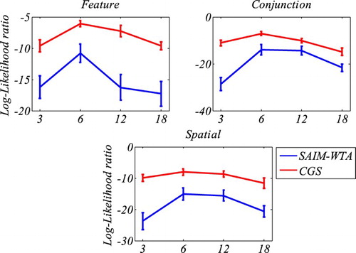
To assess the overall fit for each participant we calculated the log likelihood ratios (log likelihood value from the model divided by the log likelihood value of the KDE’s dataset; see Figure 5 for the results). We compared ratios from the different tasks with the Wilcoxon rank-sum test and found a significant decline of ratios between feature search and conjunction search ($z=2.36;p=.018$); and feature search and spatial configuration ($z=2.85;p=.004$). There was no significant difference between conjunction search and spatial configuration search ($z=0.14;p=.886$). 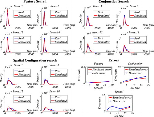To illustrate the quality of fit (likelihood ratio), Figure 6 shows the outcome from three participants. Note that the choice of these participants was made randomly by MatLab to avoid an author bias. The likelihood ratio was −46.32 for feature search, −61.10 for conjunction search and −71.98 for spatial configuration search. The graphs indicate that SAIM-WTA was able to produce an increased skewness with increased display size. This increase broadly matched the increase of skewness in the data, but not to the same degree. The failure to match skewness is particularly pertinent in spatial configuration search for display size 18. This effect is illustrated in Figure 10 where the likelihood ratio declined with increasing display size. Nevertheless, it is important to note that the only source of this effect is the increase of number of distractors in the input of the model since all parameters are kept constant. In other words, the competition between items due to lateral inhibition is able to explain the skewness found in the visual search.

Figure 5. Results of fitting SAIM-WTA. The top-left graph shows the mean log-likelihood ratios (quality of fit) for the different tasks. The remaining graphs show the mean parameters. The error bars indicate the standard error.

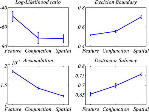
Figure 6. SAIM-WTA. KDE-based illustration of RT distributions and response errors. Note that these graphs show the RT distributions for three participants.

Figure 5 shows how the three free parameters (distractor saliency, decision boundary, accumulation rate) changed across the three tasks. The parameters were entered into a Wilcoxon rank-sum test. For accumulation rate, there was significant difference between feature search and conjunction search (z = 4.845, p < .001) as well as between conjunction search and spatial configuration search (z = 4.056, p < .001). For distractor saliency, the difference between feature search and conjunction search was significant (z = −2.684, p = .007) and so was the comparison between conjunction search and spatial configuration (z = −3.659, p < .001). For decision boundary, both comparisons were also significant (z = −3.368, p < .001; z = −4.619, p < .001). Hence all comparisons were significant. As expected, the distractor saliency increased with increasing task difficulty. However and interestingly, the other two parameters were also related to task difficulty. Accumulation rate decreased with increasing task difficulty, i.e., framed in terms of drift diffusion models, discussed earlier, the accumulation of perceptual information about items was more and more difficult. Finally, it is worth noting that the level of decision boundary increased with task difficulty. A closer inspection of this finding showed that it is a by-product of the increase of competition leading to higher activations of distractors requiring higher decision boundaries to avoid response errors.

On the whole, SAIM-WTA exhibited a reasonable fit with three search tasks. In particular, it was able to model the increasing skewness with increase in display size. However, the quality of fit decreased with task difficulty. In particular, SAIM-WTA was not able to match the increase in skewness with increased display size.

The three free parameters (distractor saliency, accumulation rate, decision boundary) were different for the three tasks. Distractor saliency increased across tasks as predicted by all major theories on visual search. Importantly, SAIM-WTA identifies distractor saliency as an important source for the increase in skewness across display sizes. The results also identify an increase of accumulation rate with task difficulty. As discussed in the introduction of WTA-SAIM, accumulation rate can be linked with object identification. In other words, SAIM-WTA indicates that not only does selection of target get more difficult across the three tasks, but also object identification gets harder. This is consistent with other theories on visual search, such as biased-competition theory, and with computational models such Moran et al.’s model and SAIM. However, both models consider object identification as a separate processing stage. Moreover, this offers an interesting explanation for findings that responses in pop-out searches can be speeded up even further by additional manipulations such as priming (Maljkovic & Nakayama, 2000; Woodgate et al., 2015). SAIM-WTA suggests that the speed-ups are due to improved target identification. Fitting SAIM-WTA to data from priming experiments should support this prediction.

Finally, the increase of the decision boundary makes an interesting prediction for an application of the Speed–Accuracy Tradeoff (SAT) procedure in visual search experiments. In a SAT procedure, participants’ response time is controlled by requiring them to respond within a set time window (Wickelgren, 1977; Zhao et al., 2011). For early time windows where participants sacrifice accuracy for speeded responses, SAIM-WTA should detect lower decision boundaries, but distractor saliency and accumulation rate remain unchanged.

Results and discussion: Competitive Guided Search

We fitted CGS with seven free parameters (target saliency, identification drift, identification threshold, quit weight increment, non-decision time shift, non-decision time drift, motor error) to Lin et al.’s (2015) 58 datasets from three visual search experiments, feature search, conjunction search and spatial configuration search. Thus we obtained 58 parameter settings (see Appendix II for values), 19 parameter settings (participants) for feature search, 19 settings (participants) for conjunction search and 20 settings (parameters) for spatial configuration. Our outlier removal procedure detected no outlier for feature search, two outliers for conjunction search and two outliers for spatial configuration. It is also worth noting that the parameter search revealed that there are good fits for conjunction search and feature search where the saliency values are implausibly high. This is not very surprising as fast target searches can be executed with arbitrarily high saliency value. To solve this problem, we first fitted spatial configuration and used these resulting parameter values as starting point for fitting the other searches. This way the best fits produced saliency values which were relatively small (see note 1).

To assess the overall fit for each participant, we calculated the log likelihood ratios, i.e., log likelihood value from the model divided by the log likelihood value of the KDE’s dataset. We compared ratios from the different tasks with the Wilcoxon rank-sum test and a significant difference was found between feature search and conjunction search ($z=2.92;p=.004$); and feature search and spatial configuration search ($z=3.11;p=.002$). And there was no significant relation between conjunction search and spatial configuration search ($z=0.25;p=.81$). Figure 7 shows that the quality of fit declined with task difficulty. To illustrate the quality of fit, Figure 8 shows the outcome from three participants. Note that the choice of these participants was made randomly by MatLab to avoid an author bias. The likelihood ratio was –18.44 for feature search; −38.82 for conjunction search and −44.10 for spatial configuration search. The graphs illustrate that CGS’s distributions nicely overlap with the RT distributions from the respective tasks. Hence, we were able to qualitatively replicate Moran et al.’s (2013) results.

Figure 7. Results of fitting CGS. The top-left graph shows the mean log-likelihood ratios (quality of fit) for the different tasks. The remaining graphs show the means of CGS’s seven parameters for the three tasks (Feature Search = FS; Conjunction Search = CS; Spatial configuration search = SC). Note, for the purpose of a better illustration the target saliency parameter was scaled logarithmically. The results replicate Moran et al.’s (2013) findings. The error bars indicate the standard error.

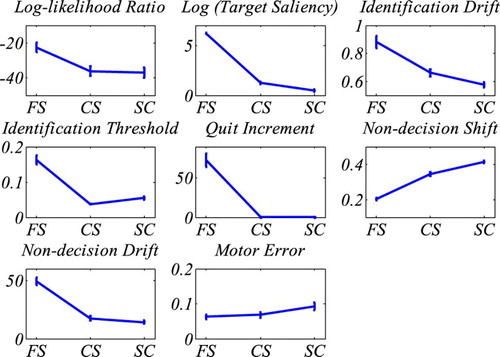
Figure 8. CGS. KDE-based illustration of RT distributions and response errors. Note that these graphs show the RT distributions for three participants.

Interestingly, we were also able to replicate the qualitative relationship of parameter values with the search tasks (see Figure 7 and Moran et al. (2013); Appendix C). The parameters accounting for encoding and post-decisional process showed longer delay (non-decision shift) and more variance (non-decision drift) with increasing task difficulty. Motor error increased with task difficulty. The identification drift showed slower accumulation rate with increasing task difficulty. The identification threshold decreased with task difficulty (albeit counterintuitively). The likelihood to stop scanning the search display (w_quit) increased less the more difficult the task was. Finally, the guidance (target saliency) was smaller the harder the task was. Interestingly, and similar to Moran et al.’s (2013) findings, there was still residual guidance in the spatial configuration search task. In fact, there was no significant difference between our guidance parameters and Moran et al.’s (2013) parameters (see Table II.1 for a comparison using Wilcoxon rank-sum test). These findings question Moran et al.’s (2013) explanation for their result. They stipulated that guidance may be possible due to the fact that participants were highly practiced in Wolfe et al.’s (2010) dataset. However, in Lin et al.'s (2015) experiment the participants were not practiced and CGS still suggests that there is guidance involved. Since our numerical methods were different from Moran et al.'s (2013) methods, as discussed earlier, we also fitted CGS to Wolfe et al.’s (2010) dataset using our numerical methods. Again, we found no significant difference between the saliency values for Wolfe et al.'s (2010) dataset and for Lin et al.’s (2015) dataset. Since practice effects go beyond the topic of the present paper we did not follow this up any further.

Comparison of SAIM-WTA and CGS

Figure 9 compares SAIM-WTA and CGS in terms of log-likelihood ratio. Overall, it demonstrates that CGS explained the visual search data better than SAIM-WTA. The only exception is conjunction search where CGS and SAIM-WTA showed similar results. Figure 9 also breaks down to the results in terms of how well the two models explained the data for the different display sizes. Figure 9 gives us an insight into why SAIM-WTA is worse than CGS and highlights a problem with both models. The graphs show that, irrespective of display size, SAIM-WTA performed worse than CGS. Hence, SAIM-WTA failed to replicate the RT distributions with the same precision as CGS. However, both models showed their best fit with display size 6 and then a decline in quality for larger and smaller display sizes. In other words, their ability to explain the influence of display size and their effect on RT distributions does not generalize to all display sizes equally well. Hence, both models need to be improved in this respect.

Figure 9. Comparison of mean log likelihood ratios from SAIM-WTA and CGS for the three tasks (feature search, conjunction search, spatial configuration). The graphs indicate the contributions from the different display size to the overall log likelihood ratios. The error bars indicate the standard error without within-participant variance (Cousineau, 2005). The graphs demonstrate that CGS was better at explaining the data than SAIM-WTA. However, they also show that the performance of both models is best at display size 6 and worse at all other display sizes (see main text for more discussion).

The log-likelihood ratio does not take into account the complexity of models. This difference of complexity (as measured in terms of number of parameters) is particularly marked between CGS and SAIM-WTA. Normally, model complexity is included in a model comparison by using the Akaike information criterion (AIC) and/or the Bayesian information criterion (BIC). Both criteria penalize the quality of fit by the number of parameters needed to achieve this quality, whereby BIC penalizes the quality more than AIC. Also note that the smaller the AIC/BIC scores, the better the model. Figure 10 shows the results for AIC and BIC. Since the results for the two models are quite close we also entered the AIC values into a Wilcoxon sign-rank test (see Table 1). The results show that, apart from conjunction search, CGS performs better than SAIM-WTA. However, the difference in the range of 2 and 3.82 for AIC and the range of 2.29 and 3.58 for BIC is not very large.

Figure 10. Comparison of BIC scores and AIC scores from SAIM-WTA and CGS for the three tasks (feature search, conjunction search, spatial configuration search). The error bars indicate the standard error without within-participant variance (Cousineau, 2005). BIC and AIC penalize the quality with the model complexity as measured with the number of parameters. The graphs indicate that CGS performed better than SAIM-WTA despite SAIM-WTA being the simpler model.

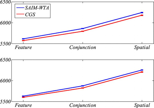
Table 1. Comparison of BIC scores and AIC scores from SAIM-WTA and CGS for the three tasks (feature search, conjunction search, spatial configuration search) using Wilcoxon sign-rank test.

z-value, p-value	AIC	BIC
Feature	3.62, <0.001	2.29, 0.022
Conjunction	3.82, <0.001	3.58, <0.001
Spatial	3.55, <0.001	2.95, 0.003

Note: All comparisons were significant. For all comparisons CGS showed better results than SAIM-WTA.

General discussion

This paper aimed to contribute to the long-standing dispute on parallel versus serial search. In order to do so, we numerically fitted two computational models to RT distributions from three visual search experiments (feature search, conjunction search, spatial configuration search). The two computational models, CGS (Moran et al., 2013) and SAIM-WTA (Heinke & Backhaus, 2011) implement a serial and parallel search respectively. The comparison of the two models’ success to explain the RT distributions is expected to advance our understanding of visual search in humans. It also allows us to demonstrate how RT distributions can contribute to this enterprise.

In order to fit the models to the RT distributions, we employed a novel KDE which allowed us to base evaluations of the fits on the maximal likelihood criteria. We used the differential evolution Markov chain Monte Carlo (DE-MCMC) method to find the best fit. The paper demonstrated that these methods can successfully fit computational models to RT distributions from the visual experiments. We also showed that the KDE is an excellent method to represent RT distributions.

The results with SAIM-WTA showed for the first time that a biased-competition model is able to reproduce RT distributions from visual experiments, in particular the increased skewness linked with increased display size. The results with CGS demonstrated that the model generalized well to new data. This success also highlights the validity of our new model fitting method. However, a direct comparison between SAIM-WTA and CGS revealed that CGS fits better to RT distributions than SAIM-WTA. This is the case even if the evaluation takes into account that CGS is a more complex model than SAIM-WTA. In other words, GCS’s Wald distribution modelling the item identification at search step constitutes a better description of search behaviour than the RT distribution generated by SAIM-WTA’s competition process. The addition of identification times by the way of serial search scans (mathematically the multiple convolutions of Wald distributions) represents fairly well the increase of mean RTs and their increased skewness. However, it is notable that both models don’t generalize well across different display sizes as the quality of fit for both models decreases with increasing display size. It is also worth pointing out that we fitted CGS and SAIM-WTA to Wolfe et al.’s (2010) data. As this data set does not contain as many participants as Lin et al.’s (2015) dataset, the results were not as statistically conclusive as the ones presented here. Also, some parameter settings were statistically different than ones presented here. These differences are certainly due to methodological differences, some of which we discussed in the section about Lin et al.’s (2015) dataset. Since these differences go beyond the scope of this paper we have not included reports of those results. However and importantly, the overall findings presented here, that CGS is slightly better than SAIM-WTA in explaining visual search experiments, was replicated. In other words, we can be quite confident that our results are valid for these three visual experiments irrespective of the methodological details, such as display geometry and practice effects.

What are the lessons from this model comparison for SAIM-WTA and CGS? It shows that SAIM-WTA produced excellent fits, but CGS produced slightly better fits. This is probably due to the fact that Moran et al. (2013) chose to model the identification of each item with a Wald distribution which in turn was motivated by Palmer et al.’s (2011) finding that the Wald distribution is the best distribution compared to other skewed distributions such as ex-Gaus or Weibull. Hence, it will be important for the progress of SAIM-WTA to find a way to produce more Wald-like distributions. A possible solution is to add an identification stage. Such an identification stage would lead to more skewed RT distributions, possibly enabling SAIM-WTA to produce better fits for larger display sizes. Finally, it is also worth noting that SAIM-WTA was not specifically designed to model visual search and instead aimed to capture a broad range of experimental evidence typically associated with visual selective attention. Hence, matching CGS’s performance or even surpassing it was always a difficult goal to achieve.

In addition, SAIM-WTA (and CGS: see below) will have to improve on how the display size influences its reaction times. It is interesting to note that on the whole the quality of fit decreases increased with increasing display size. This may point to a possible cause of this problem. Of course, with increased display density the spatial proximity between items increases. Hence, it is conceivable that perceptual grouping (Wertheimer, 1923) plays an increasing role in higher display sizes. Hence, a sensible extension of SAIM-WTA may be to integrate a grouping mechanism into the competition process. For instance, at present the inhibitory connections are homogenous independent of an item’s position. An extension of SAIM-WTA may modulate these weights depending on the distance between items. A corollary of this line of argument is that perceptual similarities between items may also play a role in visual search. Of course, this is not a new idea and there is already evidence for this, in particular from the seminal paper by Duncan and Humphreys (1989) (see also Müller-Plath & Elsner, 2007, for a systematic variation of spatial proximity and item similarity). In any case, this extension of SAIM-WTA will have to be tested with a series of studies manipulating grouping in visual search possibly along the lines of Müller-Plath and Elsner’s (2007) work.

Obviously, an integration of a grouping mechanism into CGS’s saliency map along similar lines is also possible, and this modification may lead to the desired effect of improving the fit with higher display sizes. However, such a modification would not improve CGS’s serial process as such. Instead, a simple modification of CGS consistent with its serial tenet could be to let the parameters of the identification stage depend on at which point in the serial search scan the items are identified. This additional mechanism could slow down identification or make RT distributions more skewed the later an item is selected, possibly improving CGS’s performance for larger display sizes. This modification can be seen as some sort of inhibition effect on the identification stage (object-based inhibition, Egly, Driver, & Rafal, 1994; Heinke & Humphreys, 2003, Study 5). However, it is highly questionable whether this new mechanism can successfully explain the potential influence of perceptual grouping as discussed earlier since it does not consider spatial proximity of items or item similarity. On a more general note, it is worth pointing out that it is difficult to imagine how CGS’s slow serial identification process can model perceptual grouping in a plausible way (serially scanning through some items and making them a group if they are the same would be far too slow). Hence, these difficulties of CGS with perceptual grouping suggest that the series of visual experiments manipulating grouping, as suggested earlier, can produce data which allow for a stronger comparison between serial and parallel models where even the parallel approach may win the competition.

In conclusion, we have demonstrated that it is possible to constrain computational models of visual search with RT distributions. We were also able to replicate findings from a serial model of visual search (CGS; Moran et al., 2013). In addition, we successfully fitted a parallel (biased competition) model of visual search (SAIM-WTA; Heinke & Backhaus, 2011) to RT distributions for the first time. When the two models were compared, the serial model was able to explain better RT distributions from three visual search tasks. However, both models exhibited deficits in how they dealt with different display size. From the discussion of possible mechanisms to iron out this problem, we inferred that a series of visual experiments manipulating perceptual grouping should lead to a stronger test for the models.

Acknowledgements

We would like to thank the three anonymous reviewers for their helpful and constructive comments.

Disclosure statement

No potential conflict of interest was reported by the authors.

ORCID

D. Heinke http://orcid.org/0000-0003-3632-7569

Additional information

Funding

This work was supported by Engineering and Physical Sciences Research Council DTA to VN [grant number: EP/K502984/1].

Notes

1. This sensitivity to the starting point of a search is because complex models like the ones used here have many local solutions. These local solutions are the best solutions in particular areas of the parameter space, but it is not clear whether a particular local solution is the overall best solution (global solution). Most, if not all, methods for parameter search find (get trapped in) local solutions and cannot guarantee that this is the global solution. Amongst other factors the starting point of the search is critical for which local solution is found. Broadly speaking, search algorithms tend to find local solutions near the starting point.

Appendices

Appendix I

SAIM-WTA

Table

Constant parameters	Noise	Sigmoid slope	Sigmoid shift	Inhibitory weight
	0.1	50	0.5	−1

The gamma-parameter in DE-MCMC was set to $2.38/\sqrt{2d}$ where d refers to the number of free parameters. A constant random noise was set to all parameter proposals of 0.001.

Table

Feature Search Participant	Decision Boundary	Accumulation	Distractor Saliency	Outlier
1	0.5128	0.0019	0.6642	No
2	0.5214	0.0018	0.6537	No
3	0.5020	0.0017	0.6196	No
4	0.5067	0.0018	0.6381	No
5	0.5276	0.0016	0.0635	Yes
6	0.5011	0.0018	0.6672	No
7	0.5035	0.0019	0.6849	No
8	0.5079	0.0019	0.7145	No
9	0.5190	0.0020	0.6636	No
10	0.5297	0.0020	0.6413	No
11	0.5249	0.0016	0.5686	No
12	0.5221	0.0018	0.6756	No
13	0.5068	0.0020	0.6695	No
14	0.5184	0.0019	0.2815	Yes
15	0.5503	0.0018	0.6467	No
16	0.5047	0.0020	0.6612	No
17	0.5412	0.0017	0.6884	No
18	0.5058	0.0021	0.5642	No
19	0.5075	0.0019	0.6968	No

Table

Conjunction Search Participant	Decision Boundary	Accumulation rate	Distractor Saliency	Outlier
1	0.5762	0.0015	0.7192	No
2	0.5709	0.0017	0.7067	No
3	0.5056	0.0015	0.6181	No
4	0.5503	0.0014	0.7780	No
5	0.7373	0.0012	0.6394	Yes
6	0.5228	0.0013	0.6968	No
7	0.5226	0.0014	0.8034	No
8	0.5927	0.0013	0.7208	No
9	0.5177	0.0015	0.6557	No
10	0.8288	0.0043	0.8395	Yes
11	0.5326	0.0013	0.6682	No
12	0.5696	0.0014	0.6703	No
13	0.5260	0.0015	0.6937	No
14	0.5445	0.0016	0.5276	Yes
15	0.6008	0.0014	0.6723	No
16	0.5666	0.0014	0.6761	No
17	0.5499	0.0012	0.6795	No
18	0.5120	0.0015	0.6671	No
19	0.6416	0.0014	0.7351	No

Table

Spatial Configuration Search Participant	Decision Boundary	Accumulation rate	Distractor Saliency	Outlier
1	0.7613	0.0013	0.7352	No
2	0.7843	0.0014	0.7419	No
3	0.6618	0.0013	0.7079	No
4	0.7788	0.0012	0.7797	No
5	0.5340	0.0012	0.7579	No
6	0.7609	0.0011	0.7613	No
7	0.7340	0.0012	0.7292	No
8	0.7389	0.0013	0.7465	No
9	0.7639	0.0011	0.7918	No
10	0.7017	0.0012	0.7877	No
11	0.6516	0.0014	0.7788	No
12	0.7391	0.0010	0.7551	No
13	0.7196	0.0011	0.7632	No
14	0.7221	0.0011	0.7393	No
15	0.6336	0.0011	0.8028	No
16	0.6639	0.0012	0.7321	No
17	0.6368	0.0013	0.7043	No
18	0.7149	0.0014	0.7519	No
19	0.6088	0.0012	0.8059	No
20	0.7118	0.0014	0.7651	No

Appendix II

Competitive Guided Search (CGS)

To fit CGS we followed the same procedure as in SAIM-WTA, except DE-MCMC was initialized with Moran et al.’s (2013) parameters rather than randomly.

Table

Feature Search Participant	$w_{\mathrm{target}}$	$\upsilon$	$\theta$	$\mathrm{\Delta }{w}_{\mathrm{quit}}$	$T_{\min }$	$\gamma$	$m$	Outlier
1	509.73	0.9012	0.1936	87.46	0.1750	59.309	0.0679	No
2	601.31	0.9948	0.2353	92.20	0.1632	53.809	0.0671	No
3	427.05	1.3736	0.2190	138.58	0.2381	45.042	0.0586	No
4	414.69	0.8981	0.1497	51.52	0.2202	41.927	0.0627	No
5	703.09	0.9442	0.2183	10.79	0.2367	66.394	0.0030	No
6	519.11	0.8869	0.1715	83.47	0.1964	64.822	0.0687	No
7	470.43	1.0780	0.1787	57.55	0.2049	38.983	0.1109	No
8	603.56	0.7128	0.1240	77.35	0.2003	53.991	0.0978	No
9	541.55	0.9225	0.1748	78.00	0.1883	76.430	0.0726	No
10	522.10	0.7007	0.1310	123.69	0.1514	28.384	0.0871	No
11	374.24	1.1795	0.2349	75.31	0.2422	38.389	0.0187	No
12	313.05	0.7203	0.1452	53.64	0.1854	24.450	0.0690	No
13	566.21	0.6860	0.0867	95.44	0.2251	49.145	0.0855	No
14	486.48	0.7606	0.1221	81.15	0.2149	34.367	0.0306	No
15	383.20	0.6314	0.0997	26.61	0.2311	42.630	0.0433	No
16	539.41	0.8274	0.0964	116.18	0.2310	63.428	0.0852	No
17	323.05	0.7722	0.2064	34.15	0.1694	47.416	0.0596	No
18	651.63	0.7536	0.0746	1.12	0.2386	46.928	0.0399	No
19	482.04	1.0000	0.2288	101.74	0.1539	60.497	0.0657	No
Mean	496.42	0.8813	0.1627	72.93	0.2035	49.281	0.0628

Table

Conjunction Search Participant	$w_{\mathrm{target}}$	$\delta$	$\theta$	$\mathrm{\Delta }{w}_{\mathrm{quit}}$	$T_{min}$	$\gamma$	$m$	Outlier
1	2.6567	0.7215	0.0385	0.0296	0.3235	22.987	0.0670	No
2	3.9355	0.7221	0.0385	0.0062	0.3076	21.287	0.1006	No
3	5.3075	0.4667	0.0243	0.0236	0.3804	38.041	0.0606	No
4	3.8513	0.8845	0.0538	0.0886	0.3268	8.6027	0.2885	Yes
5	1.4917	0.5548	0.0287	0.0047	0.4121	7.3934	0.0148	No
6	5.6134	0.6043	0.0414	0.0093	0.3641	15.702	0.0720	No
7	6.2059	0.8420	0.0540	0.0387	0.3214	13.922	0.2933	Yes
8	3.3363	0.6934	0.0436	0.0094	0.3609	10.769	0.1021	No
9	3.3293	0.6954	0.0367	0.0323	0.3248	19.404	0.0334	No
10	0.9580	0.8742	0.0439	0.0590	0.2298	12.375	0.1097	No
11	4.0060	0.5743	0.0337	0.0028	0.3974	11.466	0.0452	No
12	4.9320	0.6380	0.0422	0.0078	0.3572	14.878	0.0547	No
13	4.4002	0.6305	0.0319	0.0242	0.3430	21.556	0.1323	No
14	3.2589	0.6728	0.0362	0.0048	0.3081	24.146	0.0208	No
15	3.9908	0.5219	0.0323	0.0011	0.3907	20.714	0.0419	No
16	4.9043	0.6137	0.0369	0.0024	0.3598	17.587	0.0550	No
17	4.5750	0.6768	0.0459	0.0222	0.3855	12.596	0.0588	No
18	4.3901	0.7781	0.0400	0.0236	0.3163	18.593	0.0940	No
19	2.6121	0.8141	0.0519	0.0128	0.3034	7.3051	0.1020	No
Mean	3.8818	0.6831	0.0397	0.0212	0.3428	16.807	0.0919

Table

Spatial Configuration Search Participant	$w_{\mathrm{target}}$	$\upsilon$	$\theta$	$\mathrm{\Delta }{w}_{\mathrm{quit}}$	$T_{\min }$	$\gamma$	$m$	Outlier
1	0.7808	0.6625	0.0535	0.0002	0.4152	13.623	0.0143	No
2	0.8427	0.4798	0.0383	0.0016	0.3729	13.779	0.0567	No
3	2.4182	0.5085	0.0385	0.0119	0.4176	17.661	0.0993	No
4	0.5615	0.6705	0.0627	0.0021	0.4086	15.636	0.0821	No
5	2.9063	0.4395	0.0232	0.0132	0.4108	13.377	0.1779	No
6	1.3379	0.5003	0.0644	0.0122	0.4648	17.407	0.0370	No
7	0.8685	0.5045	0.0382	0.0002	0.4322	31.391	0.0369	Yes
8	1.9042	0.6199	0.0474	0.0120	0.3735	7.285	0.1433	No
9	1.1208	0.6009	0.0767	0.0279	0.4161	9.546	0.1216	No
10	2.0736	0.6429	0.0778	0.0436	0.4443	17.560	0.1167	No
11	2.6494	0.6500	0.0492	0.0319	0.3630	9.308	0.1728	No
12	1.5317	0.4810	0.0501	0.0211	0.4816	3.984	0.1087	No
13	1.8925	0.6139	0.0776	0.0288	0.4324	7.596	0.0944	No
14	1.3086	0.5378	0.0489	0.0109	0.4229	9.263	0.0551	No
15	3.2230	0.6341	0.0829	0.0324	0.3912	15.537	0.1257	No
16	2.2699	0.4245	0.0418	0.0304	0.4431	14.322	0.0563	No
17	2.3946	0.6768	0.0406	0.0047	0.3850	14.435	0.0559	No
18	0.8305	0.6198	0.0395	0.0040	0.4052	26.181	0.0837	No
19	4.0731	0.7604	0.0932	0.0554	0.3875	18.036	0.3250	Yes
20	2.2644	0.5925	0.0691	0.0225	0.3915	27.515	0.0630	No
Mean	1.8438	0.5659	0.0537	0.0176	0.4142	13.932	0.0917

Table II.1 Comparison between Moran et al.’s (2013) parameters and our parameters using Wilcoxon sum-rank test.

z-value, p-value	${\mathit{w}}_{\mathrm{target}}$	$\mathit{\upsilon }$	$\mathit{\theta }$	$\mathrm{\Delta }{\mathit{w}}_{\mathrm{quit}}$	${\mathit{T}}_{\min }$	$\mathit{\gamma }$	$\mathit{m}$
Feature	−0.84, 0.403	3.15, 0.002	3.00, 0.003	−3.84, <0.001	−1.13, 0.258	−4.18, <0.001	4.18, <0.001
Conjunction	−1.35, 0.176	3.74, <0.001	3.38, <0.001	−2.59, 0.010	−0.89, 0.371	0.85, 0.396	4.02, <0.001
Spatial	0.87, 0.383	4.22, <0.001	3.32, <0.001	−0.35, 0.724	0.92, 0.358	−4.22, <0.001	4.22, <0.001

Note: Results in bold font indicate a significant difference.

Appendix III

Evaluation of the on-line kernel density estimator (oKDE)

We used a novel powerful KDE method, oKDE, to determine the likelihood function of the model. However, to illustrate the success of oKDE we first demonstrate the suitability of oKDE for describing RT distributions from visual search experiments. This demonstration will assess how many trials are needed to achieve veridical estimates of RT distributions. This evaluation is a well-known challenge for distribution estimators (Van Zandt, 2000) and it is also well known that current estimators, including standard KDE methods, require a large number of trials (e.g., 10,000). The standard KDE method in the psychology literature is based on Silverman’s (1986) method (see Turner & Sederberg, 2014, for a recent example). In this method, KDE is based on a sum of distribution kernels (either Gaussian or Epanechnikov distributions). The number of kernel is equal to the number of data points. The mean of each kernel is the value of the corresponding data point and the variance for all kernels (bandwidth) is estimated from the data’s variance (see Van Zandt, 2000, for details).

oKDE is more flexible in terms of number of kernels and their variance because oKDE optimizes the number of kernels and their widths (see Figure 4). Hence, oKDE leads to a more efficient and more adaptable KDE than the standard KDE method (see Kristan et al., 2011, for detailed discussion).

To demonstrate oKDE’s success to represent RT distributions from visual search experiments, we conducted a simulation study inspired by Van Zandt’s (2000) work. Van Zandt (2000) assessed the quality of a KDE by first testing whether the peaks of the kernels are significantly different from a target distribution and then calculating the percentage of non-significant kernels. In other words, she determined how well a KDE followed the shape of the target distribution. To examine the reliability of these fits, several samples were created using bootstrap. The quality of fit of each sample were determined and an average quality was determined.

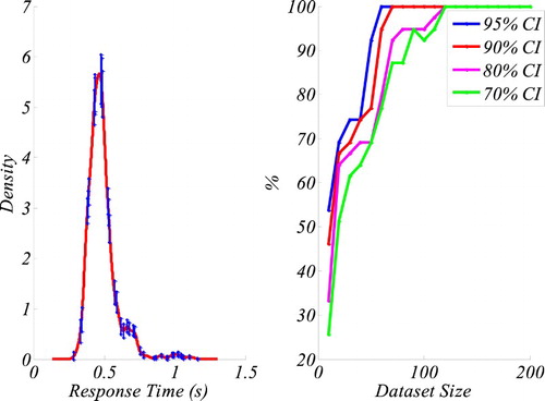
The target distribution was based on Wolfe et al.’s (2010) dataset as it contains a good number of trials in each condition (500). From this dataset we used the data from the conjunction search, Participant 1, display size 3. Since oKDE varies the number of kernels, we had to modify Van Zandt’s (2000) procedure. In order to find an appropriate comparison, we used an important property of oKDE. It is possible to characterize an entire KDE (and consequently the target distribution) by a series of “sigma points”. Hence, if another KDE has similar probability values at these sigma points, this new KDE represents a similar distribution (see Figure 4 for an illustration of sigma points; see Kristan et al., 2011, for details on sigma points). In order to determine these sigma points we fitted a KDE to Wolfe et al.’s (2010) dataset. This fit resulted in 13 kernels and 39 sigma points (see Figure 5). To test whether a KDE based on fewer data points still follows the shape of the distribution of the larger dataset, we also conducted a statistical test at each sigma point similar to Van Zandt (2000). Note that this is a somewhat more stringent test than Van Zandt’s (2000), as these sigma points represent a more complete description of the data than the peaks of kernels. Thus we first established the variation of probabilities (confidence interval) at the sigma points by employing a bootstrap method. We bootstrapped 1000-times the large dataset and fitted a KDE to each sample. We used these KDE to determine the confidence intervals at each sigma point (see Figure 5). These confidence intervals were used to determine whether a KDE from a smaller dataset is significantly different from the target distribution at these points. Subsequently, we created smaller datasets (Size: 10, 20, 30, etc.) by sampling from Wolfe et al.’s (2011) data set with replacement. For each data set size, we repeated this 1000 times and fitted a KDE to the smaller data set. Finally, we determined the percentage of values that fell into the confidence intervals at the sigma points. Figure III.1 shows the result of this assessment for different confidence intervals. With a data set size of 50, all KDEs fall into the 95% confidence interval. If a more conservative criterion is applied (i.e., a narrower confidence interval such as a 70% confidence interval) then 120 trials are needed to match the target distribution. These results suggest that oKDE is more powerful as the Silverman-KDE, as Van Zandt (2000) found only an around 80% match for 10,000 trials with the Silverman-KDE. However, given the methodological difference the results are difficult to compare directly. A more detailed comparison goes beyond the scope of this article. Nevertheless, our results indicate that oKDE is highly suitable for representing the dataset (100 trials per condition) used here.

Figure III.1. The graph on the left shows the KDE of the original data with 70% confidence intervals (CI) at the sigma points. The graph on right shows the percentage of KDEs from different dataset sizes falling into the confidence intervals. The results indicate that for a 95% CI, data sets as small as 50 data points produce a 100% accurate representation of the original distribution.

References

- Anderson, G. M., Heinke, D., & Humphreys, G. W. (2010). Featural guidance in conjunction search: The contrast between orientation and color. Journal of Experimental Psychology: Human Perception and Performance, 36(5), 1108–1127. doi:10.1037/a0017179.
- Balota, D. A., & Yap, M. J. (2011). Moving beyond the mean in studies of mental chronometry: The power of response time distributional analyses. Current Directions in Psychological Science, 20, 160–166. doi:10.1177/0963721411408885.
- Beaumont, M. A. (2010). Approximate Bayesian computation in evolution and ecology. Annual Review of Ecology, Evolution, and Systematics, 41, 379–406. doi: 10.1146/annurev-ecolsys-102209-144621
- ter Braak, C. J. F. (2006). A Markov chain Monte Carlo version of the genetic algorithm Differential Evolution: Easy Bayesian computing for real parameter spaces. Statistics and Computing, 16, 239–249. doi: 10.1007/s11222-006-8769-1
- Bruce, N. D. B., & Tsotsos, J. K. (2009). Saliency, attention, and visual search: An information theoretic approach. Journal of Vision, 9, 1–24. Retrieved from http://www.journalofvision.org/content/9/3/5, doi: 10.1167/9.3.5.
- Bundesen, C. (1990). A theory of visual attention. Psychological Review, 97(4), 523–547. doi:10.1037/0033-295X.97.4.523.
- Busemeyer, J. R., & Diederich, A. (2010). Cognitive modelling. Thousand Oaks, CA: Sage.
- Cousineau, D. (2005). Confidence intervals in within-subject designs: A simpler solution to Loftus and Masson’s method. Tutorials in Quantitative Methods for Psychology, 1(1), 4–10. doi: 10.20982/tqmp.01.1.p004
- Desimone, R., & Duncan, J. (1995). Neural mechanisms of selective visual attention. Annual Review of Neuroscience, 18, 193–222. doi: 10.1146/annurev.ne.18.030195.001205
- Duncan, J., & Humphreys, G. W. (1989). Visual search and stimulus similarity. Psychological Review, 96, 433–458. doi: 10.1037/0033-295X.96.3.433
- Duncan, J., Humphreys, G. W., & Ward, R. (1997). Competitive brain activity in visual attention. Current Opinion in Neurobiology, 7, 255–261. doi: 10.1016/S0959-4388(97)80014-1
- Eckstein, M. P. (2011). Visual search: A retrospective. Journal of Vision, 11(5), 14–14. doi:10.1167/11.5.14.
- Egeth, H., Jonides, J., & Wall, S. (1972). Parallel processing of multielement displays. Cognitive Psychology, 3, 674–698. doi:10.1016/0010-0285(72)90026-6.
- Egly, R., Driver, J., & Rafal, R. D. (1994). Shifting visual attention between objects and locations: Evidence from normal and parietal lesion subjects. Journal of Experimental Psychology: General, 123(2), 161–177. doi: 10.1037/0096-3445.123.2.161
- Heathcote, A., Brown, S. D., & Mewhort, D. J. (2002). Quantile maximum likelihood estimation of response time distributions. Psychonomic Bulletin and Review, 9, 394–401. doi: 10.3758/BF03196299
- Heinke, D., & Backhaus, A. (2011). Modeling visual search with the Selective Attention for Identification model (VS-SAIM): A novel explanation for visual search asymmetries. Cognitive Computation, 3(1), 185–205. doi: 10.1007/s12559-010-9076-x
- Heinke, D., & Humphreys, G. W. (2003). Attention, spatial representation and visual neglect: Simulating emergent attention and spatial memory in the Selective Attention for Identification Model (SAIM). Psychological Review, 110(1), 29–87. doi: 10.1037/0033-295X.110.1.29
- Hulleman, J., & Olivers, C. N. L. (2016). The impending demise of the item in visual search. Behaverial Brain Science. doi:10.1017/S0140525X15002794
- Humphreys, G. W., & Müller, H. J. (1993). SEarch via recursive rejection (SERR): A connectionist model of visual search. Cognitive Psychology, 25, 43–110. doi: 10.1006/cogp.1993.1002
- Itti, L., Koch, C., & Niebur, E. (1998). A model of saliency-based visual attention for rapid scene analysis. IEEE Transactions on Pattern Analysis and Machine Intelligence, 20(11), 1254–1259. doi: 10.1109/34.730558.
- Koch, C., & Ullman, S. (1985). Shifts in selective visual attention: towards the underlying neural circuitry. Human Neurobiology, 4, 219–227.
- Kristan, M., Leonardis, A., & Skočaj, D. (2011). Multivariate online kernel density estimation with Gaussian kernels. Pattern Recognition, 44(10), 2630–2642. doi: 10.1016/j.patcog.2011.03.019
- Kwak, H., Dagenbach, D., & Egeth, H. (1991). Further evidence for a time-independent shift of the focus of attention. Perception and Psychophysics, 49(5), 473–480. doi: 10.3758/BF03212181
- Leys, C., Ley, C., Klein, O., Bernard, P., & Licata, L. (2013). Detecting outliers: Do not use standard deviation around the mean, use absolute deviation around the median. Journal of Experimental Social Psychology, 49(4), 764–766. doi: 10.1016/j.jesp.2013.03.013
- Lin, Y-S., Heinke, D., & Humphreys, G. W. (2015). Modeling visual search using three-parameter probability functions in a hierarchical Bayesian framework. Attention, Perception, & Psychophysics, 77(3), 985–1010. doi: 10.3758/s13414-014-0825-x
- Maljkovic, V., & Nakayama, K. (2000). Priming of popout: III. A short-term implicit memorysystem beneficial for rapid target selection. Visual Cognition, 7, 571–595. doi: 10.1080/135062800407202
- Mavritsaki, E., Heinke, D., Allen, H., Deco, G., & Humphreys, G. W. (2011). Bridging the gap between physiology and behavior: Evidence from the sSoTS model of human visual attention. Psychological Review, 118(1), 3–41. doi: 10.1037/a0021868
- Mavritsaki, E., Heinke, D., Humphreys, G. W., & Deco, G. (2006). A computational model of visual marking using an interconnected network of spiking neurons: The spiking search over time & space model (sSoTS). Journal of Physiology-Paris, 100(1/2/3), 110–124. doi: 10.1016/j.jphysparis.2006.09.003
- Moran, R., Zehetleitner, M., Mueller, H. J., & Usher, M. (2013). Competitive guided search: Meeting the challenge of benchmark RT distributions. Journal of Vision, 13(8), 24–24. doi: 10.1167/13.8.24
- Müller-Plath, G., & Elsner, K. (2007). Space-based and object-based capacity limitations in visual search. Visual Cognition, 15(5), 599–634. DOI:10.1080/13506280600845572.
- Nelder, J. A., & Mead, R. (1965). A simplex method for function minimization. The Computer Journal, 7, 308–313. doi:10.1093/comjnl/7.4.308.
- Palmer, E. M., Horowitz, T. S., Torralba, A., & Wolfe, J. M. (2011). What are the shapes of response time distributions in visual search? Journal of Experimental Psychology: Human Perception and Performance, 37, 58–71.
- Ratcliff, R. (1978). A theory of memory retrieval. Psychological Review, 85(2), 59–108. doi: 10.1037/0033-295X.85.2.59
- Silverman, B. W. (1986). Density estimation for statistics and data analysis. London: Chapman and Hall.
- Storn, R., & Price, K. (1997). Differential evolution–a simple and efficient heuristic for global optimization over continuous spaces. Journal of Global Optimization, 11(4), 341–359. doi: 10.1023/A:1008202821328
- Townsend, J. T., & Ashby, F. G. (1984). Measurement scales and statistics: The misconception misconceived. Psychological Bulletin, 96(2), 394–401. doi: 10.1037/0033-2909.96.2.394
- Townsend, J. T., & Nozawa, G. (1995). Spatio-temporal properties of elementary perception: An investigation of parallel, serial, and coactive theories. Journal of Mathematical Psychology, 39, 321–359. doi: 10.1006/jmps.1995.1033.
- Treisman, A., & Gelade, G. (1980). A feature-integration theory of attention. Cognitive Psychology, 12, 97–136. doi: 10.1016/0010-0285(80)90005-5
- Treisman, A., & Gormican, S. (1988). Feature analysis in early vision: Evidence from search asymmetries. Psychological Review, 95, 15–48. doi: 10.1037/0033-295X.95.1.15
- Turner, B. M., & Sederberg, P. B. (2014). A generalized, likelihood-free method for posterior estimation. Psychonomic Bulletin & Review, 21(2), 227–250. doi: 10.3758/s13423-013-0530-0
- Turner, B. M., Sederberg, P. B., Brown, S. D., & Steyvers, M. (2013). A method for efficiently sampling from distributions with correlated dimensions. Psychological Methods, 18, 368–384. doi: 10.1037/a0032222
- Usher, M., & McClelland, J. L. (2001). The time course of perceptual choice: The leaky, competing accumulator model. Psychological Review, 108(3), 550–592. doi: 10.1037/0033-295X.108.3.550
- Van Zandt, T. (2000). How to fit a response time distribution. Psychonomic Bulletin and Review, 7, 424–465. doi: 10.3758/BF03214357
- Wertheimer, M. (1923). Untersuchungen zur Lehre von der Gestalt. II. Psychologische Forschung, 4, 301–350. doi: 10.1007/BF00410640
- Wickelgren, W. A. (1977). Speed–accuracy tradeoff and information processing dynamics. Acta Psychologica, 41, 67–85. doi: 10.1016/0001-6918(77)90012-9
- Wolfe, J. M. (1994). Guided search 2.0 a revised model of visual search. Psychonomic Bulletin & Review, 1(2), 202–238. doi: 10.3758/BF03200774
- Wolfe, J. M. (1998). Visual search. In H. Pashler (Ed.), Attention (Vol. 1, pp. 13–73). London: University College London Press.
- Wolfe, J. M. (2007). Guided search 4.0. In W. D. Gray (Ed.), Integrated models of cognitive systems (cognitive models and architectures) (pp. 99–120). Oxford: Integrated Models of Cognitive Systems.
- Wolfe, J. M., Cave, K. R., & Franzel, S. L. (1989). Guided search: An alternative to the feature integration model for visual search. Journal of Experimental Psychology: Human Perception and Performance, 15, 419–433.
- Wolfe, J. M., Palmer, E. M., & Horowitz, T. S. (2010). Reaction time distributions constrain models of visual search. Vision Research, 50(14), 1304–1311. doi: 10.1016/j.visres.2009.11.002
- Woodgate, P. J., Strauss, S., Sami, S. A., & Heinke, D. (2015). Motor cortex guides selection of predictable movement targets. Behavioural Brain Research, 287, 238–246. doi: 10.1016/j.bbr.2015.03.057.
- Zhao, Y., Heinke, D., Ivanoff, J., Klein, M. K., & Humphreys, G. W. (2011). Two components in IOR: Evidence for response bias and perceptual processing delays using the SAT methodology. Attention Perception & Psychophysics, 73(7), 2143–2159. doi: 10.3758/s13414-011-0181-z
- Zhao, Y., Humphreys, G. W., & Heinke, D. (2012). A biased-competition approach to spatial cueing: Combining empirical studies and computational modelling. Visual Cognition, 20(2), 170–210. doi: 10.1080/13506285.2012.655806
Appendices
Appendix I
SAIM-WTA
The gamma-parameter in DE-MCMC was set toAppendix II