Pension plan solvency and extreme market movements: a regime switching approach

Abstract

We develop and test a new approach to assess defined benefit (DB) pension plan solvency risk in the presence of extreme market movements. Our method captures both the ‘fat-tailed’ nature of asset returns and their correlation with discount rate changes. We show that the standard assumption of constant discount rates leads to dramatic underestimation of future projections of pension plan solvency risk. Failing to incorporate leptokurtosis into asset returns also leads to downward biased estimates of risk, but this is less pronounced than the time-varying discount rate effect. Further modifying the model to capture the correlation between asset returns and the discount rate provides additional improvements in the projection of future pension plan solvency. This reduces the perceived future risk of underfunding because of the negative correlation between interest rate changes and asset returns. These results have important implications for those with responsibility for balancing risk against expected return when seeking to improve the current poor funding positions of DB pension schemes.

Keywords:

• pension fund solvency
• leptokurtosis
• risk estimation
• value at risk

JEL Classification:

• G17
• G23
• C58

1. Introduction

The purpose of this paper is to investigate defined benefit (DB) pension plan solvency risk and propose a new approach to more accurately measure the solvency position of a pension plan in the presence of extreme market movements. Since the start of the credit crisis, the aggregate funding position of DB pension schemes in the UK has swung dramatically between deficit and surplus. For example, the UK Pension Protection Fund PPF 7800 index revealed an aggregate funding surplus of £161bn in June 2007, which turned into a deficit of £182bn by March 2009. By January 2011 this had returned to a £50bn surplus before swinging back to a deficit of £317bn in May 2012. Latest figures (May 2014) show these funds are still, on aggregate, £118.2bn in deficit; a funding ratio of 90.8%, with 71% of schemes underfunded.¹

We present detailed projections of how the solvency position of DB schemes might evolve in the future. At the aggregate level, this work is of relevance to the Pension Protection Fund and macro-prudential regulators. At the individual fund level, our results should be of interest to those involved in pension fund management including actuaries, trustees and sponsors.

The methods that we employ capture three key features of the data that recent market conditions have highlighted. First, we allow for the fat-tailed nature of asset returns, particularly on the downside, that has been so clearly revealed in recent years (Frankland et al. 2008). Second, we recognise that discount rates change over time (Cochrane 2011). This phenomena has been observed between March 2009 and May 2012, when the aggregate funding position of UK DB schemes worsened by more than £100bn at a time when asset values actually increased from £776bn to £1025bn. This was due to even greater rises (from £956bn to £1323bn) in the present value of future liabilities as a result of a decline in gilt yields. Finally, we capture the dynamic correlation between discount rates and asset returns. Unconditionally, discount rate changes are negatively correlated with asset returns as both bond and equity prices tend to rise when interest rates are falling. This means that there is a positive correlation between the present value of liabilities and the market value of assets. This, though, is not always the case. Between June 2007 and March 2009 the aggregate value of DB assets fell by approximately 6%, from £830bn to £776bn, while simultaneously, the present value of future liabilities rose by over 40%, from £668bn to £956bn.

Our core empirical model involves the use of multivariate Gaussian regime switching models. This framework is well suited to modelling asset returns and extreme market events (see Ang and Timmermann 2011 for a recent review). Not only does it capture leptokurtosis in asset returns, but it has also been shown to accurately capture the increased correlations between asset returns that often occur in bear markets (Ang and Bekaert 2002).

The paper is related to two streams of the existing literature. The first examines optimal contribution rates and asset allocation decisions for DB pension plans. Josa-Fombellida and Roncón-Zapatero (2011), for example, consider the optimal portfolio for minimising the terminal solvency risk of a DB scheme in the presence of stochastic interest rates, asset returns and benefits in a non-regime switching environment. Our specific focus, though, is somewhat different. Rather than determining what fund managers ‘should’ do, we provide a general risk framework for current decisions regardless of whether or not they conform to what academics might view as being theoretically optimal. By removing the need to optimise, we are able to deal with more complex statistical representations of the data than is common in this literature. Apart from Fraudendorfer, Jackoby, and Schwendener (2007), Markov switching models have not, to our knowledge, been widely used when determining optimal DB pension plan portfolios. This is despite the fact that they have been applied in more general asset allocation contexts by, for example, Ang and Bekaert (2002), Zhou and Yin (2003), Guidolin and Timmerman (2007, 2008) and Shen and Siu (2012).

Our work is perhaps more closely related to value-at-risk (VaR) problems. Here, Markov switching models have been used by a number of authors including Billio and Pelizzon (2000), Guidolin and Timmerman (2006b) and Taamouti (2009). Kawata and Kijima (2007) demonstrate that these models estimate 1% VaR levels for portfolios better than many alternative approaches. Ferstl and Weissensteiner (2011) evaluate the optimal portfolio that will minimise the conditional VaR for a DB pension scheme, but again they do not consider regime switching within their setting.

Our main result is that the assessed risk of pension scheme underfunding is highly dependent on the precise specification of the econometric process driving asset returns and changes in the discount rate. Given that most of the recent volatility in pension scheme funding has arisen from changes in the present value of liabilities, it is perhaps no surprise that incorporating stochasticity in the discount rate significantly increases the assessed level of future funding risk. Similarly, incorporating leptokurtosis into asset returns increases the calculated probability of a fund going into deficit in future, although this has a smaller impact than the stochasticity of the discount rate. Finally, because of the unconditional negative correlation between asset returns and interest rate changes, incorporating this relationship reduces perceived future funding risk. This is true even within our Markov switching model, as even in the crash state this correlation remains negative. Although this contrasts with the situation between June 2007 and March 2009, it is representative of the more recent post-crisis period.

The conclusion we draw is that pension fund stakeholders need models at least as sophisticated as the ones presented here if they are to fully appreciate future solvency risk. Techniques that are easier to estimate and more pragmatic are likely to lead to materially incorrect inferences and poor decision-making by regulators and those involved in pension fund management.

Our paper proceeds as follows. In Section 2, we describe the economic environment and illustrative portfolio that will be used to generate our results. In Section 3, we consider the funding risk of our illustrative portfolio in a single-state model, where portfolio returns are lognormally distributed. In Section 4, we allow for extreme market movements by modelling asset returns as a Markov switching process. Section 5 considers four extensions: the use of a more sophisticated liability model, an analysis of how well the different models explain the reduction in aggregate DB pension plan funding during the credit crisis, the impact of parameter uncertainty on our findings and the use of more parsimonious Markov models. Section 6 concludes.

2. Model framework

We consider a DB pension plan that has assets under management and a future stream of liabilities that must be met. We assume the scheme is based in the UK and payouts are sterling denominated. It invests in N=5 asset classes. Four of the asset classes are equities (UK, non-UK Europe, USA and Japan) and the remaining asset class consists of UK government bonds (gilts). The assets have a combined market value at time t of V_t and we use PV_t(L) to denote the present value of the future liabilities as calculated at time t. The model is normalised by setting V₀=1. The variable that the stakeholders of this fund are interested in is z_t, which is the funding ratio of the scheme: The scheme is fully (under)funded if z_t>(<)0. Our central research question is to examine the statistical distribution of z_t, whose properties will be sensitive to modelling choices concerning V_t and PV_t(L). This paper is therefore an extension of other studies that examine pension scheme funding ratios (for example, Hoevenaars et al. 2008; Leibowitz, Kogelman, and Bader 1994; Sharp and Tint 1990). In particular, we develop sophisticated approaches that assess the probability that a scheme will be underfunded at a future time t under current investment and contribution policies; .

This is a pressing issue. A recent survey of major employers (Mercer/ICAEW 2012) found that nearly all companies (98%) viewed the management of DB pension scheme risk as a priority. For two-fifths of firms it was either their most important, or one of the most important, risk management issues with ‘deficit funding and deficit reduction (being) one of the most frequently cited concerns’ (Mercer/ICAEW 2012, 2). This may be because ‘rising deficits are forcing some employers to make substantial additional contributions to schemes, which is diverting funds away from business investment and ultimately, economic growth’ (D.W.P 2013, 3). In addition, under International Accounting Standard 19, there is a requirement for companies to place on their balance sheet their net pension scheme funding position. Deficits therefore weaken firms’ abilities to borrow at competitive rates. Finally, schemes must pay levies to the PPF and the greater the level of underfunding the higher is the levy. This creates positive feedbacks in risk position. Deficits are also of concern to pension fund members. Sponsors are increasingly unwilling to take on investment risk, leading to a dramatic decline in UK membership of DB plans. In addition, deficits have, in many instances, contributed towards a deterioration in pension terms for those members who remain in such schemes. This has generally been seen through some combination of higher employee contributions, lower future benefits and/or later retirement dates.²

By identifying the probability of future deficits under a ‘business as usual’ scenario, we are providing an early warning mechanism for stakeholders that will identify the possibility that a fund will need to undertake recovery measures in the future. This will help guide investment policy, influence risk management strategies and prevent companies from taking unwarranted pension fund holidays due to a mis-estimation of their schemes’ risk. The problem we face is related, but not identical, to a VaR calculation. In the latter case, for some confidence interval α the fund manager finds the value of future assets VaR_t that is the solution to the equation: . In the situation considered in this paper, there are two adjustments to this equation. First, instead of fixing α, the value of VaR_t is determined and then α is derived as a consequence. That is, we determine probabilities of falling into deficit rather than asset values associated with predetermined left-hand tail probabilities. Second, our research question can be rephrased as assessing , where both the left- and right-hand sides of the equation are stochastic and correlated. Therefore, our work can be seen as being complementary to the work of Billio and Pelizzon (2000), Guidolin and Timmerman (2006b), Kawata and Kijima (2007) and others.

Following Leibowitz, Kogelman, and Bader (1994), we define the per-period funding ratio return (FRR_t) over the interval [0, t] by

As they show, an important property of this variable is that it is independent of the initial funding level. Intuitively, this is because 1+z_t is a returns multiple of 1+z₀, and therefore, the ratio of these two variables is not a function of z₀. Therefore, an alternate interpretation of our results is that , where z₀ is the opening surplus funding level that we choose for our calibrations described below (z₀=0.15). This will hold for any fund, whatever its current surplus or deficit, provided its asset allocations match those in our models.

2.1. Modelling of assets

In order to assess future solvency risk, historical data are used to determine the relevant underlying statistical relationships and it is then assumed that these will not change in the future.³ Calibration is undertaken using monthly data from January 1970 to December 2010. For UK equities, data for the FTSE All Share total returns index are taken from Datastream. All other data for the asset side of the balance sheet are taken from Global Financial Data. These are the UK 10-year Government Bond total return index, S&P500 total returns index, Japanese Topix total returns index and MSCI Europe total returns index. As the scheme is UK-based, all returns have been adjusted for currency fluctuations and are calculated in sterling terms. In Table 1, we present summary statistics for the total monthly lognormal returns, where I_nτ is the total returns index of asset class n, to each series that we consider on the asset side of the balance sheet.

Table 1.  Summary statistics for the data.

	Mean	Standard deviation (%)	Skewness (%)	Excess kurtosis
Panel A: First four moments of asset returns
UK equity returns	0.809	5.730	−0.710	7.436
US equity returns	0.895	5.264	−0.637	2.448
European equity returns	0.936	4.716	−1.010	3.904
UK gilt returns	0.784	1.742	0.446	2.424
Japanese equity returns	0.833	6.012	−0.054	0.517
Panel B: Correlation coefficients (with assets in the same order)
1.00	0.56	0.83	0.25	0.33
	1.00	0.70	0.02	0.40
		1.00	0.15	0.47
			1.00	0.06
				1.00

Notes: This table presents the first four moments of total monthly asset returns in Panel A, and the correlation coefficients between these different asset returns in Panel B, for five asset classes. These summary statistics are calculated using data for the period January 1970 to December 2010. All returns are calculated in sterling terms.

The pension scheme invests a proportion of its total wealth w_n in each of the asset classes with and assets ordered as in Table 1 (n=1 for UK equities, n=4 for UK gilts, etc.). Let w be the N-vector with elements w_n. We assume that and is fixed across time with weights rebalanced each period.⁴

2.2. Modelling of liabilities

The liability structure of a DB pension scheme is highly complex. Among other factors, future payouts from the scheme will depend on longevity risk, age of retirement, salary growth, additional contributions and other contribution rate changes, taxation changes, and withdrawals from and additions to the scheme. As the central focus of this paper is to understand the impact of different econometric choices on assessed future funding risk, we in the main assume a stylised form for expected future liabilities of the DB scheme. In our main calibrations, at all times liabilities stretch over the next 30 years. The first expected liability, in one year's time, is C₁. Following that, the liabilities are expected to grow at a fixed inflation rate i. This leads to the following schedule of expected future liabilities:

Given this schedule, the present value of liabilities that will be calculated at any time t is given by the growth annuity formula where is the 30-year growth annuity value based on the rate, r_ft, that is used at time t to determine the present value of future liabilities: The initial expected cash flow, C₁, is set so that , where z₀ represents the initial solvency level of the scheme expressed so that, with V₀=1, the fund has a present value of future liabilities of . For our illustrative example, we set . We also assume that there are no net contributions to the asset side of the balance sheet after time zero as new contributions exactly offset fund payouts. It should be stressed that these assumptions are for simplicity of exposition only. The processes that we describe could easily be extended to more complex cash flow dynamics and net inflows/outflows from the fund. We return to this issue in Section 5.1. In order to calculate the present value of the liabilities, we use the 10-year UK gilt yield, rather than the AA corporate bond rate, as given by Datastream.⁵ We estimate the probability that z_t<0 for all t up to a horizon of 30 years based on six different econometric specifications of the data. The first three take a simple one-state lognormal process for asset returns, while the last three incorporate Markov regime switching. In Models 1 and 4, it is assumed that the discount rate is fixed at its current level: r_ft=r_f0 for all t. All other models incorporate an AR(1) or, equivalently, discrete-time Ornstein–Uhlenbeck (O–U) model for the discount rate. In Models 2 and 5, the discount rate process is assumed to be independent of asset returns. Models 3 and 6, however, incorporate the observed correlation between discount rate changes and portfolio returns.

3. Modelling solvency risk: single-state setting

Let be the single-period logarithmic return to the portfolio that is held by the pension fund. Throughout this section, we assume that r_pτ is independently and identically normally distributed (i.i.n.d.), . There are a number of weaknesses in this approach. First, it does not capture the higher moments of asset returns and in particular their ‘fat-tailed’ properties that are clearly present in the summary statistics of the data presented in Table 1. Consequently, the model underestimates extreme market events and the true spread of possible future portfolio values. Second, it is well known that asset return variances are time-varying, and this is not captured within the single-state setting. We address these limitations later in the paper.

The variable of interest is the probability that the DB scheme becomes underfunded: or equivalently, . As under the i.i.n.d. assumption ln (V_t) = = , this becomes a standard z-score problem.

We begin with Model 1, which is the simplest specification. We impose the condition that the risk-free rate will remain constant at its current value, r_ft=r_f0 for all t, which we set at the observed gilt yield in December 2010; . In this case, is non-stochastic and

where Φ (·) is the cumulative distribution function of a standard normal distribution. Model 2 relaxes the constant discount rate assumption by now letting it follow an independent AR(1), or discrete-time O–U, process. The continuous-time form of this process, as suggested initially by Vaşicek (1977), has been used in a related context by Josa-Fombellida and Roncón-Zapatero (2011): where θ=b, and . This gives the AR(1) process an economic interpretation; represents the long-run interest rate value to which the discount rate mean reverts and θ is the parameter value that determines the speed of the mean reversion. While more sophisticated interest rate models are available, the AR(1) specification is highly analytically tractable. The probability density function of r_ft, f(r_ft), conditional on the current discount rate, r_f0, is normally distributed with mean E[r_ft] and variance : In addition, the transformed variable x_t: is i.i.n.d. These properties are useful in later, more general, models. Basing our parameterisations on the de-annualised monthly 10-year UK gilt yield for the interval January 1970 to December 2010, we derive estimates of , and . The annualised value of and the estimated half-life of this process is months, or 16 years. This implies that the speed of mean reversion in the model is very low.

As both the total return index for the fixed income asset and x_t are based on 10-year UK Treasury bond data, we would anticipate that these two variables should be highly negatively correlated. The estimated correlation coefficient over the total sample is −85.8%, and in all months the sign of x_t is opposite to the sign of the gilt's total return. As a consequence, by constructing a pension fund heavily weighted in the fixed income asset, much of the solvency risk can be hedged. However, such portfolios do not conform with observed average pension fund behaviour (see Note 4), primarily because this strategy does not, in the opinion of most pension fund managers, optimally balance risk against expected return.

By the law of total probability, . When the portfolio return is independent of the discount rate process, this is equivalent to which can be evaluated by numerical integration.

In Model 3, we continue to assume that portfolio returns are one-state lognormally distributed and discount rates are characterised by the AR(1) process. Now, though, we allow for the observed correlation between the discount rate, r_ft, and the logarithmic portfolio value, at time t. By backward iteration: Therefore, When there is only one state, , where ρ is the correlation between r_pt and e_t which is a constant. Therefore, and the correlation between and r_ft, ρ_t is Applying a well-known result for the conditional distribution of bivariate normal variables: and so Again, this can be evaluated by numerical integration.

In order to calibrate m and σ² we make the simplifying assumption that . Strictly speaking, it is simple portfolio returns that are the weighted average of simple individual asset returns and, therefore, taking weighted averages of logarithmic returns in this way is an approximation. However, when returns are small, as is generally the case with monthly data, this approximation works well. Unreported results, where we run simulations at the individual asset level, suggest that our conclusions are robust to this assumption. In this case, if the individual logarithmic asset returns are i.i.n.d., then r_pt will also be i.i.n.d. as required. Let μ_τ denote the N-vector with elements and Σ_τ denote the N×N matrix with elements . For the calibration exercise, we set and for all τ, as given in Table 1, resulting in and . In Figure 1, we present the results from the three models when the inflation rate . It can be seen that the probability of default first rises and then dissipates quickly in each case. This is because the expected return to the portfolio is substantially above the assumed fixed inflation rate of 4%. Therefore, the expected returns effect quickly dominates the stochasticity of the asset returns and discount rate processes.

Fig. 1. This graph presents the probability that the scheme will be underfunded at time t; Prob(z_t<0). Results are presented for three models, all of which assume that portfolio returns are i.i.n.d. In Model 1, the discount rate is fixed at its current level. In Model 2, the discount rate is stochastic but independent of the portfolio return. Model 3 allows for the correlation between the discount rate and the portfolio return process.

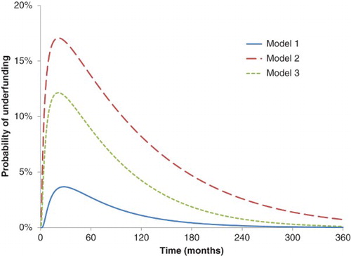
Under Model 1, where the discount rate is fixed, the maximal probability of becoming underfunded is relatively low; around 4% after two years and four months. This then drops away quite rapidly.

Under Model 2, the results are markedly different with a much higher maximal probability of underfunding, which now lies at approximately 17% after one year and nine months. There are three key causes for this, two of which amplify the difference and the third of which reduces it. First, there is now a probability that discount rates will fall substantially. To illustrate, suppose momentarily that the portfolio will deliver a non-stochastic return of mt over the next 12 months. For the pension scheme now to be underfunded in one year: Given and , this corresponds to . Based on the calibrated one-state O–U model, this movement is not unlikely with a p-value of over 12%. Therefore, even if there is no uncertainty over asset returns, the interest rate stochasticity effect is highly significant.

Second, there is a Jensen's inequality effect that also increases the perceived solvency risk. When interest rates are stochastic the expected net present value is greater than the present value calculated at the expected discount rate. To illustrate this, suppose that the discount rate in five years, r_f5, might equal 8% or 2% with equal probability. In this case, . By contrast, . This effect has been very heavily documented in environmental economics, where it leads to a declining schedule of discount rates with increasing time horizon (Weitzman 2001) and, in turn, a higher social cost of carbon. In the context given here, after 12 months the O–U process leads to estimates and . The growth annuity value at the expected discount rate . However, when we run a simulation of 1,000,000 drawings of r_f1 from the relevant normal distribution, . In Figure 2, we present a comparison of these two types of annuity value for t up to 360 months. This demonstrates how economically significant this effect can be. Therefore, ignoring uncertainty about the discount rates at future time t will lead to an underestimate of the expected growth annuity value at time t, and thus an understatement of the expected present value of future liabilities that will prevail at that time.

Fig. 2. This graph presents the growth annuity value for T=30 years for t up to 360 months. The ‘Known rf’ line assumes that r_ft=E[r_ft] with certainty, where E[r_ft] is determined by the discrete-time O–U process described in the body of the paper. The ‘Stochastic rf’ is calculated as the average growth annuity value determined over 1,000,000 simulations when r_ft is drawn at random from this distribution.

The third, offsetting, effect is that the long-run equilibrium annualised discount rate, on an annualised basis, is considerably higher than the initial risk-free rate of . This implies that the term structure of expected discount rates is upward sloping, reducing the growth annuity value estimates in the future. This feature is clearly evident from the ‘Known rf’ line in Figure 2. We would expect the differences between Models 1 and 2 to be greater than presented here when the term structure is flat. Figure 1 also presents results for Model 3, which allows for the covariance between discount rates and asset returns. This somewhat reduces the perceived pension fund solvency risk, with a maximal probability of underfunding now being at about 13% at one year and nine months. The reason for this is that, in general, asset returns are negatively correlated with the discount rate, with unconditional correlation between r_pt and e_t of . This is most obviously driven by UK gilts, which make up 40% of the overall portfolio. As might be expected, the total return on this asset class is highly negatively correlated over the sample period with the discount rate . In addition, UK equity returns are also negatively correlated with bond yields . Therefore, the market value of assets and the present value of liabilities tend to move up and down in tandem, providing a natural hedging effect for pension fund stakeholders.

4. Modelling solvency risk: four-state setting

To overcome the weaknesses of the traditional one-state lognormal model of portfolio returns, we extend our analysis to incorporate extreme events into the analysis. There are a number of techniques available to do this, of which perhaps the two most commonly employed are extreme value theory (EVT) models that incorporate copulas and Markov regime switching models. Within the VaR literature both techniques have been used; for example, Embrechts, Resnick, and Samorodnitsky (1999) and Longin (1999) use EVT, while Guidolin and Timmerman (2006b) and Kawata and Kijima (2007) employ Markov models. There is no compelling reason for choosing one of these methods over the other when addressing the problem at hand. Indeed, Kemp (2011) demonstrates that any multivariate distribution, including those used in EVT, can be modelled arbitrarily accurately (except, perhaps, in the very far tail) by a distributional mixture of sufficiently many different multivariate normal distributions. Given the broad econometric similarities between the two approaches, in this paper, we have preferred Markov models primarily for pragmatic reasons. Under the UK Pension Regulator's Code of Practice 7, there is a requirement for trustees to understand the advice that they are given. Ang and Timmermann (2011, 1) observe that ‘the idea of regime changes is natural and intuitive’ and, as we will show below, the different states have a clear economic interpretation to which practitioners will naturally respond. Discussions with actuaries and pension fund managers also led us to believe that Markov models are easier to explain intuitively to pension scheme stakeholders than the EVT-copula alternative. In addition, we demonstrate below that these Markov models accurately capture much of the unconditional distribution of portfolio returns, including the observed leptokurtosis. Ang and Timmermann (2011) provide a detailed discussion of the many advantages of using this approach.

Given the statistical flexibility and ease of interpretation, it is perhaps no surprise that Markov models have been commonly employed throughout the economics and finance literature. For example, they have been used to capture structural breaks in the economy (see Hamilton 1989; Lam 1990; Raymond and Rich 1997; Storer and Van Audenrode 1995). They are also observed in a wide range of other settings, including time series generalised autoregressive conditional heteroskedasticity modelling (Hamilton and Susmel 1994); error correction (Psaradakis, Sola, and Spagnolo 2004) and causality (Psaradakis, Ravn, and Sola 2005). In addition to VaR and asset allocation, finance Markov switching has been used in option pricing (Boyle and Draviam 2007), bond pricing (Elliott and Siu 2009), foreign exchange modelling (Dueker and Neeley 2007) and elsewhere. In contrast to the previous models, it is now no longer assumed that μ_τ and Σ_τ are constant across time. Instead, the Markovian assumptions are that, at any time τ, the world lies in one of S states. We use the dummy variable for to denote the state that occurs at time τ. The probability we assign at time τ to the world being in state s at time τ+1, Prob, depends only on the state at time τ. A simple, fixed, transition probability matrix, M, can then be used to fully describe the stochastic way in which the prevailing state changes over time. The eigenvectors of M provide the ergodic probabilities, π_s, associated with each state, which can be interpreted as the proportion of time that the economy spends in each of the states over very long time periods.

Within each state, logarithmic asset returns, , are modelled as following a multivariate independent and identically distributed normal distribution with a vector of expected returns μ_s and variance–covariance matrix Σ_s. Within each state, the mean and standard deviation of logarithmic portfolio returns are again approximated by a normal distribution with means and variances and , respectively. Modelling alternatives are available. Elliott and Miao (2009), for example, allow the error terms to be Student's-t distributed within a Markov switching evaluation of VaR problems, thus introducing leptokurtosis within each state as well as by switching between states. Okimoto (2008) and Chollette, Heinen, and Valdesogo (2009) have recently presented combined regime switching with copula models. These more sophisticated models, though, increase the estimation difficulty, allow for less rich state processes, and reduce the number of asset classes that might reasonably be included within the estimation process. In addition, Kemp (2011) shows that nearly all upside fat-tailed behaviour and approximately one-half of downside fat-tailed behaviour of major Western developed equity markets can be explained purely by the presence of time-varying volatility without the need to invoke any non-normality in the conditional return distribution. Even with the Gaussian specification of a Markov switching process, there are a large number of parameters to be estimated. For each of the S states it is necessary to estimate N values of μ_s, N(N+1)/2 values of Σ_s, plus the S(S−1) degrees of freedom in M, giving a total of . We use a four-state (S=4) process throughout, which is consistent with the choice of Guidolin and Timmerman (2006a) for jointly capturing US stock and bond dynamics. In addition, both the Akaike and Bayesian information criteria show a preference for a four-state specification of the data employed here over either two or three states. This is sufficiently sophisticated to capture many of the broad statistical properties of the historical data, but is sufficiently limited so that, at 92, the number of parameters for estimation remains parsimonious.

In order to estimate this multivariate regime switching environment, we invoke the MSVARlib package in GAUSS written by Benoit Bellone. The code uses maximum-likelihood methods to estimate regimes in a vector autoregressive (VAR) framework. We estimate two Markov environments, both under the assumption that asset returns exhibit zero autocorrelation. The first incorporates the five asset classes alone and this characterisation of the data is used for Models 4 and 5. The second incorporates the variable x_t, which is also not autocorrelated, into the estimation process, giving six variables in all. This parameterisation is used for Model 6, our most sophisticated, as it captures the correlation between the discount rate process and asset returns within a Markov environment.

The MSVAR code would allow for the estimation of VAR regime switching processes. Single-state VAR models have been used in a related context by Hoevenaars et al. (2008) to investigate optimal strategic asset allocation for a pension fund with preferences based on the funding ratio and where there is a time-varying investment opportunity set. In unreported results, we have run estimations with a first-order VAR specification for some of our Markov switching models. This has no substantive impact on our results and comes at considerable computational cost. In addition, the presence of different states helps capture time variation in investment opportunities, albeit in a somewhat different way than a standard VAR model.

4.1. Markov estimates: five asset classes

Panel A of Table 2 presents the estimated summary statistics () for the monthly returns to our illustrative portfolio over each of the four states, with the ‘Correl’ column presenting the correlation between UK equity returns and gilt returns in each state. This panel also gives the ergodic probability, π_s, associated with each state. Panel B of Table 2 gives the transition probability matrix, M, where element . Of course in a Markov model where the investment opportunity set is time-varying, the theoretically optimal portfolio is dependent on the underlying state. However, we continue to keep the weights in our illustrative portfolio fixed through time and identical to those described above. This makes the impact of different modelling choices on our results more transparent. Again, though, it would be straightforward to extend this analysis to state-dependent weights.⁶

Table 2.  Summary statistics for the five-asset, four-state model.

Panel A: Portfolio returns in the four states
	Mean (%)		Standard deviation (%)		π (%)	Correl (%)
State 1	0.66		2.83		40.8	2.4
State 2	1.31		2.43		37.8	44.6
State 3	0.90		1.40		14.8	−7.6
State 4	−1.16		6.43		6.6	32.2
Panel B: Transition probability matrix
Panel C: Unconditional portfolio returns: summary statistics
	Model			Data
Mean	0.824%			0.830%
	[0.798%, 0.851%]			[0.757%, 0.903%]
Standard deviation	2.98%			2.96%
	[2.95%, 3.00%]			[2.79%, 3.16%]
Skewness	−0.562			−0.680
	[−0.648, −0.475]			[−0.896, −0.464]
Excess kurtosis	3.683			4.646
	[3.292, 4.080]			[4.213, 5.079]
Panel D: Future portfolio values: summary statistics
	Four state			One state
	T=5	T=10	T=30	T=5	T=10	T=30
Mean	1.71	2.93	26.98	1.69	2.84	23.16
Lower 2.5%	0.87	1.13	4.21	1.04	1.44	6.53
Upper 97.5%	2.80	6.05	98.28	2.58	5.13	60.17

Notes: This table presents summary statistics for the Markov switching environment with four states and five asset classes. Panel A provides details of portfolio returns in the four identified states, with π representing the ergodic probabilities and ‘Correl’ being the correlation between UK equity and gilt returns in each state. Panel B gives the transition probability matrix. Panel C provides summary statistics for the unconditional first four moments of asset returns generated from simulations of the Markov switching process, with 95% confidence intervals in parentheses. These are compared against the properties of the data. Panel D compares summary statistics for the future value of the illustrative portfolio, V_t, under the Markov switching model and the one-state lognormal model at different time horizons measured in years.

The four states have clear economic representation. State 1, which we define as the ‘low average returns state’ has average returns slightly below the unconditional expectation (0.66% vs. 0.83%) but is otherwise unexceptional. State 2 is the ‘bull state’ with annualised average returns of almost 16%. The average correlation between asset classes is relatively low in this state, giving portfolio volatility that is somewhat below the unconditional estimate. From the ergodic probabilities (the eigenvalues of M), the economy spends almost 80% of its time in one of these two states. State 3, the ‘low volatility state’, has close to average expected returns and correlations, but very low volatility. State 4, the most infrequent by occurring only 6.6% of the time, is the most interesting for our purposes. It is a clear ‘crash state’ with very high volatility, very high correlation between different asset classes and an annualised expected return of approximately . It is this state that captures the extreme market movements within our model. The transition matrix allows us to estimate the expected period of time in any one state before transition into an alternate state. This is given by (1−M_ii)⁻¹. This has values of approximately seven months for State 4 and over two years for all the other states. ‘Crash state’ 4 is most commonly entered from State 2 and also most commonly exits back into State 2.

To check the accuracy with which this four-state representation of the data captures the unconditional dynamics of portfolio returns, we simulate returns over 50,000 months. At time t=0, the initial state is chosen according to the ergodic probabilities. For each future time period, the state is calculated at random using the transition probability matrix, M. Within each state, the mean and standard deviation of logarithmic portfolio returns are again approximated by a normal distribution with means and variances and , respectively, which are reported in Panel A of Table 2. A single-period return is then constructed using a random number generator based on these parameter values and the first four moments of the returns across the 50,000 months are then calculated. This process is repeated 500 times, and the mean values of the first four moments across those 500 iterations are presented in Panel C of Table 2, together with lower 2.5% and upper 97.5% estimates from these simulations. These are compared against the estimated first four moments from the data with associated 95% confidence intervals.⁷

As is well known, conditional heteroskedasticity can lead to unconditional fat-tailed distributions. This is clearly observed here, where the excess kurtosis is statistically significantly above zero. This characterisation of the data still falls a little short of capturing all the leptokurtosis in the data, primarily because within each state returns continue to be generated by Gaussian distributions. A priori, we would expect that the presence of fat tails from this Markov switching environment would lead to wider 95% confidence intervals for the future asset value of the portfolio, V_t, than the one-state model. This would also be consistent with the findings of Kawata and Kijima (2007). To test this, we simulate forward the value of the portfolio, V_t, 10,000 times for 360 months. We can then compare these values for t=5, 10 and 30 years with those from the one-state model. These results are presented in Panel D of Table 2. As can be seen, there are significant differences. At a maturity of five years, the traditional model predicts with 97.5% confidence that the value of the portfolio will be at least 4% greater than the initial value. By contrast, the Markov switching model gives a 2.5% chance of a fall of 13%. The differences between the models become ever larger with increased time horizons.

4.2. Markov estimates: five asset classes and x_t

In Model 6 presented below, we include x_t as a sixth variable to be estimated in the Markov switching process. x_t is constructed by first estimating the parameter b over the whole sample and then treating this as the ‘true’ and time-invariant value. Within an O–U interpretation of the interest rate process, this is equivalent to having the speed of mean reversion, θ, constant across states but allowing both the long-run interest rate value and the volatility of the discount rate process, , to be state dependent. There are now 120 variables that need estimating.

The summary statistics for estimated portfolio returns in the four states are given in Panel A of Table 3, with a transition probability matrix in Panel B.

Table 3.  Summary statistics for the six-asset, four-state model.

Panel A: Portfolio returns in the four states
	Mean (%)	Standard deviation (%)	π (%)	(%)	Correl (%)
State 1	−1.90	5.67	6.0	−23.1	18.3
State 2	0.53	2.48	43.6	−11.8	−26.4
State 3	1.11	2.39	34.6	−52.3	48.0
State 4	1.77	3.10	15.7	−53.9	34.3
Panel B: Transition probability matrix
Panel C: Unconditional portfolio returns: summary statistics
	Model, rp		Data, rp	Model, xt	Data, xt
Mean	0.780%			1.20	1.65
	[0.754%, 0.803%]		0.830%	[0.98, 1.40]
Standard deviation	2.961%			26.13
	[2.937%, 2.986%]		2.963%	[25.89, 26.35]	28.58
Skewness	−0.467
	[−0.531, −0.408]		−0.680	–	–
Excess Kurtosis	2.366
	[2.091, 2.673]		4.646	–	–
Corr(rp, xt)	−37.7%
	[−38.7%, −36.7%]		−40.7%	–	–

Notes: This table presents summary statistics for the Markov switching environment with four-state and six-asset classes, including x_t which is a measure of the change in risk-free rate and that is formally defined in the body of the text. Panel A provides details of portfolio returns in the four identified states, with π representing the ergodic probabilities and ‘Correl’ being the correlation between UK equity and gilt returns in each state. Panel B gives the transition probability matrix. Panel C provides summary statistics for the unconditional first four moments of asset returns generated from simulations of the Markov switching process, with 95% confidence intervals in parentheses. These are compared against the properties of the data. In Panel C, all statistics for x_t have been multiplied by 10⁵.

There are clear similarities between States 2, 3 and 1 in this case with States 1 (‘low average returns state’), 2 (‘bull state’) and 4 (‘crash state’), respectively, in the previous parameterisation. What is particularly noticeable is that, even in the ‘crash state’ (now State 1), asset returns and the discount rate process remain negatively correlated, although at a lower absolute level than the unconditional average. This gives fund managers a natural hedge during market falls. While this is consistent with the post-crash period since March 2009, it does not reflect the simultaneous falls in discount rates and asset values that occurred between June 2007 and March 2009 in the UK. State 4 (‘very high average returns state’) is noticeably different to State 3 in the previous parameterisation, although their ergodic probabilities are similar. Now this state gives very high expected returns that are also highly negatively correlated with changes in the discount rate. Although this state has lower than average correlations between different asset class returns, the overall standard deviation of portfolio returns in this state is higher than the unconditional average.

In this case, the ‘Crash state’ 1 has much lower persistence than in the previous calibration. There is only a 50% chance that it persists for more than one month. This state is most commonly entered from State 3 and most frequently exits into State 4. To understand how well this new representation of the data captures the unconditional summary statistics of asset returns, we run simulations of the portfolio returns process in the same way as was reported in the previous subsection. Results are presented in Panel C of Table 3. While there is a clear improvement in capturing the excess kurtosis compared to the one-state model, this parameterisation performs less well than the five-asset only model against this criterion. There remains a danger, therefore, that this calibration still somewhat underestimates the true funding risk.

4.3. Results

In Figure 3, we present results for for all models. This graph is identical to Figure 1 for Models 1–3, which are shown here for comparison purposes. For Models 4–6, we are no longer able to construct closed-form solutions to the problem and therefore resort to Monte Carlo methods instead. Over 100,000 simulations at time t=0 the initial state is chosen at random according to the ergodic probabilities.⁸ The state at each future time, until t=360 months, is then calculated at random according to the transition probability matrix, M. At each time, portfolio returns, r_pt, are drawn at random from a normal distribution with mean m_s and variance . This allows for the calculation of V_t within each simulation at all intervals over a horizon of 30 years.

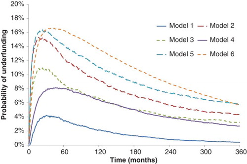
Fig. 3. This graph presents the probability that the scheme will be underfunded at time t; Prob(z_t<0). For Models 1–3, the results are as reported in Figure 1. For Models 4–6, it is assumed that asset returns are generated by a four-state Markov regime switching model. In Model 4, the discount rate is fixed at its current level. In Model 5, the discount rate follows a one-state O–U process that is independent of the portfolio return. Model 6 allows for the correlation between the discount rate and the portfolio return process within a Markov switching environment.

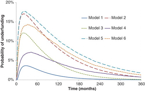
The difference between Models 4, 5 and 6 is in the treatment of the discount rate process. For comparison with Model 1, in Model 4 it is assumed that r_ft=r_f0 for all t. For comparison with Model 2, in Model 5 values of x_t are drawn at random and independently from the portfolio return from a normal distribution with mean a and variance . Therefore, although Model 5 includes Markov switching for the asset returns process, discount rates are driven as if there were only one state in the economy. From x_t, values of the discount rate are constructed iteratively by . In Model 6, the variable x_t is estimated as part of the Markov switching process and therefore its mean and variance are both state dependent, as is its correlation with the portfolio returns process. We use the standard Cholesky decomposition approach to construct correlated random variables r_pt, x_t at each time t within each simulation to capture the properties of the underlying state at that time.

The comparison of results of Models 4–6 are similar to those of Models 1–3. Assuming that the discount rate is constant leads to a substantial underestimation of the solvency risk, while assuming that the interest rate process is independent of the asset returns process leads to an overestimate of the risk because asset returns and the discount rate are negatively correlated.

By incorporating Markov switching, three new features emerge. First, the impact of introducing leptokurtosis into the asset returns process noticeably increases the assessed funding risk in all cases, but the impact is less dramatic than allowing for stochasticity in the discount rate. This is consistent with the summary statistics presented in the introduction to this paper as most of the volatility comes from changes in the calculated present value of liabilities rather than asset values. Second, in Models 4–6, the maximal probability of fund risk, at months 43, 29 and 33, respectively, occurs approximately one year later than in Models 1–3 (months 28, 21 and 21, respectively). Finally, the funding risk decays much more slowly under Models 4–6 than under Models 1–3. The at 30 years is under 1% of the maximal risk for Models 1 and 3 and approximately 4% for Model 2. By contrast, it is almost 9% for Models 4 and 6 and over 11% for Model 5. At longer horizons, the estimated risks from Model 6 are greater than those from Model 2. In addition to revealing the probability that z_t<0, the simulations also present broader statistical information about this variable. Table 4 presents summary statistics for z_t at horizons of one and five years for the four models with stochastic interest rates.

Table 4.  Summary statistics for the funding ratio, z_t.

	Mean	Median	Lower 2.5%	Upper 2.5%
		One-year horizon
Model 2	0.259	0.237	−0.188	0.834
Model 3	0.250	0.238	−0.127	0.699
Model 5	0.252	0.228	−0.197	0.843
Model 6	0.231	0.217	−0.141	0.680
		Five-year horizon
Model 2	0.762	0.636	−0.343	2.638
Model 3	0.723	0.645	−0.227	2.094
Model 5	0.741	0.595	−0.386	2.771
Model 6	0.610	0.500	−0.285	2.119

Notes: This table presents summary statistics for z_t, the funding ratio of the illustrative pension portfolio. Results are presented for all models with a stochastic interest rate and at time horizons of one and five years.

Again, the effects of more accurately modelling the underlying dynamics are dramatic. Despite starting with an initial funding surplus of , the most sophisticated model predicts that the lower 2.5% of funds will be more than 14% in deficit after 12 months and double that after 5 years. This again emphasises not only the probability of falling into a funding shortfall, but also, in a VaR sense, how severe such a fall might be.

5. Extensions

In this section, we briefly consider four extensions to our main models: applying the Markov framework to more realistic liability models, an examination of how well the different models performed in explaining the observed change in aggregate DB pension plan funding during the credit crisis, the impact of parameter uncertainty, and reduced-form model estimation with fewer asset classes and states of the world.

5.1. Comparison with results using a more refined liability model

As noted in Section 2, our objective in this paper is to understand the impact of different econometric choices on assessed future funding risk. We have therefore in the main focused on a highly stylised form for the expected future liabilities of the modelled DB scheme. In practice, though, it would be necessary to apply the models to considerably more complex future cash flow structures. To test the robustness of our findings to this issue, we passed our Markov switching calibrations for Models 1 and 4 to Nematrian Limited, a professional consultancy firm with expertise in actuarial pension fund analysis. It applied these calibrations to its own model of final salary-type pension schemes. Where use of this more sophisticated liability model provides greater insight is in understanding the impact of features of the liability profile that are not well catered for in the highly stylised model used earlier. For example, the more realistic liability model used here includes amortisation of surpluses and deficits via assumed changes to sponsor contribution rates. In the limiting case where surpluses and deficits are amortised infinitely quickly then variability in the asset–liability ratio disappears (to be replaced by variability in the sponsor contribution rate), highlighting that in practice will be sensitive to funding policy as well as asset returns.

This model includes a range of active, deferred and pensioner members. The scheme is closed to new entrants but open to new accrual for active members. It incorporates some decrement assumptions between the different categories together with some mortality assumptions. Active members’ benefits are assumed to increase in line with salary inflation at 5% per annum, while deferred members’ and pensioners’ benefits are assumed to increase in line with price inflation at 3% per annum in deferment and in payment. The scheme is assumed to be initially 100% funded on an ongoing funding basis with the split of liabilities being actives 12%, deferreds 33% and pensioners 55%. About 20% of any surpluses or deficits arising were assumed to be amortised each year by way of adjustment to contributions in that year. The likelihood of sponsor default was assumed to be zero throughout the projection period. In our online supplementary material, we provide a spreadsheet that illustrates the Nematrian model and will allow the reader to vary the assumptions contained therein. Figure 4 presents results for Prob(z_t<0) based on 1000 simulations. Consistent with our earlier results, a noticeably higher probability of being underfunded arises with Model 4, which includes Markov switching, than with Model 1 throughout the projection period.

Fig. 4. This graph presents the probability that the scheme will be underfunded at time t; Prob(z_t<0). This is based on the scheme of liabilities from the proprietary model of Nematrian Limited. Results are based on 1000 simulations.

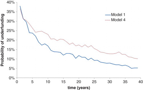
This analysis suggests that broadly similar overall conclusions can also be drawn if we had adopted a more realistic liability model than is presented in the earlier sections of this paper. The precise impact on funding risk at a given time does, though, depend heavily on the shape of the liabilities and also what assumptions are made regarding how surpluses and deficits are amortised by adjustments to future contribution rates.

5.2. The credit crisis

A macroprudential regulator would not primarily be interested in one individual scheme but instead would wish to focus on the aggregate systematic funding risk across the sector. This would require her to look at heterogeneity across funds. To consider that issue here, we look at variations in initial funding positions, z₀, but continue to assume that asset allocations are constant across schemes. Within each simulation, the value of z₀ is now drawn at random from a distribution. This matches well three features of the PPF 7800 index for June 2007, the final month before the aggregate funding positions of DB schemes began to deteriorate. First, the mean value of 24.1% matches the average funding position in that month. Second, the cumulative distribution function value for z₀=0 under this distribution is 12.2%. This matches the proportion of liabilities that lay within funds that were in deficit at the end of this month. Third, from the properties of a truncated normal distribution, the theoretical average value of z₀ for funds in surplus (deficit) is +28.9% and −10.2%. These are very close to the reported values of +28.9% and −10.6%, respectively.

For all six models, we then estimate by simulation for horizons up to five years the proportion of liabilities that are predicted to lie within funds that are in deficit. For Models 4–6, we place an initial probability 1 on the current state being the crash state (State 4 for Models 4 and 5, and State 1 for Model 6) to reflect the arrival of the credit crisis. Results are reported in Figure 5.

Fig. 5. This graph presents the probability that the scheme will be underfunded at time t; Prob(z_t<0). The initial level of funding is set at random across simulations through the distribution z₀∼ N(24.1%, 20.7%). This broadly reflects the cross-sectional spread of pension fund solvency before the credit crisis hit. For Models 4–6, the economy is initially set to the crash state with probability 1.

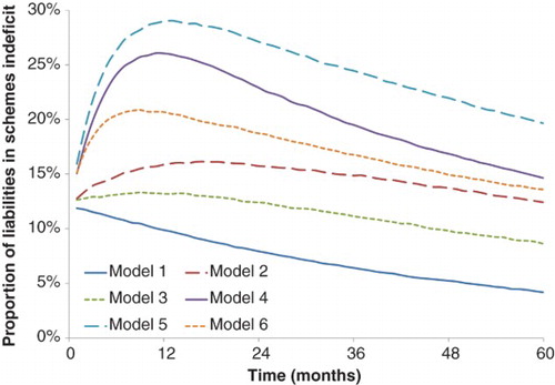
Under Models 1 and 3, the funding position is expected to improve over the coming 60 months, while Model 2 predicts a small worsening before a gradual improvement. By contrast, both Models 4 and 5 point towards a more than doubling of underfunding over the next 12 months. For Model 5, the proportion of liabilities within underfunded schemes rises from the initial value of 12.2% to 29.0% at 13 months, a 138% increase. Model 6 also predicts high levels of underfunding in one year, but less so than Model 4 or 5. The principal reason for this is that State 1 in Model 6 is more transitory (50% probability of persistence) than State 4 in Models 4 and 5 (86% probability of persistence). Therefore, setting the initial state to the crash state has less impact on Model 6 than on either Model 4 or 5.⁹

From this we can conclude that, while still underestimating the observed level of underfunding that followed the credit crisis, the four-state models would have given the macroprudential regulator materially better guidance than the single-state model.

5.3. Parameter uncertainty

Throughout this analysis we have assumed that all parameter values are known with certainty. We now extend the analysis to allow for estimation error. For Model 3, we incorporate parameter uncertainty in m, a, b and ρ but assume that the variances of the asset return and interest rate processes (σ² and , respectively) are known without error. This is because, in an i.i.n.d. world, the variance can be estimated to any required level of precision by increasing the sample frequency of the data. In this case, it is well known that , where is the number of data points in the observed sample. It is also well know that â and bˆ, when estimated from ordinary least-squares regression, are multivariately normally distributed with where is the sample average of r_ft and . To incorporate uncertainty into ρ, we employ the transformation of Fisher (1921), who noted that if we define then, to good approximation, . Models 1 and 2 are nested within Model 3.

For the four-state models, the MSVAR output does not provide any information on parameter uncertainty. Therefore, we take an alternate approach. Throughout we assume that both the variances and the transition probability matrix (and hence the ergodic probabilities) are estimated without error. In Model 4, we estimate the uncertainty in m_s through the standard error , where , which can be broadly interpreted as the number of observations during the sample period when the market was in state s. In Model 5, we also include the interest rate stochasticity by combining the uncertainty components of Models 4 and 2. In Model 6, we allow for parameter uncertainty in m_s, a_s and the state-dependent correlation, ρ_s, between e_pt and e_ft. For the a_s component, we again use the simple standard error, this time based on the state-dependent volatility of the interest rate process . Uncertainty in ρ_s is again captured through the Fisher transformation given above, with replaced by ς_s, ρˆ_s for each state s.

Figure 6 presents the results, constructed through 250,000 simulations. For model 3, we discard all simulations with b<0 to prevent mean-averting interest rate processes.

Fig. 6. This graph presents the probability that the scheme will be underfunded at time t; Prob(z_t<0). This extends Figure 3 by allowing for parameter uncertainty.

For Models 1, 4, 5 and 6, parameter uncertainty raises the underfunding risk at all horizons. The most important effect is that the risk persists into the much more distant future in all models, while the shorter term effects are of less practical significance. In Models 2 and 3, at near time horizons, the risk of insolvency gets lower. The reason for this is that, under the baseline parameterisations, and the value of bˆ is low, implying very slow mean reversion. However, in the simulations, b varies. By imposing the restriction that b>0, to avoid mean-averting processes, we allow the value of b to get greater, but there is only limited room for movement on the downside. Therefore, on average, there is stronger mean reversion in the parameter uncertainty case, resulting in the interest rate rising more quickly with parameter uncertainty. These effects lower the stochasticity in and reduce the expected present value of liabilities, thus dampening the risk of future underfunding. As might be expected, though, for longer horizons parameter uncertainty significantly increases the risk of insolvency for all models that we consider.

We have also, in unreported results, re-calibrated Models 1–5 using data for the more restricted period January 1991 to December 2010.¹⁰ The overall pattern of underfunding risk is broadly similar to the results discussed above. The main difference in this case is that the AR(1) interest rate model mean reverts more quickly, , giving a half-life of approximately three and a half years. As a consequence there is less stochasticity in , leading to greater similarities between Models 2 and 3 with Model 1. The maximal probability of being in deficit is 4.9% under Model 1, 9.1% under Model 2 and 5.5% under Model 3. The greatest probability of default arises in this case under Model 5, 10.5% at 28 months.

5.4. Reduced-form models

The fact that the MSVAR estimation did not converge for Model 6 over the 1991–2010 period clearly illustrates that it may sometimes be necessary for practitioners to work with more reduced-form versions of these models. In this subsection, we consider only three asset classes and either two or three states. This significantly lowers the computational burden on the Markov estimation process.¹¹

The three asset classes that we now consider are world equities, nominal gilts and index-linked gilts (ILGs). The UK nominal Treasury bond data are as described in Section 2.1; we use the MSCI world index, sterling denominated, for equities and calculate returns to ILGs from a total returns index reported in the British Government Securities Database maintained by Professor Andrew Cairns at Heriot-Watt University. The estimation period is now November 1998 to December 2010, reflecting the recent availability of an ILG total returns index. We use the same O–U residuals for the risk-free rate as for the 1991–2010 period. The weightings that we use now place somewhat greater weight on fixed income than in earlier calibrations: 40% in world equity and 30% each in nominal bonds and ILGs. Because of the lower average returns in this estimation period, we lower the fixed inflation rate . In total, there are four new sets of calibration results and simulations: S=2,3 and estimates that include/exclude the risk-free rate process within each regime (Models 4 and 5/Model 6). We report summary statistics for these calibrations in Table 5.

Table 5.  Summary statistics for the reduced-form model.

	Mean	Standard deviation	π	Corr(rp, xt)	Correl
		Two state: Models 4 and 5
State 1	−0.66%	4.37%	5.2%	n/a	66.9%
State 2	0.40%	1.69%	94.8%	n/a	−27.0%
		Two state: Model 6
State 1	−1.40%	4.68%	3.3%	−97.5%	75.4%
State 2	0.39%	1.76%	96.7%	−17.2%	−23.0%
		Three state: Models 4 and 5
State 1	−3.51%	1.92%	3.4%	n/a	59.5%
State 2	0.36%	1.68%	93.8%	n/a	−26.5%
State 3	4.37%	1.54%	2.8%	n/a	76.9%
		Three state: Model 6
State 1	−1.67%	2.21%	10.8%	−10.8%	27.7%
State 2	0.44%	1.56%	71.7%	−1.5%	−37.9%
State 3	2.26%	1.55%	17.5%	−63.2%	18.8%

Notes: This table is similar to Tables 2 and 3, but presents summary statistics for the Markov switching environment with either two or three states and three asset classes. This is for the period 1998–2010 and the assets are world equities, nominal gilts and ILGs. The ‘Models 4 and 5’ (‘Model 6’) calibrations exclude (include) x_t which is a measure of the change in risk-free rate and that is formally defined in the body of the text. ‘Correl’ is the correlation between world equity and nominal gilt returns.

The Akaike information criterion and other similar measures prefer the three-state calibrations for both Models 4 and 5 and Model 6. In addition, the ‘crash’ state is much more clearly revealed in the three-state calibration in terms of expected return, although less so in volatility. For S=3, Models 4 and 5, the average annualised return in State 1 is below −40%. Therefore, in Figure 7, we present the equivalent of Figures 3 and 6 for these calibration, with each line representing the probability that a fund that is currently overfunded by 15% falls into deficit at some future time; .

Fig. 7. This graph presents the probability that the scheme will be underfunded at time t; Prob(z_t<0). This extends Figures 3 and 6 by reducing the number of asset classes to three (world equities, nominal gilts and ILGs), the number of state S=3 and changing the estimation period to 1998–2010.

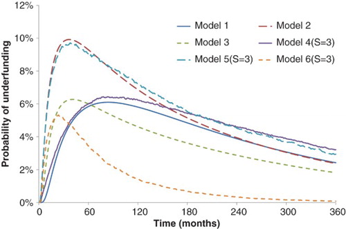
As before, Models 2 and 5, which includes independent stochasticity in the discount rate, indicate much higher risk than a fixed cost of capital model (Models 1 and 4). Including the correlation between asset returns and discount rates (Models 3 and 6) again reduces the perceived maximum risk. These now become similar to the maximum risk levels estimated by the simplest models, which contrasts with earlier results, although the greatest risk occurs much sooner under the more complex calibrations. By comparing Models 4–6 against Models 1–3 we continue to see the impact of allowing for Markov switching in the calibrations. For Models 4 and 5, the long-term underfunding risk is significantly increased by incorporating Markov switching, consistent with earlier sections of this paper. However, counter to previous results, the long-run estimated solvency risk is much lower under Model 6 than under Model 3. We also consider in Table 6 the impact of different asset allocation choices on funding risk. In Panel A, the proportion of equity varies, with the residual split equally between nominal bonds and ILGs, while in Panel B the proportion of equities is fixed at 40% and the residual split in different ways between the two Treasury securities. In each case, we present descriptive statistics for the per-period FRR, FRR_t, and also the probability that z_t<0. This table is based on Model 6, S=3 for a 60-month investment horizon.

Table 6.  Varying the asset allocation.

Weight	Weight	Weight	Mean	Std	Skew	Ex. Kurt.	Underfunding	Expected
equity (%)	gilts (%)	ILGs (%)	FRR (%)	FRR (%)	FRR	FRR	risk (%)	utility
Panel A: Variable equity weight
0	50	50	0.31	0.18	−0.27	0.18	0.42	−0.076
10	45	45	0.34	0.20	−0.22	0.11	0.39	−0.071
20	40	40	0.37	0.24	−0.17	0.11	0.81	−0.069
30	35	35	0.40	0.29	−0.12	0.13	1.87	−0.070
40	30	30	0.43	0.36	−0.09	0.13	3.47	−0.075
50	25	25	0.47	0.43	−0.07	0.10	5.43	−0.082
60	20	20	0.50	0.51	−0.05	0.14	7.43	−0.094
70	15	15	0.53	0.58	−0.03	0.11	9.42	−0.112
80	10	10	0.56	0.66	−0.02	0.10	11.30	−0.140
90	5	5	0.59	0.74	0.00	0.12	13.05	−0.180
100	0	0	0.63	0.82	0.00	0.11	14.37	−0.246
Panel B: Variable fixed income weight
40	0	60	0.45	0.39	−0.10	0.12	4.37	−0.078
40	6	54	0.44	0.38	−0.11	0.12	4.14	−0.077
40	12	48	0.44	0.38	−0.10	0.15	3.97	−0.076
40	18	42	0.44	0.37	−0.09	0.13	3.81	−0.075
40	24	36	0.44	0.37	−0.09	0.12	3.59	−0.075
40	30	30	0.43	0.36	−0.09	0.10	3.49	−0.074
40	36	24	0.43	0.36	−0.09	0.14	3.33	−0.074
40	42	18	0.43	0.35	−0.09	0.13	3.25	−0.074
40	48	12	0.43	0.35	−0.08	0.14	3.20	−0.074
40	54	6	0.42	0.35	−0.09	0.12	3.10	−0.074
40	60	0	0.42	0.34	−0.09	0.16	3.10	−0.074

Notes: In this table, we illustrate the impact of different asset allocations on scheme solvency risk. The investment horizon is five years, t=60 months, and is based on the 1998–2010, three-asset class, three-state Model 6 described in Section 5.4. Columns 1–3 give the portfolio weights, columns 4–7 present the first four moments of the per-period FRR, FRR_t, and column 8 presents the probability that z_t<0. Column 9 gives the expected utility when CRRA preferences are stated on the funding ratio and the coefficient of relative risk aversion is 5.

As the proportion of equity increases, so the expected FRR, its volatility and the probability of becoming underfunded all increase. This illustrates the standard risk-return dilemma faced by investment managers. With equity fixed at 40%, the underfunding risk decreases slowly as we switch out of ILGs and into nominal Treasury bonds. This is primarily because the standard deviation of the funding ratio reduces slightly with a higher proportion of gilts as these are a marginally better hedging asset for world equities. To consider what might be the optimal portfolio, we follow Hoevenaars et al. (2008) by specifying constant relative risk aversion (CRRA) preferences on the funding ratio, , where γ is the measure of risk aversion which we set equal to five. The expected utility is presented in the final column of Table 6 for each portfolio. This indicates that the optimal weight in equity is around 20%. When the equity weight is fixed at 40%, expected utility is largely insensitive to asset allocation within the fixed income portion of the portfolio, but the optimal mix appears to be approximately 90% gilts to 10% ILGs.

6. Conclusion

In 2008, the global financial crisis resulted in significant falls in asset values and dramatically reduced interest rates. For pension funds, this presented the perfect storm. Asset values were depressed, while the discount rate for estimating the present value of the liabilities was pushed lower, resulting in inflated liabilities. Jointly, the effect was to leave huge deficits on the balance sheet of DB pension funds. As a result, to better estimate future solvency scenarios it is critical that both asset returns and discount rates are modelled jointly.

To undertake this analysis we use Markov regime switching models. The modelling choice seems appropriate given its widespread use in both academic and practitioner work. Moreover, this type of modelling addresses some of the key issues raised by the Actuarial Profession BSM Working Party as it captures extreme market movements. Markov regime switching models can capture rare, but extreme market events, time-varying asset return volatility and the fat-tailed nature of stock returns.

Our results show the importance of estimating a stochastic discount rate process that is allowed to vary with asset returns. If interest rates remain constant through time, then both the standard one-state model and the multi-state Markov regime switching model significantly underestimate the likelihood of future pension plan deficits compared to an independently stochastic interest rate process. For both the one-state and multi-state models, when interest rate changes vary with asset returns, the estimated proportion of underfunded pension plans is higher than in the case with fixed discount rates (except in our final calibration) but lower than when interest rates move independently from asset returns. In our main calibration with correlated interest rates and asset returns, incorporating multiple states predicts between approximately 2.5% and 4.5% more underfunded schemes than the one-state model and this number is persistent through time.

These results have a number of pension fund management and policy implications. From a pension management perspective, the advice given to trustees and sponsors must be carefully explained. The presentation of one result, or one type of result (i.e. a fixed discount rate), does not present an accurate picture for effective decision-making. In particular, a much broader and clearer discussion about potential outcomes would allow for more effective decision-making around issues such as short-term and long-term funding plans, potential risk management strategies and asset allocation decisions.

Understanding the potential impact of these different outcomes in both the short and long run has huge implications for macro-prudential pension regulation. For example, if our models were re-calibrated to incorporate a sustained period of low asset returns, then the percentage of funds that are likely to have deficits would increase at our furthest-out projections. Consequently, a much richer data set of future pension outcomes can be estimated and better decisions made in terms of pension funding at a macro level. Moreover, from the perspective of The UK Pensions Regulator scheme, specific sensitivities to potential future outcomes could be considered. The identification of ‘at-risk’ schemes may become better, while for the Pension Protection Fund a richer set of scenarios could be projected that may help with the identification of potential funding pressures in the future.

Acknowledgements

The authors gratefully acknowledge financial support from the Rotman International Centre for Pension Management (ICPM) at the University of Toronto and from the Actuarial Profession in the UK. We would also like to thank the anonymous referees, conference participants at the October 2011 Discussion Forum co-hosted by ICPM and World Bank Treasury in Washington DC, the Fifth International Conference in Mathematical and Statistical Methods for Actuarial Sciences and Finance, Venice 2012, and participants at the May 2012 Actuarial Profession Sessional Meeting in Leeds, as well as seminar participants from the University of Leeds, the University of Bradford and the University of Sheffield for their useful and insightful comments as this work has developed. The views expressed in this paper reflect those of the authors and not of the ICPM or the Actuarial Profession. All errors remain our own.

Notes

1. The Pension Protection Fund PPF 7800 index covers 6150 UK pension schemes. There were three actuarial changes in index construction technique during this period.

2. For evidence of the reduction in DB scheme membership in the UK, see http://www.ons.gov.uk/ons/dcp29904_272194.pdf. For an example of changes in DB terms, see http://www.uss.co.uk/Members%20Annual%20Reports/Proposed%20Changes%20(Act%20MAR)%20WEB.pdf. Both websites accessed 3 July 2013.

3. While this is a common assumption in both industry and academia, it is not uncontroversial. For example, there is an extensive literature that argues that average historic returns to equity substantially overestimate the current ex ante equity premium (Freeman 2011).

4. According to the 2013 PPF Purple Book, 35.1% of UK pension funds were in equity, 44.8% were in bonds and 20.2% were in other assets, including hedge funds, property, cash and insurance products. Of the equity proportion, 31.0% was UK based, 61.3% international equity and 7.7% unquoted. The bond portfolio comprises a mix of vanilla Treasuries, corporate bonds and index-linked bonds. The weights that we use here broadly reflect this balance while limiting the number of asset classes to five. It would be straightforward to adjust our techniques to allow for time variation in asset allocation but this is not undertaken here for reasons of parsimony.

5. While we do not necessarily advocate risk-free discounting of pension liabilities, the choice of this rate is essentially consistent with section 179 of the Pension Protection Act. Again, the methods that we use are broadly insensitive to the choice of yield that is used for discounting purposes.

6. This is the main justification for estimating the Markov switching process at the individual asset class level rather than the portfolio level. Had we estimated switching for portfolio returns alone, then it would not be possible to dynamically change the weightings within future simulations should a fund manager wish to do so.

7. Approximate sample standard deviations for the mean, skewness and kurtosis statistics were calculated as and , respectively, where n=491 is the number of observations and σ the estimated volatility of the data. Approximate 95% confidence intervals for each statistic are then calculated as the sample mean ±1.96 standard deviations. The standard deviation confidence interval is calculated from the chi-squared statistic with 490 degrees of freedom.

8. In unreported results, we also run simulations for Models 1–3 to check the sensitivity of our results to the method of their derivation. The simulation results are, in all cases, highly similar to those reported in Figure 1. An issue also arises as to whether to start the simulations according to the ergodic probabilities or the estimated smoothed probabilities in December 2010 that are an output from the Markov estimation process. The former is more suitable for our purposes as we are comparing modelling choices and are therefore reporting unconditional estimates. For a fund manager assessing his or her own fund risk in December 2010, it would be more appropriate to use the smoothed probability estimates for that date.

9. When we set the initial state to a non-crash state (State 2 for Models 4 and 5 and State 3 for Model 6) then, as would appear realistic, these models forecast decreasing funding risk over the next five years (although, as with Model 2, there is a small increase in risk for Model 5 over approximately one year before the decline begins). Conditioning the four-state model, therefore, does not always lead to forecasts of higher future funding risk.

10. Model 6 has 120 parameters to estimate and we were unable to make the MSVAR code converge in this case when using only 240 data points. Further details on all these simulations are available on request from the authors.

11. We thank an anonymous referee for suggesting that we run these more reduced-form models. We have also tried to calibrate an S=4 version of this model but because of the low number of observations, the MSVAR estimates do not converge in this case.

References

- Ang, A., and G. Bekaert. 2002. “International Asset Allocation with Regime Shifts.” Review of Financial Studies 15 (4): 1137–1187. doi: 10.1093/rfs/15.4.1137
- Ang, A., and A. Timmermann. 2011. “Regime Changes and Financial Markets.” Netspar Discussion Paper #DP 06/2011-068.
- Billio, M., and L. Pelizzon. 2000. “Value-at-Risk: A Multivariate Switching Regime Approach.” Journal of Empirical Finance 7 (5): 531–554. doi: 10.1016/S0927-5398(00)00022-0
- Boyle, P. P., and T. Draviam. 2007. “Pricing Exotic Options Under Regime Switching.” Insurance: Mathematics and Economics 40 (2): 267–282.
- Chollette, L., A. Heinen, and A. Valdesogo. 2009. “Modeling International Financial Returns with a Multivariate Regime-Switching Copula.” Journal of Financial Econometrics 7 (4): 437–480. doi: 10.1093/jjfinec/nbp014
- Cochrane, J. H. 2011. “Presidential Address: Discount Rates.” Journal of Finance 66 (4): 1047–1108. doi: 10.1111/j.1540-6261.2011.01671.x
- Dueker, M., and C. J. Neeley. 2007. “Can Markov Switching Models Predict Excess Foreign Exchange Returns?” Journal of Banking and Finance 31 (2): 279–296. doi: 10.1016/j.jbankfin.2006.03.002
- D. W. P. 2013. Pensions and Growth; Whether to Smooth Assets and Liabilities in Scheme Funding Valuations: A Call for Evidence. London: The Department of Work and Pensions.
- Elliott, R. J., and H. Miao. 2009. “VaR and Expected Shortfall: A Non-Normal Regime Switching Framework.” Quantitative Finance 9 (6): 747–755. doi: 10.1080/14697680902849320
- Elliott, R. J., and T. K. Siu. 2009. “On Markov-Modulated Exponential-Affine Bond Price Formulae.” Applied Mathematical Finance 16 (1): 1–15. doi: 10.1080/13504860802015744
- Embrechts, P., S. I. Resnick, and G. Samorodnitsky. 1999. “Extreme Value Theory as a Risk Management Tool.” North American Actuarial Journal 3 (2): 30–41. doi: 10.1080/10920277.1999.10595797
- Ferstl, R., and A. Weissensteiner. 2011. “Asset-Liability Management Under Time-Varying Investment Opportunities.” Journal of Banking and Finance 35 (1): 182–192. doi: 10.1016/j.jbankfin.2010.07.028
- Fisher, R. A. 1921. “On the ‘Probable Error’ of a Coefficient of Correlation Deduced from a Small Sample.” Metron 1: 3–32.
- Frankland, R., A. D. Smith, T. Wilkins, E. Varnell, A. Holtham, E. Biffis, S. Eshun, and D. Dullaway. 2008. “Modelling Extreme Market Events: A Report of the Benchmarking Stochastic Models Working Party.” Institute of Actuaries and Faculty of Actuaries.
- Fraudendorfer, K., U. Jackoby, and A. Schwendener. 2007. “Regime Switching Based Portfolio Selection for Pension Funds.” Journal of Banking and Finance 31 (8): 2265–2280. doi: 10.1016/j.jbankfin.2007.02.003
- Freeman, M. C. 2011. “The Time-Varying Equity Premium and the S&P500 in the Twentieth Century.” Journal of Financial Research 34 (2): 179–215. doi: 10.1111/j.1475-6803.2011.01288.x
- Guidolin, M., and A. Timmerman. 2006a. “An Econometric Model of Nonlinear Dynamics in the Joint Distribution of Stock and Bond Returns.” Journal of Applied Econometrics 21 (1): 1–22. doi: 10.1002/jae.824
- Guidolin, M., and A. Timmerman. 2006b. “Term Structure of Risk Under Alternative Econometric Specifications.” Journal of Econometrics 131 (1–2): 285–308. doi: 10.1016/j.jeconom.2005.01.033
- Guidolin, M., and A. Timmerman. 2007. “Asset Allocation Under Multivariate Regime Switching.” Journal of Economic Dynamics and Control 31 (11): 3503–3544. doi: 10.1016/j.jedc.2006.12.004
- Guidolin, M., and A. Timmerman. 2008. “International Asset Allocation Under Regime Switching, Skew, and Kurtosis Preferences.” Review of Financial Studies 21 (2): 889–935. doi: 10.1093/rfs/hhn006
- Hamilton, J. D. 1989. “A New Approach to the Economic Analysis of Non-Stationary Time-Series and the Business Cycle.” Econometrica 57 (2): 357–3840. doi: 10.2307/1912559
- Hamilton, J. D., and R. Susmel. 1994. “Autoregressive Conditional Heteroskedasticity and Changes in Regime.” Journal of Econometrics 64 (1–2): 307–333. doi: 10.1016/0304-4076(94)90067-1
- Hoevenaars, R. P. M. M., R. D. J. Molenaar, P. C. Schotman, T. B. M. Steenkamp. 2008. “Strategic Asset Allocation with Liabilities: Beyond Stocks and Bonds.” Journal of Economic Dynamics and Control 32 (9): 2939–2970. doi: 10.1016/j.jedc.2007.11.003
- Josa-Fombellida, R., and J. P. Roncón-Zapatero. 2011. “Optimal Asset Allocation for Aggregated Defined Benefit Pension Funds with Stochastic Interest Rates.” European Journal of Operational Research 201 (1): 211–221. doi: 10.1016/j.ejor.2009.02.021
- Kawata, R., and M. Kijima. 2007. “Value-at-Risk in a Market Subject to Regime Switching.” Quantitative Finance 7 (6): 609–619. doi: 10.1080/14697680601161795
- Kemp, M. 2011. Extreme Events: Robust Portfolio Construction in the Presence of Fat Tails. Chichester: John Wiley.
- Lam, P. S. 1990. “The Hamilton Model with a General Autoregressive Component.” Journal of Monetary Economics 26 (3): 409–432. doi: 10.1016/0304-3932(90)90005-O
- Leibowitz, M. L., S. Kogelman, and L. N. Bader. 1994. “Funding Ratio Returns.” Journal of Portfolio Management 21 (1): 39–47. doi: 10.3905/jpm.1994.409495
- Longin, F. M. 1999. “Optimal Margin Level in Futures Markets: Extreme Price Movements.” Journal of Future Markets 19 (2): 127–152. doi: 10.1002/(SICI)1096-9934(199904)19:2<127::AID-FUT1>3.0.CO;2-M
- Mercer/ICAEW. 2012. “Living with Defined Benefit Pension Risk: A Survey of Major Employers.” Mercer and the Institute of Chartered Accountants in England and Wales.
- Okimoto, T. 2008. “New Evidence of Asymmetric Dependence Structure in International Equity Markets.” Journal of Financial and Quantitative Analysis 43 (3): 787–815. doi: 10.1017/S0022109000004294
- Psaradakis, Z., M. O. Ravn, and M. Sola. 2005. “Markov Switching Causality and the Money-Output Relationship.” Journal of Applied Econometrics 20 (5): 665–683. doi: 10.1002/jae.819
- Psaradakis, Z., M. Sola, and F. Spagnolo. 2004. “On Markov Error-Correction Models, with an Application to Stock Prices and Dividends.” Journal of Applied Econometrics 19 (1): 69–88. doi: 10.1002/jae.729
- Raymond, J. E., and R. W. Rich. 1997. “Oil and the Macroeconomy: A Markov State-Switching Approach.” Journal of Money, Credit and Banking 29 (2): 193–213. doi: 10.2307/2953675
- Sharp, W. F., and L. G. Tint. 1990. “Liabilities – A New Approach.” Journal of Portfolio Management 16 (2): 5–10. doi: 10.3905/jpm.1990.409248
- Shen, Y., and T. K. Siu. 2012. “Asset Allocation Under Stochastic Interest Rate with Regime Switching.” Economic Modelling 29 (4): 1126–1136. doi: 10.1016/j.econmod.2012.03.024
- Storer, P. A., and M. Van Audenrode. 1995. “Unemployment Insurance Take-Up Rates in Canada: Facts, Determinants and Implications.” Canadian Journal of Economics 28 (4a): 822–835. doi: 10.2307/135933
- Taamouti, A. 2009. “Analytical Value-at-Risk and Expected Shortfall Under Regime-Switching.” Finance Research Letters 6 (3): 138–151. doi: 10.1016/j.frl.2009.03.004
- Vaşicek, O. 1977. “An Equilibrium Characterisation of the Term Structure.” Journal of Financial Economics 5 (2): 177–188. doi: 10.1016/0304-405X(77)90016-2
- Weitzman, M. 2001. “Gamma Discounting.” American Economic Review 91 (1): 260–271. doi: 10.1257/aer.91.1.260
- Zhou, X. Y., and G. Yin. 2003. “Markowitz's Mean-Variance Portfolio Selection with Regime Switching: A Continuous-Time Model.” SIAM Journal on Control and Optimization 42 (4): 1466–1482. doi: 10.1137/S0363012902405583