Stock market contagion in Central and Eastern Europe: unexpected volatility and extreme co-exceedance

†The Online Appendix is available at http://ies.fsv.cuni.cz/en/staff/horvath.

Abstract

We examine whether there is contagion from the US stock market to six Central and Eastern European stock markets. We use a novel measure of contagion that examines whether volatility shocks in the US stock market coupled with negative returns are followed by higher co-exceedance between US and emerging stock markets. Using our approach and controlling for a set of market-related variables, we show that during the period from 1998 to 2014, financial contagion occurred, that is, unexpected negative events in the US market are followed by higher co-exceedance between US and Central and Eastern European stock markets. Even though contagion is stronger during the financial crisis, it also occurs in tranquil times.

Keywords:

• Contagion
• co-exceedance
• volatility
• stock markets

JEL Classifications:

• G01
• G14
• G15

1. Introduction

The global financial crisis was largely triggered by financial imbalances in the US economy that consequently spread around the world. The financial imbalances in developed countries significantly affected economic activity in many emerging economies, including those in Central and Eastern Europe (CEE), where GDP growth has fallen by double-digit numbers in some countries during the crisis. Although the overall evidence is somewhat mixed, several studies suggest that financial contagion has taken place in emerging economies in the past. Bae, Karolyi, and Stulz (2003) and Bekaert, Harvey, and Ng (2005) find evidence for contagion among Latin American countries and in Asia, respectively. This stream of literature focuses on examining the existence of financial contagion in emerging economies, especially during periods when emerging economies suffered from various forms of financial imbalances or even financial crises. As a result, it is not surprising that researchers find evidence of financial contagion under such circumstances.

Although existing studies often differ in their specific use and definition of the term financial contagion, most definitions share two attributes: (1) contagion is a negative event and (2) associated with increased co-movement between markets. Our use of the term financial contagion is most closely related to Bae, Karolyi, and Stulz (2003), as we consider contagion to be the joint occurrence of extreme return co-exceedances between two financial markets following an increase in unexpected volatility in one of the markets in the case that this stock market is plummeting.

However, to the best of our knowledge, evidence is lacking on whether financial contagion also occurs in emerging economies in times, when developed countries suffer from financial imbalances but the financial sectors in the emerging economies of interest remain largely stable. This is what largely occurred during the current global financial crisis, which began in the summer of 2007. While financial markets in the US and Western Europe had to obtain large financial injections from their governments, the financial sectors (dominated by banks) in Central European countries such as the Czech Republic, Slovakia and Poland remained largely stable and received no government support.¹

In addition, there is an extensive stream of literature examining stock market linkages between Central and Eastern European countries vis-à-vis Western Europe (see Wang and Moore 2008; Syllignakis and Kouretas 2011, among many others). Nevertheless, these studies largely focus on correlations and do not examine contagion, that is, correlations going beyond what would be implied by the fundamentals (Forbes and Rigobon 2002; Bekaert, Harvey, and Ng 2005, Bekaert et al. 2014). In this paper, we build upon the measure of financial contagion developed by Bae, Karolyi, and Stulz (2003), who define financial contagion as the joint occurrence of return co-exceedances between two financial markets.² We extend this measure and define financial contagion as ‘the joint occurrence of return co-exceedances between two financial markets following an increase in unexpected volatility in one of the markets in the case where that market experiences negative returns’.

The main contribution to the existing literature is the decomposition of the US stock market volatility into expected and unexpected components and examination of how unexpected volatility component increases the left-tail co-exceedance between stock markets. To our knowledge, this measure of financial contagion is novel and represents the main contribution of this paper. Within the quantile regression framework, we address specifically the left-tails of the distribution of return co-exceedances, that is, extreme market co-movements and their relationship to unexpected volatility component. Our notion of contagion is also conceptually in line with Bekaert, Harvey, and Ng (2005) and Bekaert et al. (2014), who define contagion as excessive co-movement over and above the predictions of a factor model, that is, what global equity market co-movements should be, based on existing fundamentals. Compared to Bekaert, Harvey, and Ng (2005) and Bekaert et al. (2014), our approach is different in that the return series is first filtered out of the effects of global factors and the resulting standardized residuals are used to compute co-exceedances, which are then linked to the unexpected part of the volatility.

We focus on six stock markets in the CEE. These markets represent a meaningful sample of the whole region of CEE markets in the European Union, which might be considered by international investors for diversification purposes. Our results provide evidence that an increase in the unexpected volatility in the US stock market, at the time US stock market falls markedly, leads to extreme negative joint co-movements between CEE and US stock markets. This result holds for a number of robustness checks such as using non-filtered measure of return co-movement, different time periods or different control variables in our quantile regression framework. As a consequence, our results indicate evidence of contagion from the US stock market to CEE markets. While we find that contagion is stronger during the financial crisis, it also occurs in good times.

The paper is organized as follows. Section 2 discusses the related literature. Section 3 presents the data. Section 4 provides our empirical methodology. The results are presented in Section 5. Concluding remarks are available in Section 6. An Appendix with additional results follows.

2. Related literature

2.1. Unexpected volatility and contagion

We define financial contagion as the occurrence of extreme return co-exceedances between two financial markets following an increase in unexpected volatility in one of the markets in the case where that stock market is plummeting. In line with the literature on contagion (e.g. King and Wadhwani 1990; Forbes 2012), a contagious event should be perceived by investors negatively. Therefore, contagion should be typically associated with bearish market conditions. Investors cannot be systematically surprised by fundamentals, that is, we expect that fundamentals are on average expected, and therefore, contagion should also be unanticipated. Otherwise, these events would have been already priced in. Even if investors are awaiting some news, expectations are already priced in, but the reality might be worse than expected. This negative and unexpected part of the news is what may cause contagion.

An important aspect of our definition of contagion is that we are not limited to identifying any crisis period a priori. A contagious event might be short-term (one day) event, somewhat negligible from a historical perspective, but still might induce excess co-movement between markets, unexplainable by fundamentals.

The existing literature examining contagion as an outcome of market over-reactions to unexpected events provides the rationale for our research. Studies examining the overconfidence of investors (e.g. Daniel, Hirschleifer, and Subrahmanyam 1998; Odean 1998, 1999; Barber and Odean 2001; Grinblatt and Keloharju 2009) suggest that after unexpected events, investors might react irrationally by ignoring fundamentals, thus propagating spillovers between international stock markets. More specifically, overconfidence can lead to excessive trading and volatility as investors over-react to new information (Daniel, Hirschleifer, and Subrahmanyam 1998; Barber and Odean 2001). Similar to the prospect theory of Kahneman and Tversky (1979), Hirschleifer (2001) argues that investors’ overconfidence follows from the fact that people in general tend to underestimate the probability of rare events. Investors are easily surprised by unforeseen contingencies, which lead to market over-reactions. The irrationality of investors is of course not the only possible explanation for increased co-movement during times of distress. Increased unexpected market volatility typically leads to increased observed volatility; thus, through volatility, our approach is related to the literature in which pricing is explained by market volatility.

For example, an increase in market volatility might increase the required return on equity, which leads to decline in stock prices, that is, the volatility feedback effect (e.g. Pindyck 1984; French, Schwert, and Stambaugh 1987; Wu 2001). Alternatively, volatility and returns act in a different causal order: negative returns increase financial leverage, which makes equities riskier; thus, equity prices become more volatile, that is, the leverage effect (e.g. Black 1976; Christie 1982; Bekaert and Wu 2000). Regardless of the underlying causes, an increase in unexpected market volatility signals mispricing. Such mispricing might be picked up by international investors, which leads to shock propagation across international equity markets (e.g. Kodres and Pritsker 2002; Boyer, Kumagi, and Yuan 2006).

2.2. Financial co-movements in the CEE region

The research on stock market integration (co-movements) in CEE countries is voluminous; however, contagion has rarely been investigated.

Syllignakis and Kouretas (2011) analyze co-movements between two developed markets (the US and Germany) and seven Central and Eastern European markets. They find that the estimated dynamic conditional correlations are systematically higher during the recent period of financial crisis in the US.

Samarakoon (2011) examines the spread of the financial crisis from the US stock market to 62 emerging and frontier stock markets, including those of the CEE region. His results suggest that what we observe is not contagion but rather a high sensitivity of emerging markets to events in the US market, that is, interdependence. According to his results, actual contagion is rare. Surprisingly, he finds contagion from emerging markets to the US market. However, this result might be a consequence of not considering non-synchronous trading effects.

Other studies apply some version of the multivariate GARCH model in an attempt to measure a ‘significant increase in cross-market linkages’ in line with the simplest and most utilized definition of contagion by Forbes and Rigobon (2002). Such studies include, inter alia, those of Cappiello et al. (2006), Savva and Aslanidis (2010) and Kenourgios and Samitas (2011). For most of the CEE countries, a significant increase in dynamic correlations has been confirmed during the recent financial crisis, thus indirectly implying the presence of contagion.

Correlation analysis is, however, only suitable to measure the contagion within the definition of Forbes and Rigobon (2002). In broader terms, ‘true’ contagion (when all fundamental channels are controlled for) is much more difficult to capture. Some attempts to explain dynamic conditional correlations among developed and CEE stock markets through fundamentals have been made (e.g. Wang and Moore 2008 or Büttner and Hayo 2011). However, cross-market linkages between the CEE region and developed markets appear to be driven by factors other than macroeconomic or financial fundamentals; perhaps they are driven by international investors and their herding behavior. The goal of our study is to bridge this gap and analyze the phenomenon of financial contagion in the CEE region in a more comprehensive way.

Compared to most existing studies, Bekaert et al. (2014) use industry-level stock market data to uncover how contagion spreads within countries and within similar industries. They find support for the ‘wake-up call’ hypothesis, that is, that the shocks in one market induce investors to re-valuate fundamentals in other markets, which is observed as the increased co-movement across markets (industries). Reboredo, Tiwari, and Albulescu (2015) examine time-varying dependence among several CEE markets (the Czech Republic, Hungary, Poland and Romania). Using dynamic copulas, they also find that this dependence intensified during the recent global financial crisis.

3. Data

We study contagion from the US stock market towards CEE stock markets. For US-based investors, CEE markets represent a geographically, economically and politically distinct class of investment opportunities. Our sample of CEE stock markets includes the following countries: Croatia, the Czech Republic, Estonia, Hungary, Poland and Romania. Using 1998–2011 data from the World Bank database (World Development Indicators) on Market Capitalization, among 18 CEE markets (excluding Russian Federation and including Balkan states) the six markets correspond to about 90% of the overall capitalization in the region (with Poland alone accruing for approximately 50–60%). We therefore consider the given sample to be representative of the CEE region. We choose these CEE countries because their stock markets are sufficiently capitalized, which is not the case in some other CEE countries such as Slovakia. The development of the CEE emerging stock markets is measured via daily continuous returns of the following market indices: CROBEX, PX, OMX Tallinn, BUX, WIG20 and BET.

We use data from 1 January 1998 to 31 December 2014. The sample covers the dotcom bubble, the subsequent steady growth of the US stock market, peak of the recent global financial crisis in 2008 and its consequences for the real economy of the CEE countries, the surge in oil prices, uncertainty over the US debt ceiling and the sovereign debt crisis in Europe, particularly including the uncertainty in the government bond market. Such a diverse sample should be sufficiently long to capture any contagious tendencies from the US stock market to the CEE stock markets. We use continuous returns of the S&P 500 stock market index to proxy the daily developments in the US stock market.

We estimate return co-exceedances from prices denominated in local currencies, as we do not want to blur the extent of market co-movements with fluctuations on the foreign exchange market (Mink 2015). However, we use daily returns on the foreign exchange market in the subsequent analysis as one of explanatory variables for co-exceedance. We use exchange rates between the US dollar and the corresponding local currency with one exception, for Estonia, where we use the exchange rate between the US dollar and the euro because before the adoption of the euro in 2011, the Estonian Kroon was fixed to the euro.

The fluctuations in the developed stock markets are captured using the daily continuous returns of the STOXX Global 1800 (excluding North America) index denominated in the US dollar . We make use of this index to account for common price-determining factors. When predicting US market volatility, we use the implied stock market volatility, the VIX, to account for the overall uncertainty of investors. We have also utilized a fundamentally different index to measure the uncertainty in the US economy: changes in the daily news-based Economic Policy Uncertainty Index (P_t) (Baker, Bloom, and Davis 2016). The index is based on the number of articles in over 1000 US newspapers about the economy. For a recent application, see Mensi et al. (2014), who use the policy index to explain returns on the BRICS stock markets.

Turbulent periods on stock markets may be accompanied by flight to quality, which drives the yield on low-risk bonds down. The recent period of ultra-low low-risk bond rates is by all standards unique. Decreases in low-risk bond yields decrease the required return, which might drive investors to emerging markets seeking new investment opportunities. Measuring such market conditions and tendencies is based on market yields on US Treasury securities at 20-year constant maturity .

We also use continuous daily returns from the Europe Brent Spot Price and the Gold spot price (at PM fix; ), both in US dollars, to control for short-term shocks which might be induced in these two commodity markets.

4. Methodology

Our test for contagion is performed within a quantile regression framework, where extreme left-tail co-movement between the US stock market and a given CEE stock market is explained via expected and unexpected market volatilities and a set of control variables. We therefore start by explaining the derivation of the co-movement variable (return co-exceedance) and the derivation of the expected and unexpected market volatility. We show in Section 4.1 how we compute return co-exceedances based on the standardized residuals from ARMAX(p, q)-EGARCHX(r, f) models. We present in Section 4.2 the specification for estimating expected and unexpected volatility components using range-based heterogeneous autoregressive (RB-HAR) model. Finally, in Section 4.3, we link together co-exceedances with decomposed volatility within the quantile regression approach.

4.1. Return co-exceedances

Our testing procedure is essentially based on the work of Baur and Schulze (2005), who modify the co-exceedance measure of Bae, Karolyi, and Stulz (2003) and analyze it using a quantile regression approach. Their modification allows us to measure the extent of excess market co-movement. To measure co-exceedances we use a formula similar to Baur and Schulze (2005): (1) where s_it and s_jt denote standardized residuals with zero mean and variance of 1 and subscripts i and j (i ≠ j) correspond to two examined markets. The local (or potentially infected) market is denoted as i and the potentially contagious market as j. In all of the regression specifications, the potentially contagious market is the US market, and the local market is one of the six stock markets, namely those in Croatia, the Czech Republic, Estonia, Hungary, Poland and Romania.

With daily data frequency, we must address the non-synchronicity of returns. We employ the fact that the US stock markets end their trading sessions last on a given calendar day t to our advantage and align the returns of the CEE markets at time t with the returns at t − 1 on the US market. This approach allows us to study the spread of contagion, that is, the direction of contagion from the US market to the other CEE stock markets.

We report the results where the return co-exceedances are based on the standardized residuals derived from an ARMAX(p, q)-EGARCHX(r, f) model. One might consider our filtering procedure of returns to be a factor model of returns (Forbes and Chin 2004), which assumes that market returns are a function of global factors (oil, gold prices), cross-country factors (foreign exchange returns and returns on other stock markets) and other market moving factors (US treasury bond yields). This way, we isolate shocks which originate in a given country and we are therefore in the domain of ‘pure/true contagion’³ instead of ‘monsoonal’ effects.⁴

For each series of returns r_t, t ∈ T we estimate an ARMAX (p, q) model: (2) where α_k, φ_i, θ_j and σ_t are model parameters. To account for the movements in the oil, foreign exchange, bond, gold and other developed equity stock markets (proxied by the STOXX 1800 index), we include the following returns in the mean equation: , , , and .

We model the evolution of via Nelson’s (1991) exponential GARCH model with exogenous variables, that is, the EGARCHX model: (3) where s_t denotes standardized innovations, and α_i and γ_i control for the leverage and sign effects, respectively. We use the EGARCH specification because it allows the dependent variable to take on negative values, which is a convenient property when estimating such non-linear models with exogenous variables.⁵

Since the studies by Lamoureux and Lastrapes (1990) and Hamilton and Susmel (1994), it is known that the persistence of market volatility is better explained by classifying the data into different time period regimes. Moreover, if volatility regimes are not taken into account, the persistence of market volatility tends to be overestimated. Therefore, we include dummy variables D_n(t), n = 1, 2, … , N, to account for potential shifts in the unconditional volatility. These breaks in market volatility are identified via the κ₂ test of Sansó, Aragó, and Carrion-i-Silvestre (2004), which is used within the iterative cumulative sum of squares algorithm of Inclán and Tiao (1994).⁶

In addition, we assume that η_t follows the SU-normal distribution of Johnson (1949a, 1949b) with the probability density function defined as follows: (4) where z = ς⁻¹(sinh⁻¹(x) − λ) and J = ς⁻¹(x² + 1)^−1/2. λ and ς are shape parameters that specify the skewness and kurtosis of the distribution, respectively. Choi and Nam (2008) show that Johnson’s SU is a suitable distribution able to capture asymmetric and leptokurtic properties of heteroskedastic returns.⁷ The detailed results from ARMAX-EGARCH models are available in Table A2 in the Appendix.

4.2. Range-based heterogeneous autoregressive models

Based on the discussion in Section 2, we hypothesize that coupled with over-reactions, panic and signals of potential mispricing, the larger the level of unexpected market volatility during bearish market conditions is, the larger the probability of excess return co-movement will be. To measure the extent of unexpected events, we focus on market volatility because it is known that compared with returns, market volatility tends to be highly persistent, which makes it more suitable for forecasting purposes and thus for estimating the expected and unexpected events on a market.

The variance decomposition is based on the heterogeneous autoregressive (HAR) model of Corsi (2009). The original HAR model uses realized variances (RV), and currently one can use several competing specifications of the RV-HAR model (for an overview of the leading models, see Sévi 2014). Because high-frequency data with a long history are not available for emerging markets, we forecast market variances using range-based volatility estimators and the corresponding HAR models, which we denote as RB-HAR models. On a sample of equity markets, Molnár (2015) demonstrates that the predictions of market variances based on the range-based HAR (RB-HAR) model are as accurate as the standard RV-HAR model.

We define h_t = ln(H_t/O_t), l_t = ln(L_t/O_t) and cls_t = ln(Cls_t/O_t), j_t = ln(O_t/Cls_t−1), where O_t, H_t, L_t, Cls_t, are the open, highest, lowest and closing prices in a given day t, respectively. The Garman and Klass (1980) estimator is given by⁸ (5) The jump component was proposed by Molnár (2012) to account for the gaps between closing and subsequent opening prices. Molnár (2012) argues that this is an unbiased approach to estimate market return variance over a whole day.

In this study, we model the Garman and Klass (1980) estimator of the true market volatility using the following RB-HAR model specification, which resembles the standard HAR model of Corsi (2009) by using the same lag structure: (6) where I(·) is an indicator function that is defined as 1 if the returns during the trading on the US market are negative and 0 otherwise. Patton and Sheppard (2013) suggest that the negative realized semi-variances may be more important when predicting the future variance on the US stock market. Negative semi-variances in our model are represented by the average of the daily variances over the period from t − k to t − 1 for days when the return was negative (‘−’). Positive (‘+’) semi-variances are defined in a similar manner. Finally, we also include the transformed values of the volatility index (VIX_t), denoted as V_t, as they should represent investors’ expectations about future equity market volatility. V_t is considered to represent a sentiment index of investors’ fear and uncertainty. The transformation scales the VIX_t to daily values, that is, V_t = (VIX_t/100)²/252.

We forecast the variance for time t using the specification (6) based on the previous 500 observations.⁹ We use the resulting coefficients to forecast the one-day-ahead variance.¹⁰ Subsequently, we denote one-day-ahead volatilities as . The unexpected market volatility is calculated as . Rolling data one observation ahead and re-estimating the model leads to another forecasted variance at time t + 1. In this way, we obtain the series of expected and unexpected market volatilities. Our analysis shows that the correlation between the predicted and proxied true market volatility is 0.66.

4.3. Quantile regressions

Because we are interested in excess return co-movements, we use the quantile regression framework to study the left-tails of the distribution of return co-exceedances. Such a framework is most closely related to the studies of Baur and Schulze (2005), Baur (2013) and Mensi et al. (2014).

Let C_ij denote the (T × 1) vector of co-exceedances, where T is the number of observations, X is a (T × k) matrix of k − 1 exogenous variables and a constant, β(τ) is the (k × 1) vector of unknown parameters and ϵ follows: (7) The τth quantile of the error term conditional on X is assumed to be equal to zero, that is, . Given the linear functional form in Equation (7), the τth conditional quantile of C_ij is: (8) We denote as a vector of exogenous variables at time t = 1, 2, … , T. The quantile regression coefficients are estimated by solving the following minimization of weighted absolute deviations between co-exceedances and a linear combination of exogenous variables: (9) The optimization is performed using the Barroda and Roberts (1974) algorithm described within a more general quantile regression context in Koenker and D’Orey (1987, 1994). Following Baur, Dimpfl, and Jung (2012), the standard errors of the quantile regression coefficients are estimated via the block bootstrap. We set the fixed length of the blocks at 10 observations, but we also experimented with blocks with lengths of 2 and 25, and the results remain largely unchanged.¹¹

We consider the following specification to explain the co-exceedances: (10) As before, I(·) is an indicator function that returns 1 if the corresponding return on the US market was less than zero and that otherwise returns 0. If contagion from the US market occurred, the estimates of (γ₃ + γ₄) should be negative; thus, unexpected events coupled with bearish market conditions will increase the size of the left-tail dependence.

Fluctuation in the foreign exchange market, equity markets, the oil market, gold markets and the bond market in the US might influence not only individual returns but also the co-movement of returns. We have therefore augmented quantile regressions with the following variables: close-to-close daily returns , , , , and estimated market return volatilities , , , , are included in specification (10). Moreover, we add the Economic Policy Uncertainty Index (P_t), as developed by Baker, Bloom, and Davis (2016).

Instead of using conditional volatility estimated from suitable ARFIMA(p, d, q)-GARCH(r, s) models (as in Christiansen and Ranaldo 2009), we proxy market volatility with the forecasted (expected) volatility derived from a simple ARMA(1,1)-EGARCH(1,1) model of daily continuous returns r_t. The advantage of using such a specification is that all of the terms on the right-hand side of Equation (10) are known before the return co-exceedances are known. Similarly, in the RB-HAR models, for each series, we use the previous 500 observations to estimate the ARMA(1,1)-EGARCH(1,1) model, and based on the model, a one-observation-ahead variance forecast is made. The ARMA(1,1)-EGARCH(1,1) models are re-estimated excluding the first 25 observations.

5. Results

5.1. Properties of co-exceedances

In Table 1, we provide some descriptive statistics of the country-specific co-exceedances (C_t), foreign exchange rate returns and their estimated volatilities , the STOXX 1800 index and its estimated volatility , gold and its estimated volatility , oil and its estimated volatility , government bonds and its estimated volatility , and the Economic Policy Uncertainty Index (P_t), together with range-based volatility estimates for the US market decomposed to the expected and unexpected parts .

Table 1. Descriptive statistics.

		Mean	SD	AC(1)	Skew.	Kurt.	min.	min. date	max.	max. date	KPSS	ADF-GLS
Croatia	C	−10.29	439.03	0.06	−1.95	26.24	−5017.43	20.11.2008	3350.70	19.09.2008	0.11	−9.24^c
		−0.13	6.47	0.01	−0.17	5.53	−46.19	20.03.2009	38.29	22.12.2008	0.14	−13.40^c
		0.04	0.02	0.99	2.42	12.49	0.01	05.09.2014	0.17	22.01.2009	0.31	−2.29^b
Czech Republic	C	−4.87	507.05	0.05	−1.22	21.02	−6296.82	10.10.2008	4293.35	24.11.2008	0.12	−13.51^c
		−0.14	7.78	0.01	−0.02	6.64	−52.19	20.03.2009	55.40	11.08.2013	0.18	−13.30^c
		0.06	0.04	1.00	3.39	16.85	0.01	30.07.2014	0.35	25.02.2009	0.61^b	−2.89^c
Estonia	C	−17.02	515.65	0.06	−1.59	22.10	−5337.02	10.10.2008	4208.80	24.03.2009	0.17	−8.15^c
		−0.11	6.28	0.00	−0.17	5.79	−46.17	20.03.2009	38.44	22.12.2008	0.14	−10.08^c
		0.04	0.02	0.99	2.16	11.40	0.00	01.03.2000	0.16	28.01.2009	0.28	−2.23^b
Hungary	C	−1.02	508.88	0.08	0.46	38.05	−5721.50	16.10.2008	8050.92	29.10.2008	0.12	−10.67^c
		−0.09	9.37	0.02	0.06	6.46	−52.00	30.10.2008	63.05	16.10.2008	0.09	−39.89^c
		0.08	0.07	0.99	2.36	9.30	0.02	03.05.2002	0.48	10.11.2008	1.01^c	−2.47^b
Poland	C	−6.84	491.77	0.07	−0.56	21.09	−5402.41	10.10.2008	4818.47	24.11.2008	0.53^a	−10.18^c
		−0.14	8.77	0.03	0.05	7.71	−66.97	30.10.2008	56.96	23.10.2008	0.06	−8.69^c
		0.07	0.06	0.96	2.98	14.76	0.01	07.01.2003	0.57	19.02.2009	0.58^b	−4.30^c
Romania	C	−11.76	465.21	0.07	−1.75	24.33	−6275.23	10.10.2008	3359.78	19.09.2008	0.11	−9.91^c
		0.12	7.29	−0.02	0.34	12.76	−52.61	30.10.2008	73.60	07.12.2004	0.38^a	−9.82^c
		0.06	0.09	0.94	6.18	63.59	0.00	22.12.2000	1.44	09.12.2004	0.84^c	−3.92^c
US		8.28	5.99	0.67	3.37	23.28	1.38	25.11.2014	77.62	15.10.2008	0.33	−4.45^c
		8.71	5.76	0.91	2.91	17.41	0.00	31 dates	59.15	17.10.2008	0.14	−3.38^c
		−0.43	4.28	0.17	1.57	23.13	−29.36	21.10.2008	50.37	07.05.2010	0.13	−6.11^c
STX		0.02	11.75	0.10	−0.39	8.81	−86.81	15.10.2008	79.93	30.10.2008	0.10	−1.69^a
		0.12	0.12	0.97	5.57	49.14	0.02	16.06.2014	1.69	29.10.2008	0.12	−5.77^c
Gold		0.30	11.57	0.00	−0.31	8.26	−95.96	16.04.2013	68.36	20.03.2009	0.15	−12.17^c
		0.13	0.10	0.94	3.40	20.06	0.03	05.05.2000	1.11	26.11.2008	0.49^a	−3.53^c
Oil		0.06	22.19	0.00	−0.44	8.56	−198.91	25.09.2001	128.53	21.11.2001	0.09	−9.54^c
		0.52	0.33	0.98	2.09	9.82	0.07	10.06.2014	2.76	26.09.2001	0.70^b	−3.54^c
TB		−0.38	14.33	0.00	0.02	5.92	−89.06	19.03.2009	81.04	12.08.2011	0.03	−4.99^c
		0.19	0.18	0.99	2.64	11.61	0.04	04.06.2007	1.38	03.11.2011	2.60^c	−3.05^c
Pt		−8.20	585.48	−0.36	0.03	4.04	−2904.28	22.10.2013	2919.37	09.05.2001	0.11	−44.12^b

Notes: Significance at 10%, 5% and 1% levels are denoted by ‘a’, ‘b’, ‘c’ superscripts, respectively. SD – standard deviation, AC(1) – autocorrelation coefficient of the first order. KPSS – test statistics of the Kwiatkowski et al. (1992) test with the long-run variance estimator of Sul, Phillips, and Choi (2005). ADF-GLS – test statistics of the Elliott, Rothenberg, and Stock (1996) test, where in the auxiliary regressions, the lag length was determined via the modified Akaike criterion, as described in Perron and Qu (2007). Mean, SD, min. and max. are multiplied by 1000.

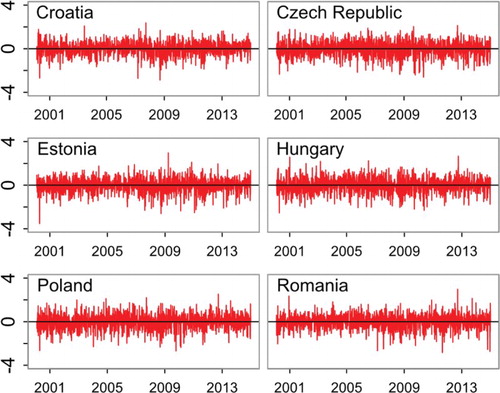
All of the co-exceedances are on average negative and are negatively skewed in most of the cases (except Hungary); thus, joint extreme negative shocks are more common in our examined time period. Interestingly, the lowest joint negative returns occurred in all of the markets at almost the same time: 10 October 2008 (for the Czech Republic, Estonia, Poland and Romania), 16 October 2008 (Hungary) and 20 November 2008 (Croatia). All of these days correspond to the peak of the recent financial crisis. Joint positive shocks were also recorded in autumn 2008 (although for Estonia only in March 2009), thus demonstrating the extremely high volatility of returns during this period.

The co-exceedances display very low autocorrelation, which is practically zero in all of the cases. Therefore, this measure of stock market co-movement is not persistent, in contrast to, for example, the dynamic conditional correlations from multivariate GARCH models. Using co-exceedances might therefore be beneficial from a methodological perspective as well because highly correlated time series in regressions usually lead to large size distortions, and even if robust standard errors are applied, the model remains mis-specified (see Granger, Hyung, and Jeon 2001; Su 2008).

The return co-exceedances in Figure 1 do not appear to have any clear, specific pattern because before calculating the co-exceedances, when the returns are filtered via the ARMAX-EGARCHX models. It is therefore of particular interest whether we are able to measure any systematic effects on the return co-movement even after such a strong filtration procedure. A reader may compare Figure 1 with Figure A1 in the Appendix, where the return co-exceedances are calculated for non-filtered returns. There are sizeable differences, as we can observe large variability in the return co-exceedances during the recent crisis period in Figure A1 in Appendix, but not in Figure 1. As a consequence, we conduct a robustness check to examine whether the regression results (presented in the following sub-section) are influenced by the different filtering procedure.

Figure 1. Return co-exceedances from standardized residuals.

5.2. Evidence of financial contagion: full sample

In Table 2, we provide the results from the quantile regressions based on the co-exceedances computed from the standardized residuals through the ARMAX-EGARCH model. Because we focus on contagion, we present the results from the left-tail of the return co-exceedances.¹² All of the asymmetric terms of the expected and unexpected volatilities are highly significant (γ₂, γ₄). In addition, all of the coefficients are negative, suggesting that an increase in both expected and unexpected volatility accompanied with market declines tends to produce negative joint co-movements. The size of this effect is larger in the left-tails and it gradually weakens through the other quantiles, although it remains significant, even in the OLS estimates.

Table 2. Quantile regression estimates: co-exceedances based on standardized residuals.

	τ	β0	β1	γ1	γ2	γ3	γ4	δ1	δ2	λ1	λ2	ν1	ν2	η1	η2	ϕ1	ϕ2	υ1	R^2
	0.01	−7.88	−0.25	−0.30	−169.42^d	−0.70	−163.92^d	170.38	122.37	1.39	31.83	122.91	−119.64	−11.17	9.19	79.39	28.73	1.11	0.48
	0.05	−0.12	0.04	0.04	−110.15^d	0.00	−95.89^d	0.40	−0.27	0.02	−0.83	0.78	−0.53	0.10	0.09	1.55	−1.00	−0.02	0.42
	0.10	−0.10^d	0.01	0.04^a	−77.64^d	0.02	−73.68^d	0.51	−3.24	0.02^b	−0.61	0.30	−0.77	0.20	0.25	0.53	0.05	−0.01	0.39
	0.25	−0.01	0.01	0.03	−39.78^d	0.00	−42.89^d	0.21	−6.08	0.01	−1.01	−0.42	−1.25	0.10	0.59	0.96^a	0.01	0.00	0.20
	OLS	6.21^d	−4.33^a	16.01^d	−38.69^d	11.82^d	−32.23^d	68.61	−460.61	2.98^d	−76.86	−6.49	−146.58^b	−2.26	31.10	123.73^b	−1.17	0.06	0.28
Croatia
	0.01	−8.70	−1.16	−1.87	−205.12^d	−1.47	−214.66^d	276.10	169.10	1.92	323.35	−12.33	−441.30	−21.96	8.37	10.22	63.05	0.18	0.42
	0.05	−0.28	−0.02	0.08	−133.63^d	0.04	−140.18^d	−1.18	9.33	0.09	3.37	−0.60	−7.55	−2.49	−0.71	0.22	−1.08	0.00	0.37
	0.10	−0.11	−0.03	0.03	−95.62^d	0.03	−98.30^d	0.30	0.97	0.02	0.34	0.28	−0.27	−0.28	−0.05	0.58	−0.11	0.01	0.35
	0.25	−0.06^b	−0.03	0.02	−48.40^d	0.03	−52.74^d	0.43	6.55	0.01	3.47	−1.06	−0.35	−0.62	−0.34	0.49	−1.06	0.00	0.24
	OLS	2.28	−5.93^c	18.50^d	−48.67^d	17.90^d	−44.50^d	−14.15	413.57	3.38^c	119.52	14.31	−91.47	−33.80	7.95	127.59^a	−42.46	−0.60	0.30
Czech Republic
	0.01	−9.54	−0.29	−1.18	−178.33^d	−0.13	−171.98^d	45.76	−70.94	0.98	237.12	−76.00	−492.97	−3.15	41.38	70.76	101.51	3.25	0.43
	0.05	−0.12	0.00	0.00	−122.56^d	−0.02	−102.57^d	2.28	9.05	0.04	2.22	−0.86	−10.46	0.16	−0.01	0.91	0.92	−0.01	0.41
	0.10	−0.10^d	−0.01	0.04	−89.38^d	0.03	−85.75^d	1.28	−2.35	0.02^a	−0.42	−0.39	−1.07	0.16	0.24	0.60	0.03	−0.01	0.38
	0.25	−0.05	−0.01	0.04	−48.34^d	0.04^a	−43.83^d	−0.60	3.48	0.01	−0.68	−0.83	0.54	0.05	0.34	1.03	−0.28	−0.02	0.24
	OLS	2.83	−6.75^d	16.69^d	−44.55^d	12.03^d	−37.21^d	81.15	266.37	4.27^d	−58.68	−4.03	−84.07	2.93	38.12	150.73^b	5.09	−0.84	0.31
Estonia
	0.01	−24.95^b	2.35	11.49	−166.54^d	3.35	−152.28^d	118.82	−47.37	0.25	−99.07	−80.23	−318.32	86.02	−30.93	67.93	143.80	−2.25	0.38
	0.05	−0.41	0.12	0.22	−125.67^d	0.01	−124.23^d	−5.30	3.96	0.04	0.86	−1.16	−9.41	−1.16	−1.74	−1.36	0.95	0.05	0.38
	0.10	−0.10^d	0.02	0.01	−91.82^d	0.02	−82.93^d	−1.06	−0.76	0.00	0.47	−0.65	−0.50	−0.31	0.34	0.40	0.28	0.01	0.36
	0.25	−0.03	0.03	0.01	−46.60^d	0.01	−42.66^d	−0.70	0.79	−0.01	0.64	−0.50	−2.35^c	0.06	0.41	0.67	0.57	−0.01	0.23
	OLS	2.77^a	−0.97	18.32^d	−47.17^d	18.98^d	−42.91^d	−19.00	−38.81	2.76^b	35.13	−31.11	−38.06	−53.66	36.61	84.27	29.14	−1.64	0.29
Hungary
	0.01	−25.39^b	3.31	5.03	−179.25^d	1.47	−163.29^d	11.02	12.40	0.99	162.50	−188.75	−489.78	15.04	44.18	86.51	100.07	−10.21^a	0.39
	0.05	−0.18	0.02	0.04	−132.62^d	0.00	−109.87^d	−0.95	2.35	0.05	1.80	−2.67	−5.13	−1.18	−0.17	−0.78	−0.03	−0.02	0.38
	0.10	−0.10^d	0.00	0.03	−95.17^d	0.01	−82.23^d	0.41	0.31	0.02	0.80	−0.48	−1.01	−0.27	0.00	−0.09	−0.01	0.00	0.37
	0.25	−0.05^c	0.01	0.01	−47.50^d	0.03	−56.09^d	−0.27	2.26	0.01	1.60	−0.15	−1.09	−0.12	0.31	0.33	−0.24	0.00	0.22
	OLS	3.08^a	−2.53	18.68^d	−46.09^d	15.29^d	−42.25^d	−92.83	301.62^a	2.71^b	98.08	−20.34	−116.89	−67.13^a	−27.26	105.55	−17.81	−0.89	0.28
Poland
	0.01	−9.61	1.63	2.07	−183.96^d	1.65	−191.72^d	39.83	−20.63	0.85	91.97	27.39	−124.55	19.92	9.92	114.10	−75.77	3.37	0.41
	0.05	−0.25	−0.11	0.00	−123.76^d	0.01	−111.76^d	1.75	−3.10	0.06	1.93	−1.32	−4.65	1.14	0.56	4.77	−0.83	0.08	0.39
	0.10	−0.11	−0.02	0.01	−89.22^d	0.02	−81.36^d	−0.07	−1.10	0.02	0.16	−0.17	0.29	0.18	0.26	1.62	−0.71	0.01	0.36
	0.25	−0.05^c	0.00	0.00	−43.07^d	0.01	−39.43^d	0.44	0.38	0.02^b	0.26	0.35	−0.22	−0.24	0.50	1.14^b	0.02	0.01	0.21
	OLS	3.25^a	−5.43^c	15.87^d	−39.65^d	11.23^d	−33.25^d	100.63	82.92	4.81^d	13.99	4.82	−215.72^c	−31.50	24.24	211.27^c	25.11	1.39	0.28
Romania

Notes: τ denotes respective quantile. The coefficient constants β₁, δ₁, ν₁, η₁, ϕ₁, υ₁ are multiplied by100. Significance at 10%, 5%, 1% and 0.1% is denoted by ‘a’, ‘b’, ‘c’ and ‘d’ superscripts, respectively. For the quantile regressions, R² denotes the pseudo R² as defined in Koenker and Machado (1999, Equation (7)), while for the OLS regressions, the usual adjusted coefficient of determination is used. The standard errors of the estimated OLS regression coefficients were derived from the HAC matrix and calculated using the quadratic spectral kernel weighting scheme with automatic bandwidth procedure, as in Newey and West (1994).

Within our definition of contagion, the sum of the estimated coefficients of unexpected volatility and its asymmetric term should be negative (γ₃ + γ₄). According to our findings, this result holds in all cases; thus, unexpected events coupled with market declines increase the size of extreme market co-movements. As a consequence, our results suggest that contagion from the US market to the CEE region has taken place.

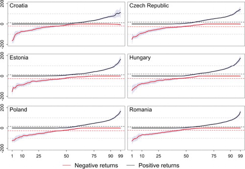
Figure 2 shows the striking difference in the size of the coefficients of unexpected volatility with respect to the different predicted quantiles, including those in the right-tail of the co-exceedance distribution. We can clearly see that the unexpected part of the market’s volatility matters not only for contagion (negative return co-exceedances) but also for positive return co-exceedances. Baur and Fry (2009) distinguish between positive and negative contagion and Baur (2013, p. 793) argues, that

… a crisis-specific increase in the degree of dependence in the right-tail of the distribution is less problematic than a crisis-specific increase in the degree of dependence in the left-tail of the distribution. Contagion is usually associated with falling stock prices and negative returns and thus is better characterized by an increased lower quantile or left-tail dependence than an upper quantile or right-tail dependence.

Therefore, we focus on the left-tail dependence only, but the detailed results for right-tail co-exceedances are available in Online Appendix. These results show that an unexpected increase in market volatility during bullish market conditions spills over to the CEE markets in a similar fashion as the negative returns. Therefore, our results are broadly in line with Dungey and Gajurel (2015), who – examining sample of 54 countries using the factor type model of contagion – find that contagion is a common phenomenon.

Figure 2. Unexpected market volatility effects at different quantiles.

Notes: The figure reports the size of coefficients from quantile regression results for quantiles (τ) from 1 to 99. Negative returns correspond to the sum of two coefficients (γ₃ + γ₄), while positive returns are just γ₃. The horizontal dashed lines represent OLS coefficient estimates.

Regarding the fundamental variables that we control for in our regressions, only a few of them are significant. This result justifies our view that most extreme market co-movements are investor over-reactions rather than fundamentally based decisions.

Several fundamentals are significant for the OLS estimates, but these results should not be overemphasized because they capture the average conditions in the stock markets rather than the extremes, which is our focus. The STOXX 1800 index returns are statistically significant in all countries and the coefficient λ₁ is positive, which is in line with our expectations that if world-wide stock prices increase, it is likely that national stock markets will increase as well. The other fundamentals are significant only for certain countries, including the volatility of gold (significant in Croatia and Romania) and bond yields (significant in Croatia, the Czech Republic, Estonia and Romania).

5.3. Is contagion a financial crisis phenomenon?

Bekaert et al. (2014) find that financial contagion from the US stock market to the CEE markets occurred during the financial crisis. These results are intuitive and are supported by most of the literature finding excess co-movement during the crisis period. Therefore, we examine: (1) whether our results are driven only by the recent financial crisis and (2) whether, in case that we observe contagion in both good and crisis times, contagion is stronger during the crisis.

5.3.1. Contagion in good times

We re-estimate the quantile regression models for two periods. The first period ends in June 2007, and the second period starts after March 2009 (crisis period is excluded). This division is similar to that presented in Baur (2012), Kontonikas, MacDonald, and Saggu (2013) and Florackis, Kontonikas, and Kostakis (2014). However, it is noteworthy that the comparison of these results with the results for full sample is not straightforward, as the corresponding quantiles will change. Despite that, it represents an important check whether financial contagion occurs only in specific periods such as financial crisis or whether it is a more general phenomenon occurring in good times too.

Our main results remain largely unchanged, as before and after the crisis period all of the coefficients of the asymmetric unexpected market volatility of the models predicting the left-tail of the return co-exceedances remain negative and statistically significant.¹³ In addition, after the 2007–2009 crisis, the sensitivity of the CEE stock markets has increased, that is, when the markets plummet, a unit change in unexpected market volatility now leads to higher extreme market co-movements.

5.3.2. Contagion during financial crisis

We examine whether extreme negative co-exceedances are more intensively related to the unexpected market volatility during the recent financial crisis. We extend the specification in Equation (10) by the regime dependent expected and unexpected market volatilities in the following way. We introduce two additional dummy variables to characterize the crisis regime and after-crisis regime. D₁ is equal to 1 for observations in the crisis (July 2007–March 2009), 0 otherwise. D₂ is equal to 1 if the observation is from the after-crisis period, that is, from April 2009 onward, 0 otherwise. As a result, our regression specification is as follows: (11) where (12) We report the results in Table 3. For the sake of simplicity, we do not present the estimates of β (available in the Online Appendix) and focus instead on the estimates of expected and unexpected market volatilities, that is, Γ, D₁Γ and D₂Γ. These coefficients are denoted in Table 3 as γ₁, γ₂, γ₃, γ₄ for the first regime characterized by D₁ (γ₁ – expected market volatility, γ₂ – expected market volatility with decreasing markets, γ₃ – unexpected market volatility and γ₄ – unexpected market volatility with decreasing markets), γ₅, γ₆, γ₇, γ₈ denote the change in coefficients during the crisis period, and γ₉, γ₁₀, γ₁₁, γ₁₂ denote the change in coefficients (compared to the pre-crisis period) after the crisis. The coefficient γ₈ denotes the change in the effect of the unexpected market volatility when markets are decreasing, which is of prime interest for this study.

Table 3. Quantile regression re-estimates according to crisis period: co-exceedances based on standardized residuals.

		Before the financial crisis				During the financial crisis				After the financial crisis
	τ	γ1	γ2	γ3	γ4	γ5	γ6	γ7	γ8	γ9	γ10	γ11	γ12	R^2
Croatia	0.01	−0.34	−148.52^d	−0.40	−91.53^d	0.38	−49.76^b	0.81	−128.89^c	−0.39	25.20^a	−0.67	15.37	0.72
	0.05	0.01	−97.80^d	0.01	−98.30^d	0.00	−45.64^c	−0.01	−61.44	0.00	14.83^b	0.00	40.53^b	0.57
	0.10	0.04	−74.10^d	0.01	−81.61^d	0.01	−42.56^c	0.03	−24.52	−0.01	9.80	0.01	34.65^b	0.47
	0.25	0.03	−33.19^d	0.02	−38.10^d	0.02	−27.43^d	0.01	−31.09	0.01	−6.10	0.03	−0.51	0.25
	OLS	24.14^d	−42.09^d	13.73^c	−35.23^d	2.89	−10.12	11.42	−20.42	−0.45	2.93	−6.06	15.87	0.35
Czech Republic	0.01	0.03	−152.27^d	−0.02	−123.88^d	0.01	−46.59^a	0.07	−101.67^a	0.00	−4.30	0.03	−2.68	0.68
	0.05	0.06	−111.09^d	0.03	−96.63^d	−0.01	−17.16	−0.01	−28.77	−0.01	−13.57	−0.02	−29.92	0.55
	0.10	0.01	−85.18^d	0.02	−81.05^d	0.00	−24.20^a	0.05	−44.46	−0.01	−11.48	−0.02	−8.66	0.46
	0.25	0.05	−46.21^d	0.04	−36.01^d	0.00	−14.80^b	0.10	−39.60^a	−0.04	0.77	−0.02	−11.91	0.28
	OLS	28.64^d	−54.49^d	23.65^d	−46.15^d	2.29	−10.58^a	3.21	−7.48	−2.59	0.76	−11.68	0.49	0.40
Estonia	0.01	−0.07	−158.21^d	−0.11	−109.94^d	0.01	−45.59^a	0.11	−121.57^a	−0.23	−24.72	−0.22	−69.23^a	0.71
	0.05	0.01	−112.45^d	−0.02	−89.54^c	0.02	−14.89	0.01	−1.91	0.01	−14.58	0.03	−34.33	0.57
	0.10	0.07	−79.89^d	0.03	−66.05^d	−0.01	−29.62^d	−0.05	−21.03	0.00	−21.00^b	0.01	−32.64	0.50
	0.25	0.09	−42.56^d	0.06	−32.48^d	−0.01	−26.34^d	−0.06	−45.12^c	−0.01	−8.77^a	0.02	−15.57	0.30
	OLS	26.51^d	−47.73^d	7.01^a	−31.31^d	−4.62	−9.63^a	13.76^a	−25.63^b	2.96	−8.23	19.51^a	−28.06	0.43
Hungary	0.01	0.15	−150.41^d	0.05	−104.43^d	0.12	−22.69	0.00	−76.27^a	−0.05	−8.20	−0.10	−18.09	0.67
	0.05	0.04	−113.09^d	0.02	−68.72^d	−0.01	−14.94	−0.03	−75.67	0.00	−1.87	−0.03	−47.44^b	0.54
	0.10	0.02	−88.74^d	0.02	−74.21^d	0.00	−19.39	−0.03	−8.28	−0.01	4.64	−0.02	−10.25	0.45
	0.25	0.05	−46.40^d	0.02	−39.01^d	−0.02	−5.56	0.00	3.11	−0.03	5.49	0.03	−8.64	0.24
	OLS	25.90^d	−56.88^d	23.85^d	−47.27^d	−0.71	−5.41	−0.52	5.89	−4.92	9.17^a	−7.07	−3.11	0.35
Poland	0.01	0.13	−161.87^d	−0.01	−108.40^d	−0.05	−5.74	0.10	−36.99	−0.30	−18.68	−0.15	−10.78	0.66
	0.05	0.02	−121.28^d	0.00	−88.01^d	0.00	−5.09	0.00	−33.31	0.00	14.65^a	−0.01	−15.41	0.54
0.10	0.00	−95.47^d	0.00	−70.21^d	0.02	−4.83	0.00	−51.09^b	0.02	14.83^b	0.00	−4.51	0.46
	0.25	0.01	−51.44^d	0.02	−52.91^d	−0.01	−5.47	−0.03	−38.56^b	0.00	12.55^b	−0.01	13.26	0.25
	OLS	27.59^d	−57.52^d	22.49^d	−50.05^d	−0.48	2.07	−7.10	−7.61	−1.64	10.16^b	−4.53	9.70	0.36
Romania	0.01	0.04	−146.15^d	0.03	−100.46^d	0.04	−42.41^b	0.02	−137.84^b	0.00	−20.01	−0.02	−19.09	0.70
	0.05	0.02	−97.44^d	0.00	−88.72^c	−0.01	−35.16^b	0.00	−17.86	−0.01	−27.31^b	0.00	−12.69	0.54
	0.10	0.04	−70.74^d	0.01	−43.29^c	0.00	−46.42^d	0.02	−65.45^b	0.00	−18.68^b	0.02	−32.97^a	0.46
	0.25	0.04	−30.21^d	0.03	−20.35^b	0.00	−34.82^d	0.01	−49.40^c	0.02	−14.72^d	0.03	−34.86^c	0.25
	OLS	16.41^d	−35.93^d	6.43^b	−15.92^c	2.83	−17.94^b	14.22	−48.02^c	10.96^b	−17.59^d	6.34	−27.30^b	0.38

Notes: As for Table 2.

The results in Table 3 support findings reported in the literature that co-exceedances are higher during the crisis period as follows: (i) almost all γ₈ coefficients are negative, suggesting that the sensitivity to unexpected negative events increased, that is, extreme negative co-exceedance is higher for the same magnitude of ‘bad surprise’ shock during the financial crisis, (ii) compared to the γ₄ coefficient, the absolute value of the γ₈ coefficient for the most extreme quantile (0.01) is large (note that the overall effect is the sum γ₄ + γ₈, so that γ₈ denotes only the change), (iii) the γ₈ coefficient for the extreme lower quantile is statistically significant at least at 10% for all countries except for Poland.

5.4. Robustness analysis

5.4.1. Has return filtration induced spurious contagion?

Filtering returns via the ARMAX-EGARCHX model might be considered too fine an approach to obtain residuals, and critics may argue that it distorts the ‘true’ relationship between markets. We re-estimate our quantile regression models but with return co-exceedances calculated from standardized raw returns (E[r_t] = 0, V[r_t] = 1). The results for these non-filtered return co-exceedances are available in Table A1 in the Appendix.

Our main results again remain largely unchanged. An interesting observation is that the effects are slightly lower, as the negative coefficients of unexpected market volatilities are higher. It appears that although fluctuations in other markets seem to mitigate contagious tendencies from the US stock market toward the CEE stock markets, they are not sufficient to eliminate the contagion.

5.4.2. Are results sensitive to model specifications?

Next, we investigate sensitivity of our results to the different regression model specifications. In the first specification, we include only the constant, the lagged return co-exceedance and the expected and unexpected market volatilities. Therefore, we exclude fluctuations in other markets and the policy index (see Equation (13)). The results remain largely unchanged: (13) Previous findings led us to the second alternative specification, where we have included the constant and the lagged return co-exceedance together with variables capturing movements on other markets including the news-based economic policy uncertainty index, thus excluding expected and unexpected US market volatilities: (14) Contrary to the full model specification (Equation (10)), several variables become statistically significant across the whole range of quantiles for almost all countries especially global STOXX returns and its expected volatility, government bonds and the expected volatility in the oil market. We find foreign exchange market important for the extreme negative co-exceedances for Croatia, Estonia and Romania, and gold market for the Czech Republic, Hungary, Poland and Romania.

We compare the pseudo R² (Koenker and Machado 1999) between Equations (10) and (14) to assess whether the inclusion of the expected and unexpected market volatility improves the fit of regressions. With the exception of the very extreme quantiles of 0.01, where the fit is comparable, the fit of the full model (Equation (10)) is superior because the average pseudo R² is approximately 2.5 times higher for all left-tail quantiles (0.01, 0.05, 0.10, 0.25) and for all countries. These results indicate that expected and unexpected market volatility helps understand the joint occurrence of extreme events in stock markets.

6. Concluding remarks

We analyze financial contagion in emerging markets using a new approach for measuring contagion, which stipulates that contagion should be observed as excess co-movement during negative unexpected events. More specifically, we examine whether unexpected negative events in the US stock market propagate into emerging stock markets and increase the co-exceedance between these markets and the US market. We interpret the results as evidence of financial contagion. Using quantile regressions, we specifically examine those periods when the US market experienced the largest declines. We use the co-exceedance measure introduced by Bae, Karolyi, and Stulz (2003) and a quantile regression framework, as in Baur and Schulze (2005), but we extend these two contributions by decomposing US stock market volatility into expected and unexpected components and examining how this unexpected volatility component increases the co-exceedance between stock markets.

Using our approach with daily data from 1998 to 2014, we find evidence of financial contagion for all of our examined emerging markets (Croatia, the Czech Republic, Estonia, Hungary, Poland and Romania). Therefore, the contagion is present regardless of the monetary policy regime the countries adopted. We subject this finding to a series of robustness checks.

First, we investigate whether our results hold for different time periods, that is, before and after the 2007–2009 crisis and we confirm that contagion occurs both during the financial crisis and in good times. However, we find that contagion is stronger during the crisis. Second, instead of filtering the stock market returns through the ARMAX-EGARCHX model, we use non-filtered returns, but the results remain unchanged. Third, we control for the returns and volatilities of different asset classes – gold, oil, foreign exchange and government bonds. We observe that extreme negative co-movements are not driven by fluctuations in these markets, thus providing further evidence that the contagion is based on investor over-reactions rather than on fundamentally based decisions.

Overall, our results indicate that financial contagion from the US stock market to the CEE markets occurs irrespective of the financial crisis period but we find that contagion is stronger during the crisis (sensitivity to unexpected negative events increases considerably), that is, a result, which goes in the direction of findings by Asongu (2012) or Bekaert et al. (2014). As noted by Dungey and Gajurel (2015), reducing the potential for idiosyncratic contagion can importantly reduce the consequences for the domestic economy. However, tempting to reduce contagion using certain micro or macroprudential policy measures crucially depends on the effectiveness of these measures.

In terms of future research, it would be worthwhile to develop more structural approaches to assess financial contagion so that they can be systematically used for policy analysis at various institutions, such as international organizations, governments or central banks.

Acknowledgement

We thank Jozef Baruník, Jarko Fidrmuc, Ľuboš Pástor, participants at the Slovak Economic Association Meeting 2015, The Joint Conference on Institutional Investors/Hedge Funds and Emerging Market Finance (Ghent University, Belgium), The 14th INFINITI Conference on International Finance (Trinity College Dublin, Ireland) and Czech National Bank-Institute of Economic Studies conference on Challenges for Financial Stability in Europe for useful comments.

Disclosure Statement

No potential conflict of interest was reported by the authors.

Additional information

Funding

We appreciate the support provided by the Slovak Grant Agency for Science (Vedecká grantová agentúra, VEGA) [grant number 1/0392/15]. This work was supported by the Slovak Research and Development Agency (Agentúra na podporu výskumu a vývoja) [contract no. APVV-14-0357].

Notes

†The Online Appendix is available at http://ies.fsv.cuni.cz/en/staff/horvath.

1 See, for example, the financial stability reports of the respective countries’ central banks (Czech National Bank 2015; National Bank of Poland 2015), which show that local banks are well capitalized and are able to withstand large negative shocks.

2 More specifically, Bae, Karolyi, and Stulz (2003) define financial contagion as the fraction of extreme returns that are not explained by fundamentals but rather by extreme returns in another country/region. Extreme returns are those below the 5th or above the 95th quantile of the marginal return distribution and are referred to as return exceedances. Co-exceedances are defined as the joint occurrence of i exceedances of positive or negative returns on a given day.

3 This approach is also used by Koch (2014), who first filters the return series using a VAR model with exogenous, potentially common factors (e.g. S&P 500 equity index, credit spread) and only then studies extreme return co-exceedances in energy markets (WTI crude oil, heating oil, gasoline, natural gas, etc.).

4 Common shocks driving co-movement are described as ‘monsoonal effects’ by Masson (1999).

5 We estimate several ARMAX(p, q)-EGARCHX(r, f) models with orders p, q, r, f up to 2. We select those models for which the resulting standardized residuals do not display autocorrelation and conditional heteroscedasticity. For this purpose, we use the test developed by Peña and Rodríguez (2006) using Monte Carlo critical values (see Lin and McLeod 2006). If more suitable models remain, we prefer the more parsimonious models, that is, those with the least number of estimated parameters (p + q + r + f). If necessary, the chosen specification is selected using the Bayesian information criterion (BIC, Schwartz 1978). Because we are unable to identify fully suitable models for Estonian and Romanian stock market returns, we choose the final specifications according to the BIC criterion. For both Estonia and Romania, the autocorrelation of first order of standardized residuals was statistically significant, but the dependence is small 0.052 for Estonia and just 0.049 for Romania. For Romania statistically significant ARCH effects are identified as well, but only with a test testing up to 20 lags. Therefore, we consider our filtering procedure to be reasonable also for these two markets.

6 Within the κ₂ test, the estimation of the variance of squared demeaned returns is conducted via the non-parametric long-run variance estimator with automatic bandwidth selection of Newey and West (1994) and the Bartlett kernel weighting scheme. The same approach is used by Dungey and Gajurel (2014) to identify crisis and non-crisis periods in equity markets, and Dungey and Gajurel (2015) to define banking crisis periods. The script, including the ICSS algorithm of Inclán and Tiao (1994), is coded in R and is available upon request.

7 As a robustness check, we re-run the filtering equations using the normality distribution as well. The resulting standardized residuals were highly correlated with those used in the study for calculation of return co-exceedances (correlation coefficients were within the 0.9934–0.9995 range). We therefore conclude that our results are robust with respect to the choice of the distribution.

8 With daily data, range-based variance estimators have a much higher efficiency compared with the simplest estimator of the daily variance , that is, the Garman and Klass (1980) estimator is 7.4 times more efficient. For a more detailed treatment of range-based estimators, see Molnár (2012) or McLeish (2002).

9 To check the robustness of our forecasts, we forecasted variance also with estimation windows of sizes 252 and 1000. The forecast based on previous 252 trading days correlates with the forecasts based on previous 500 trading days significantly as the correlation coefficient is 0.984. The forecast based on previous 1000 trading days also correlates with the forecasts based on previous 500 trading days significantly as the correlation coefficient is 0.995. We therefore conclude that in our setting, the expected market variance is robust to the choice of the estimation window.

10 For a few instances where the predicted volatility is negative, the value of the expected volatility is set to 0. This approach is also visible from descriptive statistics in Table 1, where there are 31 instances where forecasted market volatility is set to 0, that is, the minimum value.

11 These results are available as part of the Online Appendix. For some markets, the value of return co-exceedances is zero in nearly 50% of all observations. For this reason, we add jitter to the return co-exceedances by replacing 0-valued return co-exceedances with a random value from −0.001 to +0.001. Because the return co-exceedances are calculated from standardized residuals with mean 0 and variance of approximately 1, these imputed values are small and distort the overall distribution of co-exceedances only negligibly but improve the convergence of our estimator.

12 The results for the right-tail of the return co-exceedance distribution are available in the Online Appendix.

13 The complete results from Sections 5.3 and 5.4 are available in the Online Appendix.

Appendix

Figure A1. Return co-exceedances from non-filtered returns.

Note: Returns are not filtered but are standardized to E[r_t] = 0 and V[r_t] = 1.

Table A1. Quantile regression estimates: co-exceedances based on non-filtered returns.

	τ	const.	β1	γ1	γ2	γ3	γ4	δ1	δ2	λ1	λ2	ν1	ν2	η1	η2	ϕ1	ϕ2	υ1	R^2
0.01	−0.53	−0.31	0.46	−151.11^d	−0.25	−134.03^d	35.16	83.88	0.38	−75.75	−14.17	−46.36	2.66	−5.97	6.76	14.11	−0.09	0.68
0.05	−0.02	0.07	0.32	−102.90^d	0.06	−90.46^d	2.97	6.60	0.03	−35.60	0.53	−5.50	0.29	−0.45	0.56	1.99	−0.01	0.54
0.10	−0.04	0.02	0.06	−79.31^d	0.01	−72.14^d	0.38	4.46	0.01	−4.75	0.14	−1.84	0.14	−0.40	0.35	0.33	0.00	0.45
0.25	0.01	0.03	0.02	−39.69^d	0.02	−45.36^d	0.12	−1.36	0.01	−2.05	−0.63	−1.25	0.35	0.42	1.18^a	0.03	0.01	0.24
OLS	3.96^a	−3.00	25.96^d	−45.00^d	16.56^d	−37.72^d	56.14	−441.79	3.27^c	−471.17^b	−156.22	−260.67^b	2.67	30.74	155.67^b	69.38	0.59	0.34
Croatia
	0.01	−0.08	−0.01	−0.01	−167.54^d	−0.01	−150.33^d	1.94	1.81	0.02	0.78	−0.62	−2.27	0.61	−0.41	0.07	0.19	0.01	0.67
	0.05	−0.07	−0.04	0.10	−120.84^d	0.04	−120.90^d	−1.16	5.48	0.02	−7.63	−0.36	−3.32	0.16	−0.02	0.54	−0.53	−0.01	0.55
	0.10	−0.05	−0.02	0.05	−95.10^d	0.04	−90.63^d	0.22	5.38	0.02	−5.72	−0.39	−0.98	0.69	0.27	1.07	−0.72	0.00	0.46
	0.25	0.02	−0.03	0.02	−49.81^d	0.03	−51.29^d	0.01	3.47	0.01	−3.11	−1.43	−0.60	0.32	0.46	1.47	−0.11	0.00	0.27
	OLS	1.01	−6.97^b	29.59^d	−58.12^d	21.91^d	−48.22^d	−115.76	857.66^b	3.53^c	−259.81	−88.22	−128.19	12.36	−10.10	238.29^c	−74.30	−0.40	0.40
Czech Republic
	0.01	−0.08	−0.07	−0.05	−172.49^d	−0.06	−154.42^d	−1.99	12.00	0.05	−1.37	−0.09	−4.22	0.24	−0.08	3.95	−3.87	−0.02	0.70
	0.05	−0.07	−0.01	0.02	−120.77^d	0.00	−97.68^d	−0.81	2.89	0.03	−3.20	0.14	−0.86	0.27	0.10	2.18	−0.78	0.00	0.57
	0.10	−0.04	0.01	0.08	−94.48^d	0.03	−87.04^d	0.24	10.17	0.03	−9.39	−0.40	−1.86	0.15	0.14	2.24	−0.48	0.01	0.48
	0.25	0.01	−0.06	0.10	−51.71^d	0.05	−49.61^d	0.46	4.53	0.07	−11.64	−0.79	−1.49	0.76	1.14	2.83	0.36	0.00	0.29
	OLS	2.62	−8.38^b	25.44^d	−52.70^d	16.67^d	−46.24^d	243.92	758.52	7.93^d	−571.44^d	−49.97	−218.44	49.56	44.57	266.12^c	50.34	−0.86	0.42
Estonia
	0.01	−0.70	0.48	1.97	−155.90^d	0.05	−141.61^d	14.82	16.39	0.04	−83.56	25.19	−216.91	1.66	−9.69	1.93	38.22	−0.24	0.66
	0.05	−0.08^d	0.01	0.04	−116.85^d	0.01	−107.20^d	−0.59	−0.97	0.01	−2.24	−0.30	−0.87	0.01	−0.17	0.26	0.26	0.00	0.53
	0.10	−0.06^d	−0.01	0.03	−90.94^d	0.01	−73.65^d	0.30	0.30	0.02^b	−2.99	−0.46	−0.23	0.13	−0.05	0.11	0.20	0.00	0.45
	0.25	0.00	−0.01	0.04	−45.15^d	0.03	−43.03^d	−0.97	1.97	0.00	−1.78	−0.32	−0.98	0.04	−0.14	0.22	−0.33	0.00	0.24
	OLS	0.91	−0.06	24.11^d	−56.72^d	21.80^d	−46.51^d	−493.39^b	−194.43	0.22	172.53	−120.24	−145.90	−50.62	54.56	94.10	74.87	−0.87	0.35
Hungary
	0.01	−0.37	0.05	0.02	−170.69^d	−0.05	−125.01^d	−8.95	−22.74	0.06	4.67	0.56	−1.47	−1.02	0.62	−3.15	3.12	−0.05	0.65
	0.05	−0.10^d	−0.02	0.03	−116.36^d	0.00	−100.21^d	−0.62	1.52	0.02^a	−2.81	−0.89	0.12	0.04	0.04	0.09	−0.11	−0.01	0.53
	0.10	−0.06^d	−0.01	0.02	−92.85^d	0.01	−82.99^d	−0.79	2.56^a	0.01	−2.04	−0.51	−0.63	−0.19	0.14	0.06	−0.40	−0.01	0.46
	0.25	−0.01	0.00	0.02	−48.27^d	0.01	−54.42^d	−1.94^a	0.61	0.00	−0.01	−0.35	−0.71	−0.29	−0.20	−0.28	0.17	−0.01	0.24
	OLS	0.23	−2.97	28.40^d	−54.18^d	19.33^d	−50.18^d	−322.20^b	218.29	1.02	13.38	52.54	−166.16	−89.00^b	−32.95	155.02^b	11.78	−0.06	0.36
Poland
	0.01	−0.12	−0.04	0.03	−162.05^d	0.03	−127.26^d	−0.75	0.71	0.03	1.74	−4.17	−18.40	0.65	0.02	1.73	2.74	0.05	0.68
	0.05	−0.07^a	0.00	0.05	−119.30^d	0.01	−100.38^d	−0.91	−1.03	0.02	−4.19	−0.34	−1.89	0.22	0.08	0.73	0.25	0.01	0.53
	0.10	−0.07^c	0.01	0.04	−83.82^d	0.02	−66.62^d	0.31	−0.26	0.02^a	−3.01	−0.07	−0.46	−0.16	0.23	0.97	0.10	0.02^a	0.44
	0.25	0.00	0.01	0.03	−41.73^d	0.04^a	−49.53^d	0.22	−0.24	0.01	−1.43	0.00	−1.68	−0.15	0.24	1.63^b	0.27	0.01	0.23
	OLS	2.89	−2.77	20.89^d	−45.62^d	12.66^c	−37.47^d	125.81	−99.59	5.03^d	−104.01	−29.45	−310.13^c	−37.77	42.10	311.60^d	73.15	1.78^b	0.36
Romania

Notes: τ denotes respective quantile. The coefficients const, β₁, δ₁, ν₁, η₁, ϕ₁, υ₁ are multiplied by100. Significance at 10%, 5%, 1% and 0.1% is denoted by ‘a’, ‘b’, ‘c’ and ‘d’ superscripts, respectively. For the quantile regressions, R² denotes the pseudo R² as defined in Koenker and Machado (1999, Eq. 7), while for the OLS regressions, the usual adjusted coefficient of determination is used. The standard errors of the estimated OLS regression coefficients were derived from the HAC matrix and calculated using the quadratic spectral kernel weighting scheme with automatic bandwidth procedure, as in Newey and West (1994).

Table A2. Estimation of filtered returns: ARMAX-EGARCHX model estimates.

	Croatia	Czech Republic	Estonia	Hungary	Poland	Romania	US
Mean equation
µ (×100)	0.019	0.024	0.016	0.015	0.007	0.061	−0.010
φ1	0.916^d	0.923^d	1.840^d			0.225^d
φ2			−0.847^d			−0.983^d
θ1	−0.898^d	−0.903^d	−1.739^d	0.005	0.005	−0.106^d	−0.054^d
θ2		−0.006^a	0.673^d			0.962^d
θ3			0.078^d			0.124^d
Additional mean equation variables
Returns on the FOREX,	0.043	−0.058^b	0.060^d	−0.095^d	−0.074^b	0.046^a	0.735
Returns on the STOXX,	0.046^d	0.011	0.068^d	−0.025	−0.047	0.041^d	6.761^d
Returns on the gold market,	−0.018	−0.030	0.000	−0.030	0.024	−0.012	0.236
Returns on the oil market,	0.008	0.011	−0.001	−0.004	0.001	−0.019^d	0.550
LIBOR and T-Bill 3M spread,	0.045^d	0.051^d	0.035^d	0.017	0.038^a	0.052^d	−0.027
Variance equation
ω	−0.146^d	−0.301^d	−0.117^d	−0.211^d	−0.153^d	−1.355^d	−0.213^d
α1	−0.002	−0.055^d	−0.042	−0.062^d	−0.130^d	−0.055^b	−0.242^d
α2	−0.025		−0.026		0.054		0.107^d
α3			0.041		0.042^a
β1	0.983^d	0.966^d	0.984^d	0.975^d	0.978^d	0.628^d	0.977^d
β2						0.205^a
γ1	0.390^d	0.236^d	0.453^d	0.172^d	0.046	0.453^d	−0.157^d
γ2	−0.220^d		−0.088		−0.054		0.277^d
γ3			−0.147^d		0.170^d
Additional variance equation variables
Unconditional variance break 1	−0.011^a		−0.033^b		0.010	−0.176^d
Unconditional variance break 2	−0.023^d				−0.029	0.145^d
Unconditional variance break 3					−0.016^d	0.152^d
Unconditional variance break 4						−0.255^d
Unconditional variance break 5						−0.132^d
Distribution model
ν (skewness)	0.005	−0.240^b	−0.026	−0.010	0.013	0.054	−0.771^d
κ (kurtosis)	1.466^d	2.256^d	1.388^d	2.048^d	2.347^d	1.615^d	2.410^d
Diagnostics of standardized residuals
Peña – Rodríguez test for serial dependence	0.307	0.116	0.004^d	0.227	0.291	0.004^d	0.347
Peña – Rodríguez test for ARCH effects	0.096^a	0.701	0.486	0.422	0.104	0.044^b	0.235

Notes: The estimated coefficients correspond to an ARMAX-EGARCHX model of returns r_t, with the following general specification: r_t = X_tM + z_t; (1 − φL)z_t = (1 + θL)e_t; e_t = σ_tη_t, η_t ∼ Johnson’s Su (0,1,ν,κ), where X_t is a row vector of variables in the mean equation, M is the column vector of coefficients (both including the constant), L is the backshift operator and η_t follows Johnson’s Su distribution, where ν and κ are skewness and kurtosis parameters. The Peña and Rodríguez (2002) test reports the minimum p-value where the test was performed to test dependence in standardized residuals (and its squares for ARCH effects) up to 22 lags. Superscripts a, b, c, d denote significance at the 10%, 5%, 1% and 0.1% levels.

References

- Asongu, S. A. 2012. “The 2011 Japanese Earthquake, Tsunami and Nuclear Crisis: Evidence of Contagion from International Financial Markets.” Journal of Financial Economic Policy 4 (4): 340–353. doi: 10.1108/17576381211279307
- Bae, K.-H., G. A. Karolyi, and R. M. Stulz. 2003. “A New Approach to Measuring Financial Contagion.” Review of Financial Studies 16 (3): 717–763. doi: 10.1093/rfs/hhg012
- Baker, S. R., N. Bloom, and S. J. Davis. 2016. “Measuring Economic Policy Uncertainty.” Quarterly Journal of Economics 131 (4): 1593–1636. doi: 10.1093/qje/qjw024
- Barber, B. M., and T. Odean. 2001. “Boys Will be Boys: Gender, Overconfidence, and Common Stock Investment.” The Quarterly Journal of Economics 116 (1): 261–292. doi: 10.1162/003355301556400
- Barroda, I., and F. D. K. Roberts. 1974. “Solution of an Overdetermined System of Equations in the l1 Norm.” Communications of the ACM 17 (6): 319–320. doi: 10.1145/355616.361024
- Baur, D. G. 2012. “Financial Contagion and the Real Economy.” Journal of Banking & Finance 36 (10): 2680–2692. doi: 10.1016/j.jbankfin.2011.05.019
- Baur, D. G. 2013. “The Structure and Degree of Dependence: A Quantile Regression Approach.” Journal of Banking & Finance 37 (3): 786–798. doi: 10.1016/j.jbankfin.2012.10.015
- Baur, D. G., T. Dimpfl, and R. C. Jung. 2012. “Stock Return Autocorrelations Revisited: A Quantile Regression Approach.” Journal of Empirical Finance 19 (2): 254–265. doi: 10.1016/j.jempfin.2011.12.002
- Baur, D. G., and R. A. Fry. 2009. “Multivariate Contagion and Interdependence.” Journal of Asian Economics 20 (4): 353–366. doi: 10.1016/j.asieco.2009.04.008
- Baur, D. G., and N. Schulze. 2005. “Coexceedances in Financial Markets—A Quantile Regression Analysis of Contagion.” Emerging Markets Review 6 (1): 21–43. doi: 10.1016/j.ememar.2004.10.001
- Bekaert, G., M. Ehrmann, M. Fratzscher, and A. Mehl. 2014. “The Global Crisis and Equity Market Contagion.” The Journal of Finance 69 (6): 2597–2649. doi: 10.1111/jofi.12203
- Bekaert, G., C. R. Harvey, and A. Ng. 2005. “Market Integration and Contagion.” Journal of Business 78 (1): 39–69. doi: 10.1086/426519
- Bekaert, G., and G. Wu. 2000. “Asymmetric Volatility and Risk in Equity Markets.” Review of Financial Studies 13 (1): 1–42. doi: 10.1093/rfs/13.1.1
- Black, F. 1976. “Studies of Stock Price Volatility Changes.” In Proceedings of the 1976 Meetings of the American Statistical Association, Business and Economical Statistics Section, 177–181. Washington, DC: American Statistical Association.
- Boyer, B. H., T. Kumagi, and K. Yuan. 2006. “How do Crisis Spread? Evidence from Accessible and Inaccessible Stock Indices.” The Journal of Finance 61 (2): 957–1003. doi: 10.1111/j.1540-6261.2006.00860.x
- Büttner, D., and B. Hayo. 2011. “Determinants of European Stock Market Integration.” Economic Systems 35 (4): 574–585. doi: 10.1016/j.ecosys.2010.10.004
- Cappiello, L., B. Gérard, A. Kadareja, and S. Manganelli. 2006. “Financial Integration of New EU Member States.” ECB Working Paper Series No. 683.
- Choi, P., and K. Nam. 2008. “Asymmetric and Leptokurtic Distribution for Heteroscedastic Asset Returns: The SU-normal Distribution.” Journal of Empirical Finance 15 (1): 41–63. doi: 10.1016/j.jempfin.2006.06.009
- Christiansen, C., and A. Ranaldo. 2009. “Extreme Coexceedances in New EU Member States’s Stock Markets.” Journal of Banking & Finance 33 (6): 1048–1057. doi: 10.1016/j.jbankfin.2008.10.014
- Christie, A. A. 1982. “The Stochastic Behavior of Common Stock Variances - Value, Leverage and Interest Rate Effects.” Journal of Financial Economics 10 (4): 407–432. doi: 10.1016/0304-405X(82)90018-6
- Corsi, F. 2009. “A Simple Approximate Long-Memory Model of Realized Volatility.” Journal of Financial Econometrics 7 (2): 174–196. doi: 10.1093/jjfinec/nbp001
- Czech National Bank. 2015. Financial Stability Report 2014/2015. Prague: Czech Republic.
- Daniel, K., D. Hirschleifer, and A. Subrahmanyam. 1998. “Investor Psychology and Security Market Under- and Overreactions.” The Journal of Finance 53 (6): 1839–1885. doi: 10.1111/0022-1082.00077
- Dungey, M., and D. Gajurel. 2014. “Equity Market Contagion During the Global Financial Crisis: Evidence from the World's Eight Largest Economies.” Economic Systems 38 (2): 161–177. doi: 10.1016/j.ecosys.2013.10.003
- Dungey, M., and D. Gajurel. 2015. “Contagion and Banking Crisis–International Evidence for 2007–2009.” Journal of Banking & Finance 60: 271–283. doi: 10.1016/j.jbankfin.2015.08.007
- Elliott, G., T. J. Rothenberg, and J. H. Stock. 1996. “Efficient Tests for an Autoregressive Unit Root.” Econometrica 64 (4): 813–836. doi: 10.2307/2171846
- Florackis, Ch., A. Kontonikas, and A. Kostakis. 2014. “Stock Market Liquidity and Macro-liquidity Shocks: Evidence from the 2007–2009 Financial Crisis.” Journal of International Money and Finance 44: 97–117. doi: 10.1016/j.jimonfin.2014.02.002
- Forbes, K. 2012. “The “Big C': Identifying Contagion.” NBER Working Paper no. 18465.
- Forbes, K. J., and M. D. Chin. 2004. “A Decomposition of Global Linkages in Financial Markets over Time.” The Review of Economics and Statistics 86 (3): 705–722. doi: 10.1162/0034653041811743
- Forbes, K. J., and R. Rigobon. 2002. “No Contagion, Only Interdependence: Measuring Stock Market Comovements.” The Journal of Finance 57 (5): 2223–2261. doi: 10.1111/0022-1082.00494
- French, K. R., G. W. Schwert, and R. F. Stambaugh. 1987. “Expected Stock Returns and Volatility.” Journal of Financial Economics 19 (1): 3–29. doi: 10.1016/0304-405X(87)90026-2
- Garman, M. B., and M. J. Klass. 1980. “On the Estimation of Security Price Volatilities from Historical Data.” Journal of Business 53 (1): 67–78. doi: 10.1086/296072
- Granger, C. W. J., N. Hyung, and Y. Jeon. 2001. “Spurious Regressions with Stationary Series.” Applied Economics 33 (7): 899–904. doi: 10.1080/00036840121734
- Grinblatt, M., and M. Keloharju. 2009. “Sensation Seeking, Overconfidence, and Trading Activity.” The Journal of Finance 64 (2): 549–578. doi: 10.1111/j.1540-6261.2009.01443.x
- Hamilton, J. D., and R. Susmel. 1994. “Autoregressive Conditional Heteroskedasticity and Changes in Regime.” Journal of Econometrics 64 (1–2): 307–333. doi: 10.1016/0304-4076(94)90067-1
- Hirschleifer, D. 2001. “Investor Psychology and Asset Pricing.” The Journal of Finance 56 (4): 1533–1597. doi: 10.1111/0022-1082.00379
- Inclán, C., and G. Tiao. 1994. “Use of Cumulative Sums of Squares for Retrospective Detection of Changes of Variance.” Journal of the American Statistical Association 89 (427): 913–923.
- Johnson, N. L. 1949a. “Systems of Frequency Curves Generated by Method of Translation.” Biometrika 36 (1/2): 149–176. doi: 10.2307/2332539
- Johnson, N. L. 1949b. “Bivariate Distributions Based on Simple Translation Systems.” Biometrika 36 (3/4): 297–304. doi: 10.2307/2332669
- Kahneman, D., and A. Tversky. 1979. “Prospect Theory: An Analysis of Decision under Risk.” Econometrica 47 (2): 263–292. doi: 10.2307/1914185
- Kenourgios, D., and A. Samitas. 2011. “Equity Market Integration in Emerging Balkan Markets.” Research in International Business and Finance 25 (3): 296–307. doi: 10.1016/j.ribaf.2011.02.004
- King, M. A., and S. Wadhwani. 1990. “Transmission of Volatility Between Stock Markets.” Review of Financial Studies 3 (1): 5–33. doi: 10.1093/rfs/3.1.5
- Koch, N. 2014. “Tail Events: A New Approach to Understanding Extreme Energy Commodity Prices.” Energy Economics 43: 195–205. doi: 10.1016/j.eneco.2014.02.015
- Kodres, L. E., and M. Pritsker. 2002. “A Rational Expectation Model of Financial Contagion.” The Journal of Finance 57 (2): 769–799. doi: 10.1111/1540-6261.00441
- Koenker, R., and J. A. F. Machado. 1999. “Goodness of Fit and Related Inference Processes for Quantile Regression.” Journal of the American Statistical Association 94 (448): 1296–1310. doi: 10.1080/01621459.1999.10473882
- Koenker, R. W., and V. D’Orey. 1987. “Algorithm AS 229: Computing Regression Quantiles.” Journal of the Royal Statistical Society: Series C (Applied Statistics) 37 (3): 383–393.
- Koenker, R. W., V. D'Orey. 1994. “A Remark on Algorithm AS 229: Computing Regression Quantiles.” Journal of the Royal Statistical Society: Series C (Applied Statistics) 43 (2): 410–414.
- Kontonikas, A., R. MacDonald, and A. Saggu. 2013. “Stock Market Reaction to Fed Funds Rate Surprises: State Dependence and the Financial Crisis.” Journal of Banking & Finance 37 (11): 4025–4037. doi: 10.1016/j.jbankfin.2013.06.010
- Kwiatkowski, D., P. C. B. Phillips, P. Schmidt, and Y. Shin. 1992. “Testing the Null Hypothesis of Stationarity Against the Alternative of a Unit Root: How Sure Are We That Economic Time Series Have a Unit Root?” Journal of Econometrics 54 (13): 159–178. doi: 10.1016/0304-4076(92)90104-Y
- Lamoureux, Ch. G., and W. D. Lastrapes. 1990. “Persistence in Variance, Structural Change, and the GARCH Model.” Journal of Business & Economic Statistics 8 (2): 225–234.
- Lin, J. W., and A. I. McLeod. 2006. “Improved Peña-Rodríguez Portmanteau Test.” Computational Statistics & Data Analysis 51 (3): 1731–1738. doi: 10.1016/j.csda.2006.06.010
- Masson, P. 1999. “Contagion: Macroeconomic Models with Multiple Equilibria.” Journal of International Money and Finance 18 (4): 587–602. doi: 10.1016/S0261-5606(99)00016-9
- McLeish, D. L. 2002. “Highs and Lows: Some Properties of the Extremes of a Diffusion and Applications in Finance.” The Canadian Journal of Statistics 30 (2): 243–267. doi: 10.2307/3315950
- Mensi, W., S. Hammoudeh, J. C. Reboredo, and D. K. Nguyen. 2014. “Do Global Factors Impact BRICS Stock Markets? A Quantile Regression Approach.” Emerging Markets Review 19: 1–17. doi: 10.1016/j.ememar.2014.04.002
- Mink, M. 2015. “Measuring Stock Market Contagion: Local or Common Currency Returns?” Emerging Markets Review 22: 18–24. doi: 10.1016/j.ememar.2014.11.003
- Molnár, P. 2012. “Properties of Range-based Volatility Estimators.” International Review of Financial Analysis 23: 20–29. doi: 10.1016/j.irfa.2011.06.012
- Molnár, P. 2015. “Realized Volatility and High-low Range in Volatility Forecasting.” Unpublished manuscript.
- National Bank of Poland. 2015. Financial Stability Report, July 2015. Warsaw, Poland.
- Nelson, D. B. 1991. “Conditional Heteroskedasticity in Asset Returns: A New Approach.” Econometrica 59 (2): 347–370. doi: 10.2307/2938260
- Newey, W. K., and K. D. West. 1994. “Automatic Lag Selection in Covariance Matrix Estimation.” The Review of Economic Studies 61 (4): 631–653. doi: 10.2307/2297912
- Odean, T. 1998. “Volume, Volatility, Price, and Profit When All Traders Are Above Average.” The Journal of Finance 53 (6): 1887–1934. doi: 10.1111/0022-1082.00078
- Odean, T. 1999. “Do Investors Trade Too Much?” The American Economic Review 89 (5): 1279–1298. doi: 10.1257/aer.89.5.1279
- Patton, A. J., and K. Sheppard. 2013. “Good Volatility, Bad Volatility: Signed Jumps and the Persistence of Volatility.” Economic Research Initiative at Duke (ERID): Working Paper No. 168.
- Peña, D., and J. Rodríguez. 2006. “The Log of the Determinant of the Autocorrelation Matrix for Testing Goodness of Fit in Time Series.” Journal of Statistical Planning and Inference 136 (8): 2706–2718. doi: 10.1016/j.jspi.2004.10.026
- Perron, P., and Z. Qu. 2007. “A Simple Modification to Improve the Finite Sample Properties of Ng and Perron’s Unit Root Tests.” Economics Letters 94 (1): 12–19. doi: 10.1016/j.econlet.2006.06.009
- Pindyck, R. S. 1984. “Risk, Inflation, and the Stock Market.” The American Economic Review 74 (3): 335–351.
- Reboredo, J. C., A. K. Tiwari, and C. T. Albulescu. 2015. “An Analysis of Dependence Between Central and Eastern European Stock Markets.” Economic Systems 39 (3): 474–490. doi: 10.1016/j.ecosys.2015.01.002
- Samarakoon, L. P. 2011. “Stock Market Interdependence, Contagion, and the U.S. Financial Crisis: The Case of Emerging and Frontier Markets.” Journal of International Financial Markets, Institutions and Money 21 (5): 724–742. doi: 10.1016/j.intfin.2011.05.001
- Sansó, A., V. Aragó, and J. L. Carrion-i-Silvestre. 2004. “Testing for Changes in the Unconditional Variance of Financial Time Series.” Revista de Economía Financiera 4: 32–53.
- Savva, C. S., and N. Aslanidis. 2010. “Stock Market Integration Between New EU Member States and the Euro-Zone.” Empirical Economics 39 (2): 337–351. doi: 10.1007/s00181-009-0306-6
- Schwartz, G. 1978. “Estimating the Dimension of a Model.” Annals of Statistics 6 (2): 461–464. doi: 10.1214/aos/1176344136
- Sévi, B. 2014. “Forecasting the Volatility of Crude Oil Futures using Intraday Data.” European Journal of Operational Research 235 (3): 643–659. doi: 10.1016/j.ejor.2014.01.019
- Su, J. J. 2008. “A Note on Spurious Regressions Between Stationary Series.” Applied Economics Letters 15 (15): 1225–1230. doi: 10.1080/13504850601018106
- Sul, D., P. C. B. Phillips, and Ch-Y. Choi. 2005. “Prewhitening Bias in HAC Estimation.” Oxford Bulletin of Economics and Statistics 67 (4): 517–546. doi: 10.1111/j.1468-0084.2005.00130.x
- Syllignakis, M. N., and G. P. Kouretas. 2011. “Dynamic Correlation Analysis of Financial Contagion: Evidence from the Central and Eastern European Markets.” International Review of Economics & Finance 20 (4): 717–732. doi: 10.1016/j.iref.2011.01.006
- Wang, P., and T. Moore. 2008. “Stock Market Integration for the Transition Economies: Time-varying Conditional Correlation Approach.” The Manchester School 76 (1): 116–133. doi: 10.1111/j.1467-9957.2008.01083.x
- Wu, G. 2001. “The Determinants of Asymmetric Volatility.” Review of Financial Studies 14 (3): 837–859. doi: 10.1093/rfs/14.3.837