Super-Exponential RE bubble model with efficient crashes

ABSTRACT

We propose a dynamic Rational Expectations (RE) bubble model of prices, combining a geometric random walk with separate crash (and rally) discrete jump distributions associated with positive (and negative) bubbles. Crashes tend to efficiently bring back excess bubble prices close to a “normal” process. Then, the RE condition implies that the excess risk premium of the risky asset exposed to crashes is an increasing function of the amplitude of the expected crash, which itself grows with the bubble mispricing: hence, the larger the bubble price, the larger its subsequent growth rate. This positive feedback of price on return is the archetype of super-exponential price dynamics. We use the RE condition to estimate the real-time crash probability dynamically through an accelerating probability function depending on the increasing expected return. After showing how to estimate the model parameters, we obtain a closed-form approximation for the optimal investment that maximizes the expected log of wealth (Kelly criterion) for the risky bubbly asset and a risk-free asset. We demonstrate, on seven historical crashes, the promising outperformance of the method compared to a 60/40 portfolio, the classic Kelly allocation, and the risky asset, and how it mitigates jumps, both positive and negative.

KEYWORDS:

• Financial bubbles
• efficient crashes
• positive feedback
• rational expectation
• Kelly criterion
• optimal investment

JEL:

• C53
• G01
• G17

Disclosure statement

No potential conflict of interest was reported by the authors.

Appendixes

Appendix A

Proposition A.2:

Given the bubble model defined by (1), with the RE condition defined by (2) and (3), and which satisfies the efficient crash condition, we have

1. $\underset{t\to \mathrm{\infty }}{lim}\left(1/t\right)E\left[\ln \left(p_t\right)\right]=r_D$

2. $\underset{t\to \mathrm{\infty }}{lim}\left(1/t\right)E\left[\ln \left(q_t\right)\right]=r_N-r_D$

3. $\underset{t\to \mathrm{\infty }}{lim}\left(1/t\right)E\left[{\overline{r}}_t\right]=\left(\overline{\rho }/\right(1-\overline{\rho }\left)\right)\overline{K}\left(r_D-r_N\right)$

4. When $\underset{t\to \mathrm{\infty }}{lim}\left(1/t\right){\sum }_{\tau =1}^t\left(r_{N,\tau }-r_{D,\tau }\right)=0$ and $r_{N,t}$ and $r_{D,t}$ satisfy Condition 3, our bubble model satisfies the efficient crash Condition 2.

Proof:

First, note that these three results are consistent with (3). We assume, without loss of generality that $p_0=q_0=1$.

By (3), we have $E\left[\ln \left(p_t\right)\right]=E\left[\ln \left(p_{t-1}\right)\right]+r_D$, which is the RE condition.

So $E\left[\ln \left(p_t\right)\right]=t{r}_D$ and a) follows.

We have from the definition of $q_t$ that $E\left[\ln \left(q_t\right)\right]=\ln \left(p_0\right)+t{r}_N-E\left[\ln \left(p_t\right)\right]$

And from (3) (RE condition) we have $E\left[\ln \left(p_t\right)\right]=E\left[\ln \left(p_{t-1}\right)\right]+r_D$

Therefore, we have $\begin{array}{rl}E\left[\ln \left(q_t\right)\right]& =\ln \left(p_0\right)+r_N\left(t-1\right)+r_N-E\left[\ln \left(p_{t-1}\right)\right]-r_D\\ & =E\left[\ln \left(q_{t-1}\right)\right]+r_N-r_D\end{array}$And so $E\left[\ln \left(q_t\right)\right]=t\left(r_N-r_D\right)$.

The results for b) follows.

We have from (4) that $E\left({\overline{r}}_t\right)=r_D-\frac{\overline{\rho }\overline{K}E\left(\ln \left(q_t\right)\right)}{1-\overline{\rho }}$

And using the result for b) gives c).

We get d) by letting $B_t=\exp \left({\overline{a}}_t-r_N\right)$ and applying Khintchin’s proof for the Weak Law of Large Numbers.

QED

Appendix B: simplified deterministic model of periodically collapsing bubbles with efficient crashes

Let $Y_t:=\ln \left(p_t^N\right)$ where $p_t^N$ is the normal price process $p_t^N=p_0\exp \left(r_{N}t\right)$. We take $p_0=1$with no loss of generality. To simplify, we assume $r_N=r_D$ and present only the case of a positive bubble. However, we stress that the model can equally handle negative bubbles.

We imagine the simplified process decomposed in discrete time intervals of duration T. Let $X_t:=\ln \left(p_t\right)$ be the logarithm of the price process. The process starts at time t = 0 for which $X_0:=\ln \left(p_0\right)=0$. For times between 0 and T⁻, the price grows at the return $\overline{r}>r_N$ as $p_t=p_0\exp \left(\overline{r}t\right)$. At time T, the excess return is $\overline{r}>r_N$ as $\ln (p_T/\exp (r_{N}T\left)\right)$. Then, a crash occurs with certainty with amplitude k times this excess return, with $k\le 1$. This is the specialization of the rule in (1) of our simplified model for the crash amplitude controlled by the mispricing ratio $q_t$. From T⁺ to 2T⁻, the price grows again at the rate $\overline{r}>r_N$. At time 2 T, it crashes again with the amplitude $k\ln (p_{2T}/\exp (2r_{N}T\left)\right)$ and so on.

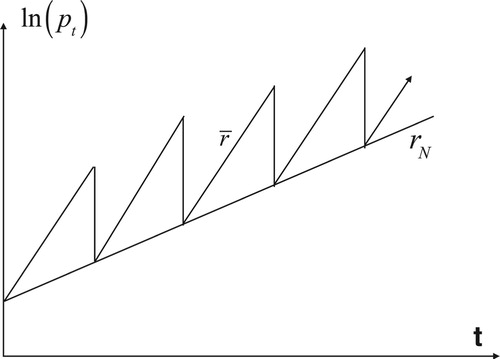
Figure B1. Schematic representation of the price process, which grows instantaneously at the growth rate $\overline{r}>r_N$ and crashes periodically with an amplitude k $\ln (p_t/\exp (r_{N}t\left)\right)$ proportional with a coefficient k ≤ 1 to the mispricing with respect to the average fundamental price process with return $r_N$. This “efficient crash” condition ensures that the long-term growth is given by $r_N$.

In terms of $X_t:=\ln \left(p_t\right)$ and $Y_t:=\ln \left(p_t^N\right)$ and, changing the time scale in units of T, so that t = 0, T, 2 T, 3 T, … corresponds to t = 0, 1, 2, 3, … , this model can be written as follows: (B1) $X_{t+1}=X_t+\overline{r}T-k\left(X_t-Y_t\right)$(B1) (B2) $Y_{t+1}=Y_t+r_{N}T$(B2) This yields (B3) $X_{t+1}=(1-k)X_t+\overline{r}T+k\left(r_{N}T\right)t$(B3) (B4) $Y_t=\left(r_{N}T\right)t$(B4)

Expression (B4) is the trivial recovery that the log-price of the normal process increases by $r_{N}T$ over each period T.

For perfectly “efficient” crashes that bring back regularly the price at exactly the normal price at the instants nT, n = 1, 2, … , the coefficient k is then exactly equal to 1. For k = 1, expression (B3) simplifies to $X_t=\overline{r}T+\left(r_{N}T\right)t$, which grows with the normal price at the same growth rate r_N, up to a translation due to the transient from time 0 to T.

For k < 1, the solution is less obvious and needs a more careful examination. The series (B3) can be solved using the formalism of generating probability function (GPF). Let us consider the general equation (B5) $X_t=a{X}_{t-1}+\alpha t+\beta .$(B5)

We thus have a = 1−k, $\beta =\overline{r}T$ and $\alpha =k\left(r_{N}T\right)$.

We introduce the GPF (B6) $P\left(z\right)=\sum _{t=0}^{\mathrm{\infty }}{X}_t{z}^t,$(B6) Multiplying (B5) by z^t and summing over t leads after some simple summations of series to the equation for P(z): (B7) $P\left(z\right)=X_0+azP\left(z\right)+\frac{\alpha z}{{(1-z)}^2}+\frac{\beta z}{1-z},$(B7) whose solution is obviously (B8) $P\left(z\right)=\frac{X_0}{1-az}+\frac{\alpha z}{(1-az){(1-z)}^2}+\frac{\beta z}{(1-az)(1-z)},$(B8) Expanding the r.h.s. of expression (B8) in series of integer powers of z and identifying term by term with the definition (B6) leads to the general solution: (B9) $X_t=X_0{a}^t+\alpha \frac{t(1-a)-a+a^{t+1}}{{(1-a)}^2}+\beta \frac{1-a^t}{1-a}.$(B9) Let us take 0 < k < 1, then 0 < a = 1−k < 1 so that $a^t$ converges to 0 exponentially fast. Thus, at long times, (B9) reduces with an excellent approximation to (B10) $X_t=\alpha \frac{t(1-a)-a}{{(1-a)}^2}+\beta \frac{1}{1-a}.$(B10) This solution (B10) can be checked by replacing directly in equation (B5). One can also use a simpler route than the full generating probability function formalism, which consists in searching for a solution of the form $X_t=mt+b$. Replacing in (B5) yields m = α/(1−a) and b = β/(1−a) – aα(1−a)², which recovers the exact (B10). One should note that this linear ansatz provides only the asymptotic shape of the solution, while the generating probability function formalism gives additionally the structure of the transient dynamics stemming from the initial condition.

The return of the price is asymptotically given by $\frac{1}{t}{X}_t$ which yields (B11) $\underset{t\to \mathrm{\infty }}{lim}\frac{1}{t}\ln \left(p_t\right):=\underset{t\to \mathrm{\infty }}{lim}\frac{1}{t}{X}_t=\alpha \frac{1}{1-a}.$(B11)

With a = 1−k and $\alpha =k\left(r_{N}T\right)$, this yields that the long-term average return is equal to $r_{N}T$ when time is counted discretely in units of T. Thus, notwithstanding the fact that the crash is only a fraction k < 1 of the bubble size $\ln (p_t/\exp (r_{N}t\left)\right)$, the long-term average return of the periodically collapsing price is equal to the return $r_N$ of the normal price. In other words, the price of the risky asset grows at the same long-term growth rate as the smooth normal price, even if it grows instantaneously as the faster rate $\overline{r}>r_N$.

Appendix C

Proposition C.3:

$L\left(\lambda \right)$ is defined and there exits ${\lambda }_t^A$ and ${\lambda }_t^B$ such that it is a strictly concave function of $\lambda \in \mathrm{\Omega }$ with $\mathrm{\Omega }=\left\{\lambda |{\lambda }_t^A\le \lambda \le {\lambda }_t^B\text{ with }{\lambda }_t^L\le {\lambda }_t^A<0<{\lambda }_t^B\le {\lambda }_t^U\right\}$ provided $\sigma >0$ or if $\rho \ne 0$ and either $\overline{r}-r_f+{\sigma }^2/2\ne 0$ or $\overline{\text{K}}\ln \left(q_t\right)+r_D-r_f+{\sigma }^2/2\ne 0$.

Proof:

As in (14), we split $L\left(\lambda \right)$ (dropping the t subscript on $\lambda$), into two terms and consider the first term (C1) $\begin{array}{r}\begin{array}{rl}{L}_1\left(\lambda \right)& =2\ln \left[e^{r_f}\left(1+\lambda \left(e^z-1\right)\right)\right]-\frac{1}{2}\ln \left(e^{2r_f}\left[{\left(1+\lambda \left(e^z-1\right)\right)}^2+{\lambda }_{}^2{e}^{2z}\left(e^{{\sigma }^2}-1\right)\right]\right)\\ & =r_f+2\ln \left[1+\lambda \left(e^z-1\right)\right]-\frac{1}{2}\ln \left({\left(1+\lambda \left(e^z-1\right)\right)}^2+{\lambda }_{}^2{e}^{2z}\left(e^{{\sigma }^2}-1\right)\right)\\ & \text{with }z=\overline{r}-r_f+\frac{{\sigma }^2}{2}\end{array}\end{array}$(C1)

Then we have: (C2) $\frac{\mathrm{\partial }{L}_1}{\mathrm{\partial }\lambda }=\frac{2\left(e^z-1\right)}{1+\lambda \left(e^z-1\right)}-\frac{\left(1+\lambda \left(e^z-1\right)\right)\left(e^z-1\right)+\lambda e^{2z}\left(e^{{\sigma }^2}-1\right)}{{\left(1+\lambda \left(e^z-1\right)\right)}^2+{\lambda }^2{e}^{2z}\left(e^{{\sigma }^2}-1\right)}$(C2) And (C3) $\begin{array}{r}\begin{array}{rl}\frac{{\mathrm{\partial }}^2{L}_1}{\mathrm{\partial }{\lambda }^2}& =-2\frac{{\left(e^z-1\right)}^2}{{\left(1+\lambda \left(e^z-1\right)\right)}^2}\\ & -\frac{\left[{\left(1+\lambda \left(e^z-1\right)\right)}^2+{\lambda }^2{e}^{2z}\left(e^{{\sigma }^2}-1\right)\right]\left[{\left(e^z-1\right)}^2+e^{2z}\left(e^{{\sigma }^2}-1\right)\right]}{{\left[{\left(1+\lambda \left(e^z-1\right)\right)}^2+{\lambda }^2{e}^{2z}\left(e^{{\sigma }^2}-1\right)\right]}^2}\\ & +\frac{\left[\left(1+\lambda \left(e^z-1\right)\right)\left(e^z-1\right)+\lambda e^{2z}\left(e^{{\sigma }^2}-1\right)\right]\left[2\left(1+\lambda \left(e^z-1\right)\right)\left(e^z-1\right)+2\lambda e^{2z}\left(e^{{\sigma }^2}-1\right)\right]}{{\left[{\left(1+\lambda \left(e^z-1\right)\right)}^2+{\lambda }^2{e}^{2z}\left(e^{{\sigma }^2}-1\right)\right]}^2}\end{array}\end{array}$(C3) Thusly $\begin{array}{rl}& L_1\left(0\right)=r_f\\ & {\left.\frac{\mathrm{\partial }{L}_1}{\mathrm{\partial }\lambda }\right|}_{\lambda =0}=e^z-1\\ & {\left.\frac{{\mathrm{\partial }}^2{L}_1}{\mathrm{\partial }{\lambda }^2}\right|}_{\lambda =0}=-(e^z-1{)}^2-e^{2z}\left(e^{{\sigma }^2}-1\right)\end{array}$And we have for $L\left(\lambda \right)$ that $\begin{array}{rl}& L\left(0\right)=r_f\\ & {\left.\frac{\mathrm{\partial }L}{\mathrm{\partial }\lambda }\right|}_{\lambda =0}=\left(1-\rho \right)e^z+\rho e^z-1\\ & {\left.\frac{{\mathrm{\partial }}^{2}L}{\mathrm{\partial }{\lambda }^2}\right|}_{\lambda =0}=-\left(1-\rho \right)\left[{\left(\exp \left({\overline{r}}_t+\frac{{\sigma }^2}{2}\right)-1\right)}^2+\exp \left(2{\overline{r}}_t+{\sigma }^2\right)\left(e^{{\sigma }^2}-1\right)\right]\\ & -\rho \left[{\left(\exp \left({\kappa }_i\ln \left(q_t\right)+r_D+\frac{{\sigma }^2}{2}\right)-1\right)}^2+\exp \left(2{\kappa }_i\ln \left(q_t\right)+2r_D+{\sigma }^2\right)\left(e^{{\sigma }^2}-1\right)\right]\end{array}$QED

Appendix D

Proposition D.4:

We can approximate an optimal ${\lambda }_t^{\ast }$ by

$\begin{array}{rl}& {\lambda }^{\ast }\approx \frac{\tilde{D}-1+\frac{\tilde{D}{\sigma }^2}{2}}{\left(1-\rho \right){\left(\tilde{A}-1\right)}^2+\rho {\left(\tilde{B}-1\right)}^2+H_2+H_3}\\ & \text{with}\\ & \tilde{A}\equiv \exp \left(\overline{r}-r_f\right)\\ & \tilde{B}\equiv \exp \left(\overline{K}\ln \left(q_t\right)+r_D-r_f\right)\\ & \tilde{D}\equiv \left(1-\rho \right)\tilde{A}+\rho \tilde{B}\\ & H_2=\left(2\left(\left(1-\rho \right){\tilde{A}}^2+\rho {\tilde{B}}^2\right)-\tilde{D}\right){\sigma }^2\\ & H_3=\left(\left(1-\rho \right){\tilde{A}}^2+\rho {\tilde{B}}^2\right)\frac{3{\sigma }^4}{4}\end{array}$We can further approximate $\tilde{A}$, $\tilde{B}$, and $\tilde{D}$ by $\tilde{A}\approx 1+\overline{r}-r_f$, $\tilde{B}=1+\overline{K}\ln \left(q_t\right)+r_D-r_f$, and $\tilde{D}\approx 1+r_D-r_f$ so that we have using $2\left(\left(1-\rho \right){\tilde{A}}^2+\rho {\tilde{B}}^2\right)-\tilde{D}\approx 1+3\left(\overline{r}-r_f+\overline{K}\ln \left(q_t\right)+r_D-r_f\right)$ that yields ${\lambda }^{\ast }\approx \frac{r_D-r_f+{\sigma }^2/2}{{\sigma }^2+\left(1-\rho \right){\left(\overline{r}-r_f\right)}^2+\rho {\left(\overline{K}\ln \left(q_t\right)+r_D-r_f\right)}^2}$

Proof:

From (9) and (10), we have: (D1) $\begin{array}{r}\begin{array}{rl}L\left({\lambda }_t\right)& \equiv E\left[\ln \left(\frac{w_{t+1}}{w_t}\right)\right]=E\left[\ln \left(\exp \left(r_f\right)\left(1+{\lambda }_t\left(\exp \left({\overline{a}}_t+\sigma {\epsilon }_t\right)-1\right)\right)\right)\right]\\ & =\frac{1-\rho }{\sqrt{2\pi }}\underset{-\mathrm{\infty }}{\overset{+\mathrm{\infty }}{\int }}\left[\ln \left(\exp \left(r_f\right)\left[1+{\lambda }_t\left(\tilde{A}\exp \left(\sigma \epsilon \right)-1\right)\right]\right)\right]\exp \left(-\frac{{\epsilon }^2}{2}\right)d\epsilon \\ & +\frac{\rho }{\sqrt{2\pi }}\underset{-\mathrm{\infty }}{\overset{+\mathrm{\infty }}{\int }}\left[\ln \left(\exp \left(r_f\right)\left[1+{\lambda }_t\left(\tilde{B}\exp \left(\sigma \epsilon \right)-1\right)\right]\right)\right]\exp \left(-\frac{{\epsilon }^2}{2}\right)d\epsilon \end{array}\end{array}$(D1) And by the RE condition: (D2) $\tilde{D}\approx 1+r_D-r_f$(D2) As ${\overline{r}}_t$ can be large, we use the following second order expansions for log and exponential: (D3) $\begin{array}{r}\begin{array}{rl}& \ln \left(x\right)\approx \left(x-1\right)-\frac{1}{2}(x-1{)}^2|x-1|\le 1,x\ne 0\\ & \exp \left(x\right)\approx 1+x+\frac{x^2}{2}\end{array}\end{array}$(D3) Because of (13), the log arguments are bounded away from zero, and then the expressions (12) becomes: (D4) $\begin{array}{r}\begin{array}{rl}E\left[\ln \left(\frac{w_{t+1}}{w_t}\right)\right]& \approx \frac{1-\rho }{\sqrt{2\pi }}\underset{-\mathrm{\infty }}{\overset{+\mathrm{\infty }}{\int }}\left[\ln \left({\lambda }_t\left(\tilde{A}\left(1+\sigma \epsilon +\frac{{\sigma }^2{\epsilon }^2}{2}\right)-1\right)+1\right)\right]\exp \left(-\frac{{\epsilon }^2}{2}\right)d\epsilon \\ & +\frac{\rho }{\sqrt{2\pi }}\underset{-\mathrm{\infty }}{\overset{+\mathrm{\infty }}{\int }}\left[\ln \left({\lambda }_t\left(\tilde{B}\left(1+\sigma \epsilon +\frac{{\sigma }^2{\epsilon }^2}{2}\right)-1\right)+1\right)\right]\exp \left(-\frac{{\epsilon }^2}{2}\right)d\epsilon \\ & +r_f\end{array}\end{array}$(D4) We expand the integrand using: (D5) $\frac{1}{\sqrt{2\pi }}\underset{-\mathrm{\infty }}{\overset{+\mathrm{\infty }}{\int }}{\epsilon }^m\exp \left(-\frac{{\epsilon }^2}{2}\right)d\epsilon =\left\{\begin{array}{c}0m\text{odd}\\ 2^{-m/2}\frac{m!}{\left(m/2\right)!}m\text{even}\end{array}\right.$(D5) which gives for the first integrand: (D6) $\begin{array}{r}\begin{array}{rl}& \frac{1}{\sqrt{2\pi }}\underset{-\mathrm{\infty }}{\overset{+\mathrm{\infty }}{\int }}\left[\ln \left({\lambda }_t\left(\tilde{A}\left(1+\sigma \epsilon +\frac{{\sigma }^2{\epsilon }^2}{2}\right)-1\right)+1\right)\right]\exp \left(-\frac{{\epsilon }^2}{2}\right)d\epsilon \\ & =\frac{1}{\sqrt{2\pi }}\underset{-\mathrm{\infty }}{\overset{+\mathrm{\infty }}{\int }}\left[{\lambda }_t\left(\tilde{A}\left(1+\sigma \epsilon +\frac{{\sigma }^2{\epsilon }^2}{2}\right)-1\right)-\frac{1}{2}{\lambda }_t^2{\left(\tilde{A}\left(1+\sigma \epsilon +\frac{{\sigma }^2{\epsilon }^2}{2}\right)-1\right)}^2\right]\exp \left(-\frac{{\epsilon }^2}{2}\right)d\epsilon \\ & \approx \end{array}\end{array}$(D6) Expanding the first integrand and dropping the subscript t gives: (D7) $\begin{array}{r}\begin{array}{rl}& \ln \left(\lambda \left(\tilde{A}\left(1+\sigma \epsilon +\frac{{\sigma }^2{\epsilon }^2}{2}\right)-1\right)+1\right)\\ & \approx \lambda \left(\tilde{A}\left(1+\sigma \epsilon +\frac{{\sigma }^2{\epsilon }^2}{2}\right)-1\right)-\frac{1}{2}{\lambda }^2{\left(\tilde{A}\left(1+\sigma \epsilon +\frac{{\sigma }^2{\epsilon }^2}{2}\right)-1\right)}^2\\ & =\lambda \left(\tilde{A}-1\right)-\frac{1}{2}{\lambda }^2\left(1-2\tilde{A}+{\tilde{A}}^2\right)\\ & +\epsilon \left(\lambda \tilde{A}\sigma -\frac{1}{2}{\lambda }^2\left(2\sigma {\tilde{A}}^2-2\tilde{A}\sigma \right)\right)\\ & +{\epsilon }^2\left(\lambda \tilde{A}\frac{{\sigma }^2}{2}-\frac{1}{2}{\lambda }^2\left(-\tilde{A}{\sigma }^2+2{\sigma }^2{\tilde{A}}^2\right)\right)\\ & +{\epsilon }^3\left(-\frac{1}{2}{\lambda }^2\left({\sigma }^3{\tilde{A}}^2\right)\right)\\ & +{\epsilon }^4\left(-\frac{1}{2}{\lambda }^2\left(\frac{{\sigma }^4{\tilde{A}}^2}{4}\right)\right)\end{array}\end{array}$(D7) Therefore, the first integrand is given by: (D8) $\begin{array}{r}\begin{array}{r}\lambda \left(\tilde{A}-1+\tilde{A}\frac{{\sigma }^2}{2}\right)\\ & -\frac{1}{2}{\lambda }^2\left(1-2\tilde{A}+{\tilde{A}}^2-\tilde{A}{\sigma }^2+2{\sigma }^2{\tilde{A}}^2+\frac{3{\sigma }^4{\tilde{A}}^2}{8}\right)\end{array}\end{array}$(D8) The second integrand is of the same form so that we have: (D9) $\begin{array}{r}\begin{array}{rl}\frac{\mathrm{\partial }L\left(\lambda \right)}{\mathrm{\partial }\lambda }\approx & \left(1-\rho \right)\left[\tilde{A}-1+\frac{\tilde{A}{\sigma }^2}{2}-\lambda \left({\sigma }^2\left(2{\tilde{A}}^2-\tilde{A}\right)+{\left(\tilde{A}-1\right)}^2+\frac{3{\tilde{A}}^2{\sigma }^4}{4}\right)\right]\\ & +\rho \left[\tilde{B}-1+\frac{\tilde{B}{\sigma }^2}{2}-\lambda \left({\sigma }^2\left(2{\tilde{B}}^2-\tilde{B}\right)+{\left(\tilde{B}-1\right)}^2+\frac{3{\tilde{B}}^2{\sigma }^4}{4}\right)\right]\\ & =\tilde{D}\left(1+\frac{{\sigma }^2}{2}\right)-1-\lambda \left(\begin{array}{c}\left(1-\rho \right)(\tilde{A}-1{)}^2+\rho (\tilde{B}-1{)}^2\\ +\left(\left(\left(1-\rho \right)2{\tilde{A}}^2+2\rho {\tilde{B}}^2\right)-\tilde{D}\right){\sigma }^2\\ +\left(\left(1-\rho \right){\tilde{A}}^2+\rho {\tilde{B}}^2\right)\frac{3{\sigma }^4}{4}\end{array}\right)\end{array}\end{array}$(D9) Note that $\tilde{D}\left(1+{\sigma }^2/2\right)-1\approx r_D-r_f+{\sigma }^2/2$

The approximation is a strictly concave function if $\left(1-\rho \right)(\tilde{A}-1{)}^2+\rho (\tilde{B}-1{)}^2+H_2+H_3>0$. Assuming this to be the case, we set $\mathrm{\partial }\overline{E}\left(\lambda \right)/\mathrm{\partial }\lambda =0$ and calculate: (D10) ${\lambda }^{\ast }=\frac{\tilde{D}\left(1+\frac{{\sigma }^2}{2}\right)-1}{\left(1-\rho \right){\left(\tilde{A}-1\right)}^2+\rho {\left(\tilde{B}-1\right)}^2+H_2+H_3}$(D10)

Notes

1 This is not to be confused with the interest rate charged to commercial banks by the Federal Reserve, although it could refer to that.

2 We call it the ‘normal price return’. Some may interpret this as a fundamental price return but that is not the specific intention here.

3 We use 60 days based on testing giving reasonable results.

4 Both papers are essentially about gambling and both can also be found in MacLean, Thorp, and Ziemba (2010). Kelly had originally titled the paper ‘Information Theory and Gambling’ but this was nixed by executives as they thought it would reflect poorly on Bell labs.

5 There is a debate on whether to include risks in the objective or as separate risk constraints. One of the authors tends toward the second method and explains why in (Kreuser 2014).

6 See for example optimizers linked to GAMS https://www.gams.com/. Alternatively, we could apply Golden Section search in this one-dimensional search since the function is concave.

7 See Thorp (2006, 2010) for more on the Kelly criterion.

8 The compound annualized growth rate.

9 The CAGR divided by the maximum drawdown (Young 1991).