Quantifying endogeneity of cryptocurrency markets

Abstract

We construct a ‘reflexivity’ index to measure the activity generated endogenously within a market for cryptocurrencies. For this purpose, we fit a univariate self-exciting Hawkes process with two classes of parametric kernels to high-frequency trading data. A parsimonious model of both endogenous and exogenous dynamics enables a direct comparison with exchanges for traditional asset classes, in terms of identified branching ratios. We also formulate a ‘Hawkes disorder problem,’ as generalization of the established Poisson disorder problem, and provide a simulation-based approach to determining an optimal observation horizon. Our analysis suggests that Bitcoin mid-price dynamics feature long-memory properties, well explained by the power-law kernel, at a level of criticality similar to fiat-currency markets.

Keywords:

• Bitcoin
• branching ratio
• cryptocurrencies
• endogeneity
• Hawkes process
• market reflexivity
• trading behavior

1. Introduction

Bitcoin, introduced by Nakamoto (2008), is arguably one of the most interesting financial innovations of this century. Without any central authority an ad hoc peer-to-peer network issues a tradeable asset that can be considered an alternative to fiat currencies, with all the necessary features such as value storage and fungibility (as a medium of exchange). Moreover, cryptocurrencies offer certain advantages, such as fast and low-cost execution – particularly when compared to traditional financial institutions. The underlying blockchain technology renders the recorded transactions public and transparent. Meanwhile, the cryptocurrency space has spawned thousands of Bitcoin-like digital assets, creating a financial platform akin to foreign-exchange markets for fiat currencies. Yet, with a market capitalization of about $200 billion its size is still fairly insignificant in comparison with the $20 trillion invested in the S&P 500 stock index. Current public discussion tends to focus on certain technical or legal points. Regarding the place of Bitcoin in the current financial system, Baur, Hong, and Lee (2018) conclude that Bitcoin is a speculative asset and thus far has not served as an alternative currency or medium of exchange. Kristoufek (2015) – using a wavelet analysis – recognizes Bitcoin as a hybrid asset whose price is influenced by money supply and adoption in trade, quite in accordance with standard economic theory. As of now, our understanding of cryptocurrencies and their place within the traditional monetary system remains sketchy. Despite the fact that crypto-market capitalization has grown significantly, the market itself has been almost entirely unregulated. The lack of a centralized regulatory body, together with extreme market swings, has given rise to much criticism and caution. On the other hand, the apparently functioning crypto-market presents a natural experiment introducing one of the most laissez-faire financial exchanges of all time, which invites research on market dynamics and investment behavior. Indeed, cryptocurrency exchanges offer unprecedented public access to market data, thus allowing for in-depth analyses and comparisons to the theory describing their traditional counterparts.

Conceptually, one can think of financial markets as devices to convert information and beliefs about underlying fundamentals into prices (Grossman 1989). A critical question, that still remains largely unanswered (not only for cryptocurrencies), is how much prices are indeed driven by observable information. In other words, are markets sufficiently immediate and efficient to track rapid changes of security valuations with commensurate price adjustments? According to the strong version of the Efficient Market Hypothesis (EMH), prices are a perfect reflection of available news (Fama 1970). That is, markets are driven exogenously:¹ any new information is instantaneously absorbed and reflected in a new equilibrium price. If this is the case (and investors are rational), a market crash can arise only as a consequence of a negative high-impact news release or when significant indicator thresholds are crossed (Reinhard and Rogoff 2009). However, global financial markets have witnessed multiple flash-crash events in which vast amounts of capital were lost and again recovered in a matter of minutes, without any clear exogenous trigger. Using high-frequency data, Bouchaud (2009) concludes that merely a small fraction of significant price jumps can be explained by exogenous events. Furthermore, empirical anomalies do not conform with the neoclassical framework, such as the ‘excess volatility puzzle’ where prices move more than would be justified by the pertinent news flows (LeRoy and Porter 1981; Shiller 1981). Even in the cryptocurrency research community the EMH has been a source of persistent controversy. For instance, Kristoufek (2018) and Urquhart (2016) conclude that Bitcoin markets are close-to-efficient. By contrast, Jiang, Nie, and Ruan (2018), as well as Vidal-Tomás, Ibáñez, and Farinós (2019), obtain empirical results which tend to contradict the EMH. The latter evidence suggests the presence of a significant endogenous component, especially on smaller timescales, critical for the price evolution of digital currencies. Thus, one expects that overall price dynamics must be driven by a time-dependent complex interplay of exogenous and endogenous factors. Collective behavioral phenomena, such as herding or imitation (Hong, Kubik, and Stein 2005; Lux 1995), offer some plausible explanations. Indeed, Bouri, Gupta, and Roubaud (2019) and Ajaz and Kumar (2018) provide empirical evidence for herding behavior in cryptocurrency markets. However, their respective methodologies – based on cross-sectional standard deviations of daily returns – are impervious to the more granular intra-day trading events. Additional sources of the unexplained endogeneity are frequently attributed to strategic order splitting, margin calls, stop-loss triggers, or high-frequency traders.

Recently, a class of self-exciting point processes was recognized as a suitable tool for disentangling and quantifying the underlying dynamics of the price process, as one of its inherent features is a neat separation of the endogenous and exogenous action triggers. The discussion on endogeneity and its evolution in the markets (i.e., the endo-exo problem) was broached by Filimonov and Sornette (2012), who fit a univariate exponential Hawkes process to E-mini S&P 500 futures traded between 1998 and 2010. They discuss reflexivity² on a micro-scale (i.e., in intervals of less than 1 hour) and report a significant increase in the level of endogeneity over the observed period (from 0.3 in 1998 to 0.8 in 2012), which can be attributed to the rise in algorithmic trading. Hardiman, Bercot, and Bouchaud (2013) (‘HBB’) revisit this problem with the same dataset; however, instead of the fast decaying exponential, they opt for a heavy-tail long-memory power-law kernel. While agreeing about the rise in the short-term reflexivity, the authors conclude that markets were in fact persistently operating around the criticality level. Their corollary is that price dynamics are therefore best described by two separate kernels, for long- and short-term memory – thus taking into account the meso market structure (in intervals of about 1 day). This argument has been further elaborated by other researchers. Filimonov et al. (2014) identify numerous estimation-related issues in HBB's methodology, such as an upward bias in the presence of outliers for the power-law kernel norm, whence questioning HBB's results. To settle the discussion Hardiman and Bouchaud (2014) develop an empirical estimator of the branching ratio, further supporting their claims of market criticality and the presence of long-memory properties.

Despite cryptocurrencies being an active field of research, to the best of our knowledge, as of yet there has been no discussion on the origins of price dynamics. In this paper, we quantify the degree of market endogeneity and investigate its temporal dependence. This allows us to estimate the market susceptibility (and inefficiency due) to endogenous behavioral biases (such as herding) as well as its reactiveness to exogenous shocks. We also uncover structural similarities in the price dynamics of cryptocurrencies, equities, commodities, and foreign exchange (FX) markets. The findings shed light on the nature of Bitcoin from the vantage point of self-exciting point processes.

Our paper proceeds as follows. Section 2 motivates and introduces the Hawkes model along with its branching-structure representation which allows us to characterize the endo-exo dynamics. Section 3 follows with a description of the dataset. Section 4 presents the key findings, and Section 5 concludes.

2. Model

2.1. Motivation

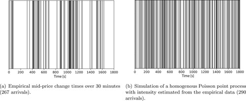
Before diving into the methodology of self-exciting point processes, it is useful to pinpoint the salient deficiencies of standard models which do not capture the endogenous component in the price dynamics. Consider a sequence of trade times $({\tau }_1,{\tau }_2,\dots )$, observed over the time interval [0, T] for some observation horizon $T>0$. Disregarding the direction and volume of the trades, and assuming independence among them (i.e., every trader acts independently based on private information), this description corresponds to a perfectly exogenous market without behavioral biases such as imitation or herding. Therefore, for sufficiently small time intervals (to account for intra-day structural breaks) the observed order arrivals should reasonably well follow a homogenous Poisson point process (HPP). Figure 1 shows an empirical realization of trade arrivals (in a 30-minute window), next to a simulated sequence of Poisson arrivals at the same rate. It can be easily seen that an HPP does not capture the essence of the empirical sequence, since observed market orders exhibit marked clustering – quite in contrast to a memoryless Poisson process.³

Figure 1. Barcode plots.

A natural extension of an HPP is a Markov-modulated Poisson process (MMPP), as an instance of a ‘hidden Markov model.’ An MMPP is a doubly stochastic point process whose intensity depends on the (unobserved) state of a Markov process. MMPPs have been applied successfully to return data in view of identifying structural breaks and distinguishing different volatility regimes (Engel 1994). However, when setting up an MMPP, a critical decision has to be made at the model-specification stage on the number of hidden states, for example, with help of information criteria. In our dataset, a reliable calibration of an MMPP proved infeasible: our fits indicated an improvement with an increasing number of hidden states (to more than 10) with respect to both AIC and BIC,⁴ suggesting a fragmented process with no clear state separation.

Remark 2.1

Using the CSR (complete spatial randomness) framework described by Clark and Evans (1954) one can strongly reject the null hypothesis of spatial randomness, practically for any time horizon (ranging from mere minutes to full days). This finding is in line with the barcode in Figure 1(a), which features heavy clustering.

2.2. Univariate Hawkes process

A univariate Hawkes process is a linear self-exciting point process with a conditional intensity function, defined as (1) $\lambda \left(t|{\mathcal{H}}_t\right)=\mu \left(t\right)+{\int }_0^{t}g(t-\tau )\mathrm{d}{N}_{\tau }=\mu \left(t\right)+\sum _{i:{\tau }_i<t}g(t-{\tau }_i),t\ge 0,$(1) where ${\tau }_i>0$ denotes the ith arrival time (for $i\ge 1$). The baseline intensity $\mu \left(t\right)$ is a deterministic function of time, while $g:{\mathbb{R}}_{+}\to {\mathbb{R}}_{+}$ is a (nonnegative-valued) self-excitation function (or ‘memory kernel’) which determines the covariance properties of the process. The filtration ${\mathcal{H}}_t$ describes the estimation-relevant record of the process history and for our purposes includes all event-arrival times on the interval $[0,t)$, for $t\ge 0$.

In the framework of Hawkes processes, ‘endogeneity’ refers to the ability of generating new arrivals from past events. This notion of endogeneity can be reinforced and formalized using an alternative but equivalent view of the process in terms of a (stochastic) branching structure (Hawkes and Oakes 1974). The latter provides for a direct mapping between arrivals and clusters, where each cluster starts with an immigrant generated from an inhomogeneous Poisson process with baseline intensity μ. Consistent with Equation (1(1) $\lambda \left(t|{\mathcal{H}}_t\right)=\mu \left(t\right)+{\int }_0^{t}g(t-\tau )\mathrm{d}{N}_{\tau }=\mu \left(t\right)+\sum _{i:{\tau }_i<t}g(t-{\tau }_i),t\ge 0,$(1) ), every arrival triggers a spike in the intensity through the memory kernel, thus generating its own offspring arrivals according to an inhomogeneous Poisson process of intensity g. This cascades through all offsprings, effectively creating a hierarchical branching structure. Eventually, every event can be labeled either as an ‘immigrant,’ generated exogenously through the deterministic drift without an existing parent, or as an endogenously created ‘offspring.’ The central parameter controlling the size of endogenously generated offspring families, generally referred to as the ‘branching ratio’ n, is defined as the average number of offsprings per event: (2) $n={\int }_0^{\mathrm{\infty }}g\left(t\right)\mathrm{d}t.$(2) Conceptually, the branching ratio determines the degree of self-excitation in the process. The latter captures the percentage of the arrivals that are generated endogenously – as a consequence of previous arrivals. Based on the value of the branching ratio, one can distinguish four different regimes:

1. n = 0 (memoryless): inhomogeneous Poisson point process which features exclusively immigrant arrivals;

2. n<1 (subcritical): nonexplosive process;⁵

3. n = 1 (critical): marginally unstable (or stable) process where a generation of offsprings lives indefinitely (the existence of such processes was proved by Brémaud and Massoulié (2001) for $\mu \left(t\right)=0$);

4. n>1 (supercritical): nonstationary explosive process with finite intensity but infinite/nonintegrable covariance. (In other words, a single event starts an infinite family, and the process explodes.)

This fourfold separation provides a succinct partition for the endo-exo market dynamics, similar in interpretation to such distinctions in the context of well-established autoregressive processes. Ultimately, it allows us to describe the endogeneity by a characteristic number, comparable across asset classes and financial instruments.

When inferring the branching ratio from data one has two main options: either stochastic declustering (Zhuang, Ogata, and Vere-Jones 2002) (which essentially requires reverse-engineering of the clusters) or maximum-likelihood estimation (MLE) in combination with Equation (2(2) $n={\int }_0^{\mathrm{\infty }}g\left(t\right)\mathrm{d}t.$(2) ). In the remainder of the paper, we pursue the second approach for its relative simplicity and clarity.

2.3. Parametric kernels

The two most prominent classes of (parametrized) self-excitation functions are ‘exponential’ and ‘power-law.’

1. Exponential kernel: (3) $g\left(t\right)=\frac{n}{\text{β}}\exp \left[-\frac{t}{\text{β}}\right],t\ge 0,$(3) where $n\ge 0$ denotes the branching ratio and $\text{β}>0$ is the decay parameter. The exponential kernel satisfies the Markov property, rendering it particularly popular. Furthermore, as shown by Ogata (1981), it allows for recursive maximum-likelihood computations which reduce the computational complexity from $\mathcal{O}\left(N_T^2\right)$ to $\mathcal{O}\left(N_T\right)$.

2. Power-law kernel: (4) $g\left(t\right)=\frac{n\epsilon {\tau }_0^{\epsilon }}{(t+{\tau }_0{)}^{1+\epsilon }},t\ge 0,$(4) where $n\ge 0$ denotes the branching ratio; the shift parameter ${\tau }_0>0$ ensures the integrability of the kernel, and $\epsilon >0$ sets the decay speed. This particular form gained its popularity through the epidemic-type aftershock sequence model of earthquake occurrences.⁶ Compared to the exponential kernel, the power-law kernel features a ‘long memory’ (due to its relatively thick tail) that may be better suited for financial markets than the exponential kernel. Additionally, there exist other variations of the power-law kernel that differ in the way the regularization is introduced. The primary reason for using this class of kernels is the fat tail shared by its various members (at least approximately; see Remark 2.2).

Remark 2.2

Applying directly the power-law kernel as specified in Equation (4(4) $g\left(t\right)=\frac{n\epsilon {\tau }_0^{\epsilon }}{(t+{\tau }_0{)}^{1+\epsilon }},t\ge 0,$(4) ) carries a significant computational burden, as Ogata's recursive MLE formulation (Ogata 1978) is not available. In order to expedite the numerics, we consider an approximation constructed from a power-law-weighted sum of exponential kernels (Bochud and Challet 2007), (4') $g\left(t\right)\approx \hat{g}\left(t\right)\equiv \frac{n}{Z}\sum _{k=0}^{M-1}{a}_k^{-(1+\epsilon )}\exp \left[-\frac{t}{a_k}\right],t\ge 0,$(4') where $a_k={\tau }_0{m}^k$. The power-law substitute $\hat{g}:{\mathbb{R}}_{+}\to {\mathbb{R}}_{+}$ is parametrized by the branching ratio n, the tail exponent ϵ, and the shift parameter ${\tau }_0$. The additional tuning parameters m>1 (best chosen not too large to avoid an excessive saw-tooth pattern for small t) and M>1 impact the quality and range of the approximation. This approximation, employed by HBB, captures long-term dependencies while leveraging a recursive formulation of the maximum-likelihood function, resulting in reduced fitting times. In fact, the formulation allows to accurately reproduce a power-law decaying kernel $g\left(t\right)\sim t^{-1-ϵ}$ for ${\tau }_0=a_0\ll t\ll a_{M-1}$ (Bouchaud et al. 2018). The normalization constant Z is chosen such that n is equal to the true branching ratio of the kernel, ${\int }_0^{\mathrm{\infty }}\hat{g}\left(t\right)\mathrm{d}t=n$, i.e., $Z=\sum _{k=0}^{M-1}({\tau }_0{m}^k{)}^{-\epsilon }={\tau }_0^{-\epsilon }(1-m^{-\epsilon M}\left)/\right(1-m^{-\epsilon })$.

In what follows, all references to a power-law kernel refer to the substitute $\hat{g}$ in Equation (4), with tuning-parameter values $(m,M)=(2,10)$. For more discussion about kernel properties and their differences, see the comprehensive review by Bacry, Mastromatteo, and Muzy (2015).

2.4. Goodness-of-fit tests

A standard method for assessing the quality of a point-process fit is the ‘residual analysis,’ which consists of computing the time-deformed series of durations $\{{\xi }_i{\}}_{i=1}^{\mathrm{\infty }}$ using the estimated conditional intensity $\hat{\lambda }\left(s|{\mathcal{H}}_T\right)$,⁷ ${\xi }_i={\int }_{{\tau }_{i-1}}^{{\tau }_i}\hat{\lambda }\left(s|{\mathcal{H}}_T\right)\mathrm{d}s,$ with ${\tau }_0=0$, and then statistically testing it for theoretical properties. In the case where a Hawkes process presents a fairly accurate description of the empirical data, residuals of the interarrival times are independently and identically distributed (i.i.d.) draws from an exponential distribution with parameter $\lambda =1$. We assess three theoretical properties using the standard statistical tests, as follows:

1. Ljung and Box (1978) test (LB) for the absence of autocorrelations to ensure independence of residuals, using up to 20 lags;

2. Kolgomorov-Smirnov test (KS) for the distance between the empirical and the theoretical distribution of the residual process;

3. Engle and Russell (1998) test (ED) for excess dispersion in the residuals.

In our setting, a parametrized model that passes all three tests simultaneously is considered ‘successful’ and therefore designated as a viable explanation of the observed data.

Remark 2.3

Brock-Dechert-Scheinkman (BDS) Independence Test

The triade of statistical tests (A), (B) and (C) constitutes quite a standard testing suite for Hawkes-process residuals. For the sake of robustness, we performed an additional BDS test of independence (Brock et al. 1996). Given that this additional test did not change the test-survival statistics by much, we argue that a check of the independence hypothesis can be captured satisfactorily by the LB autocorrelation test.

3. Data

Our data set includes all executed transactions on the BitMEX cryptocurrency exchange between March 1 and May 1 of 2019. BitMEX was selected as the largest crypto-exchange in terms of its trading volume, particularly with respect to Bitcoin (BTC) contracts settled in USD. The trading is open 24 hours a day, so that it closely resembles traditional FX markets. Each trade is recorded with its corresponding time stamp, volume, price, and whether or not the transaction changed the last transaction price (resulting in an uptick or downtick). The available millisecond resolution in the data presents the highest available granularity for this market (Table 1).

Table 1. Description of the market-order data from the BitMEX exchange, which accounts for about 10 percent of the entire BTC trading volume.

timestamp	ordertype	volume	price	ticktype	arrival
2019-02-02 22:45:58.560	Buy	20	3433.5	PlusTick	0.000
2019-02-02 22:46:03.493	Sell	10	3433.0	MinusTick	4.933
2019-02-02 22:46:06.754	Sell	50	3433.0	ZeroMinusTick	8.194
2019-02-02 22:46:09.639	Sell	4	3433.0	ZeroMinusTick	11.079
2019-02-02 22:46:10.679	Buy	21	3433.5	PlusTick	12.119

NB. ‘PlusTick’ and ‘MinusTick’ correspond to a recorded uptick and downtick, respectively; ‘ZeroMinusTick’ records a constant price together with the sign of the last nonzero price.

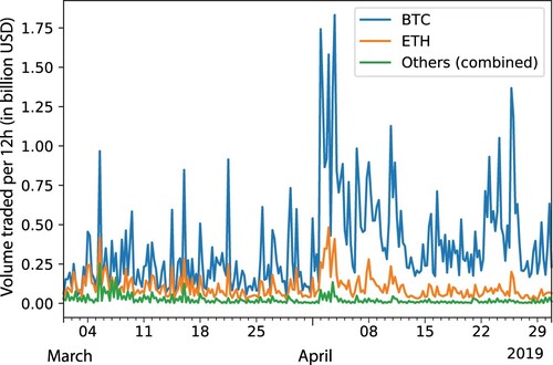
Even though our dataset tracks all BitMEX-traded instruments, including exotics such as Cardano (ADA) or Tron (TRX), we restrict attention to Bitcoin contracts (ticker XBTUSD), since it accounts for the vast majority of trading volume; see Figure 2.⁸

Figure 2. On any given day, the number of transactions (modelled as Hawkes-process arrivals) differs greatly among currencies. Bitcoin contracts account for almost two thirds of the trading activity, and together with the Ethereum market, it accounts for practically all trades. The average number of arrivals on the XBTUSD market is almost an order of magnitude larger than for other currencies, with a peak daily activity of around 1 million recorded trades.

3.1. Measures of market activity

The precise definition of the ‘events’ to be considered is not only critical for the ex-post confidence in the identification of the arrival process, but also for the informational value the estimated coefficients may carry. It is therefore imperative to select a reliable measure of market activity which is robust to the ‘microstructure noise’ omnipresent in high-frequency data. In the finance literature thus far, Hawkes processes have been fitted mainly to the most granular (and noisy) trade data or to various ‘price actions’ (i.e., movements) near the ‘best prices’ (i.e., $a\left(t\right)$ or $b\left(t\right)$; see below). Although the trade-arrival rate may, at first glance, seem to be a reasonable metric for market activity, it does come with an important drawback, as not all trades are equal in their impact due to their quite disparate volumes. To take trade sizes into account, one would need to consider a ‘marked’ version of a Hawkes process which is significantly more intricate to fit.⁹ Practitioners commonly track four different quotations (as a function of time t), each giving rise to a price action and serving a different purpose:

• best-bid $b\left(t\right)$;

• best-ask $a\left(t\right)$;

• last transaction price $p_{\text{tr}}\left(t\right)$;

• mid-price $p_m=\left(a\right(t)+b(t\left)\right)/2$.

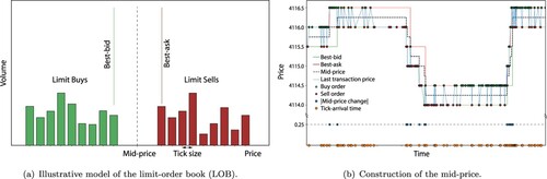
Best-bid and best-ask reflect the upper and lower price boundaries of the standing limit orders (Figure 3(a)), at which a trader can immediately engage in selling or buying (with a market order), respectively, up to the cumulative volume of standing orders in the limit-order book (LOB) at the given price level. They can be regarded as proxies for the market makers' supply and demand.

Figure 3. Limit-order book (a) and construction of the mid-price from transactional data (b).

3.2. Mid-price tracking

When a buy (resp., sell) market order arrives on an exchange at time t, it is paired with the best-ask (resp., best-bid) price available, completing a trade that produces a last transaction price $p_{\text{ tr}}\left(t\right)$. As trades arrive in random order, with the direction of the trade being a random variable as well, the last transaction price jumps sporadically – at times even without concomitant change in supply or demand. This behavior is referred to as ‘bid-ask bounce,’ and it has been established as a proper noise source in its own right (Aït-Sahalia and Yu 2008; Black 1986). Hence, the mid-price is regarded as a more reliable proxy for asset values than the aforementioned best prices (i.e., $a\left(t\right)$ and $b\left(t\right)$), particularly because it does not suffer from the bid-ask bounce; Figure 3(b) shows that $p_m\left(t\right)$ is much less noisy than $p_{\text{ tr}}\left(t\right)$. A change in mid-price can arise due to one of the following three reasons:

1. Cancellation of an existing limit order at the best-bid/ask price;

2. Submission of a new limit order at a new best-bid/ask price;

3. Depletion of the available LOB volume at the best-bid/ask price by market orders.

Even though causes (I) and (II) result from limit orders submitted by liquidity providers (who want to trade), the publicly visible LOB does not reflect the true supply and demand in the market. This comes as a consequence of market participants' (particularly large liquidity providers') reluctance to disclose private information by openly displaying their intentions and intended future positions. Consequently, in fast markets, such as the Bitcoin exchange considered here, a large portion of canceled orders and new limit orders represent so-called ghost orders (Lewis and Baker 2014) whose main purpose is to pry for private information.¹⁰ Indeed, in our dataset cancelations and limit orders account for about 15% of all mid-price changes. We argue that – unlike the first two – it is cause (III) that principally reflects the actual interaction of supply and demand, and as such it should be considered the most reliable information source.

4. Results

Tracking Bitcoin mid-price changes (caused by filled orders between March 1 and May 1, 2019), we now fit a univariate Hawkes process, defined in Equation (1(1) $\lambda \left(t|{\mathcal{H}}_t\right)=\mu \left(t\right)+{\int }_0^{t}g(t-\tau )\mathrm{d}{N}_{\tau }=\mu \left(t\right)+\sum _{i:{\tau }_i<t}g(t-{\tau }_i),t\ge 0,$(1) ), with exponential and power-law kernels, as in Equations (3(3) $g\left(t\right)=\frac{n}{\text{β}}\exp \left[-\frac{t}{\text{β}}\right],t\ge 0,$(3) ) and (4(4) $g\left(t\right)=\frac{n\epsilon {\tau }_0^{\epsilon }}{(t+{\tau }_0{)}^{1+\epsilon }},t\ge 0,$(4) ′), using maximum-likelihood estimation. MLE is our technique of choice for the identification of Hawkes processes, which amounts to solving the following optimization program: (M) $\begin{array}{ll}\underset{\theta \in \mathrm{\Theta }}{max}& \log \mathcal{L}\left(\theta |{\mathcal{H}}_T\right),\\ \text{subject to}& \theta \ge 0,\end{array}$(M) where θ represents a vector of kernel and base-rate parameters. The likelihood function, derived by Rubin (1972), is asymptotically normal, efficient, and consistent (Ogata 1978). As such, it constitutes a straightforward statistical inference technique for the family of self-exciting point processes. The flipside is that its nonconvexity in the decay parameter (β for the exponential and ϵ for the power-law kernel, respectively), coupled with an extreme flatness of the log-likelihood surface near the optimum (Veen and Schoenberg 2008), makes reliable calibration a challenging task (Mark and Weber 2020). In order to circumvent these problems we solve the optimization program (M) in parallel, for a batch of 500 starting guesses and then single out the estimation result for the parameter vector which attains the highest log-likelihood.

Next, we consider the – from a practitioner's standpoint – important question (neglected in the literature thus far) of how to determine the optimal observation length T for an effective estimation of the point-process model in Equation (1(1) $\lambda \left(t|{\mathcal{H}}_t\right)=\mu \left(t\right)+{\int }_0^{t}g(t-\tau )\mathrm{d}{N}_{\tau }=\mu \left(t\right)+\sum _{i:{\tau }_i<t}g(t-{\tau }_i),t\ge 0,$(1) ). After this, we are ready to construct a reflexivity index for cryptocurrency markets (so as to quantify their endogeneity).

4.1. Optimal estimation horizon

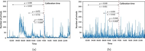
When deliberating about a most preferred observation horizon T, at least for a stationary process with constant parameters a greedy approach (i.e., pursuing ‘more is better’) would indeed appear to be successful. However, in a real-world situation, the empirical trade data at hand most likely would not derive from a single, long, and historically consistent generating process. Thus, a more considerate and appropriate view would be to account for switching regimes, thus allowing conceptually for a data history generated by a concatenation of materially different processes. This problem of detecting the corresponding phase-transition times, commonly known as the Poisson disorder problem (Peskir and Shiryaev 2002), has been studied in the context of homogeneous Poisson processes and unfortunately does not have a straightforward extension to self-exciting processes. Therefore, one has to carefully calibrate the length of the estimation windows such that the history contains a sufficiently large sample for obtaining accurate estimates, while at the same time avoiding a calibration across multiple regimes. On one hand, an inference from a shorter window plays into the assumption of a constant base rate, narrowing the view sufficiently to be able to negate the empirical regularity that mid-price changes feature marked intra-day seasonalities. On the other hand, short estimation windows do limit the kernel's memory and thus disregard interdependencies across time, which develop over hours, days, or even longer periods of time. This interplay of phenomena is illustrated in Figure 4 which compares fits over various observation horizons, for both simulated and empirical data.

Figure 4. Impact of variations in the estimation horizon $T\in \{4,6,12\}$ hours on estimation accuracy. In contrast to simulated data coming from a single point process realization, empirical data features intra-day seasonalities that significantly affect the maximum-likelihood estimates. (a) Empirical data from April 1, 2019. Total number of arrivals: $N_T=30,683$ (for T = 12). (b) Data simulated from an exponential Hawkes process with parameters $\mu =0.05$, $\text{β}=1$ and n = 0.85. Total number of arrivals: $N_T=\text{27,540}$ (for T = 12).

In order to resolve this tradeoff, we rely on a robust numerical experiment. As discussed above, we try to identify a minimal window size T such that the number of observations is sufficient for an ‘accurate’ inference. Consider a family of exponential Hawkes processes with a moderate branching ratio n = 0.5 but variable baseline intensity $\mu \in [0,0.2]$ representing different market regimes.¹¹ We perform an estimation of each process, given observation horizons $T\in [60,10800]$,¹² and we measure the relative estimation error $e=\parallel \hat{\theta }-\theta {\parallel }_2/\parallel \theta {\parallel }_2$, where $\parallel \cdot {\parallel }_2$ denotes the standard Euclidean distance (2-norm). To ensure robustness of the experiment, we obtain a mean relative error for every individual horizon T (using Monte Carlo simulation over 1,000 process realizations). Figure 5(a) depicts the relationship between the observation horizon T and relative error e, obtained as an average across all simulation paths, together with bootstrapped (5%/95%)-confidence intervals (Efron and Tibshirani 1994).

Figure 5. Monte Carlo analysis of the relative error for various baseline regimes. Although Figure 4 was constructed using a fixed branching ratio n = 0.5, the results serve as a conservative decision tool for the optimal horizon $T^{\alpha }$, as higher n-values translate into more observations and thus faster and more reliable calibration. This value for n was not chosen arbitrarily; it is the lowest branching ratio measured on nonoverlapping 10-minute windows using the approximate branching-ratio estimator (Hardiman and Bouchaud 2014). (a) Relative error as a function of the time horizon, for representative base-rate regimes. The red-shaded area represents bootstrapped mean confidence intervals. (b) Relationship between optimal (minimal) observation horizons and different μ-regimes for three representative acceptance thresholds.

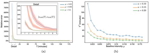
As expected, higher μ-regimes can handle shorter observation horizons – without a significant impact on accuracy. The most preferred (i.e., ‘optimal’) horizon, denoted by $T^{\alpha }$, is selected such that for all $T\ge T^{\alpha }$, it is $e_{0.95}\left(T\right)<\alpha$, where α is a given acceptance threshold.¹³ In other words, the optimal observation horizon is the minimal horizon beyond which the relative error does not exceed α at a 95%-confidence level. Figure 5(b) illustrates the determination of this threshold for various values of μ, resulting in an effective decision tool for determining the optimal observation horizon conditional on a given baseline intensity. More specifically, consider the realization of a self-exciting point process on $[0,T]$, formed as a concatenation of $K\ge 1$ Hawkes processes with different regime parameters $({\mu }_k,n_k)$, for $k\in \{1,\dots ,K\}$, each lasting $T_k$, so $\sum _{k=1}^K{T}_k=T$. The goal is to estimate this process on a rolling horizon, using an observation window of smallest possible length T, so as to prevent averaging the fit over multiple regimes. We approximate the mean intensity $\mathrm{\Lambda }$ of the compound process as follows: (5) $\mathrm{\Lambda }=\sum _{k=1}^K\frac{T_k}{T}{\mathrm{\Lambda }}_k\approx \frac{\mathrm{\#}\text{events on }[0,T]}{T};$(5) using the identity for the average intensity (Hawkes 1971), together with a reasonable upper bound $\overline{n}$ for the branching ratio n. We thus recover (6) $\text{‐}\mu =\mathrm{\Lambda }(1-\overline{\mu }),$(6) which constitutes an approximate lower bound for the baseline mean μ. Together with the downward-sloping dependence of the $T^{\alpha }$ in the baseline intensity $\mu$ (depicted in Figure 5(b) for $\alpha \in \{10\mathrm{\%},15\mathrm{\%},20\mathrm{\%}\}$), the latter yields a minimal observation horizon, which we refer to as ‘optimal estimation horizon’ $T^{\alpha }$, as it most effectively trades off the data requirements for estimation against the volatile nature of regime changes in the trading activity.

Remark 4.1

Although the preceding analysis is purely simulation-based, the results pinpoint high-quality approximations. Indeed, to the best of our knowledge the given simulation-based method provides the first effective work-around for the (as of yet unsolved) ‘Hawkes disorder problem.’ The practical significance of this problem can be gauged by inspecting Figure 9, which shows a typical section of historical price movements and volatility – featuring two distinct regimes of activity. We also note that the estimation results were derived using a Hawkes process with exponential kernel. They readily extend to the power-law formulation in Equation (4), provided that the tail of the kernel does not significantly exceed the observation window.

4.2. Reflexivity index

Building on the analysis from the previous subsection, we now determine the adequate look-back period first by measuring the mean intensity, $\mathrm{\Lambda }=416,019\mathrm{e}\mathrm{v}\mathrm{e}\mathrm{n}\mathrm{t}\mathrm{s}/5,184,000\mathrm{s}=0.08$ events/s. Next, we recover the baseline intensity, $\text{‐}\mu =0.016$ from Equation (6), which corresponds approximately to a 60-minute look-back window (observation horizon T) for a 15% relative error; see Figure 5(b).¹⁴ For direct comparison with the study conducted by Filimonov and Sornette (2012) on S&P 500 E-mini contracts, we calibrate the process for both parametric kernels described in Section 2.3, including the additional look-back periods of 10 and 30 min, on a minute-by-minute rolling horizon.

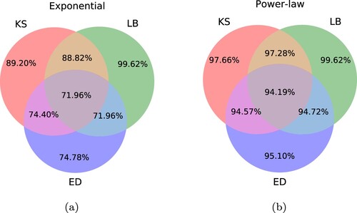
To judge the significance of the results, we refer to Table 2 and Figure 6, which contains pass rates for the statistical tests – together with BIC-values that average across all fits.¹⁵ We observe that with an increasing observation horizon the kernel choice becomes more and more consequential, progressively favoring the power-law variant. Indeed, on the 10-minute timescale the pass rates are almost indistinguishable, with a mild preference for the power-law kernel (based on the BIC value). This is somewhat expected, as a shorter horizon prevents the power-law kernel to leverage its long-memory property; hence, on very short timescales the use of an exponential kernel may well be justified.

Table 2. Fraction of acceptable fits relative to different statistical tests at the 5%-significance level.

	Exponential kernel					Power-law kernel
	KS	LB	ED	KS ∩ LB ∩ ED	Mean BIC	KS	LB	ED	KS ∩ LB ∩ ED	Mean BIC
10 min	99.32%	96.32%	98.10%	93.97%	212.71	99.79%	96.34%	99.70%	95.90%	211.12
30 min	96.44%	98.72%	90.79%	88.03%	583.35	99.19%	98.72%	98.81%	97.23%	576.03
60 min	89.19%	99.61%	74.78%	71.96%	1150.49	97.65%	99.61%	95.09%	94.19%	1131.62

NB. The joint pass rates for a 60-minute estimation window are given in Figure 6. Look-back windows with less than 50 mid-price changes have been excluded.

Figure 6. Fractions of significant fits (in percent) passing the goodness-of-fit criteria. (a) Exponential kernel. (b) Power-law kernel.

The situation dramatically changes for a somewhat larger observation window, of 30-minute length, and a fortiori for a 60-minute observation horizon, where the power-law proves to be a superior choice. This can be deduced from the simultaneous pass with respect to our test triad ($\mathrm{K}\mathrm{S}\cap \mathrm{L}\mathrm{B}\cap \mathrm{E}\mathrm{D}$), and it is further illustrated by Figure 8 which features a quantile-quantile plot of the process residuals for a 60-minute time window, together with the KS p-values for both kernels (calculated as daily averages). A compounding final piece of evidence is given by the empirical distribution of the transformed time series; see Figure 7 – which also shows the Kullback-Leibler divergence for each kernel. Because of its consistent superiority we restrict attention to the power-law kernel.

Figure 7. Comparison of theoretical and empirical densities of transformed interarrival times ${\xi }_i$. The Kullback-Leibler divergence is calculated between the theoretical density $P\sim \mathrm{E}\mathrm{x}\mathrm{p}(\lambda =1)$ and the empirical density of the residuals ${\xi }_i\sim Q$ in Equation (1(1) $\lambda \left(t|{\mathcal{H}}_t\right)=\mu \left(t\right)+{\int }_0^{t}g(t-\tau )\mathrm{d}{N}_{\tau }=\mu \left(t\right)+\sum _{i:{\tau }_i<t}g(t-{\tau }_i),t\ge 0,$(1) ) using the estimator developed by Wang, Kulkarni, and Verdú (2009). (a) Exponential kernel (b) Power-law kernel.

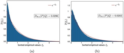
Figure 8. The empirical distribution of transformed arrival times ${\xi }_i$. (a) Q-Q plot of all 60-minute look-back residuals. (b) Average daily p-value of the KS test. The dashed red line represents the 5%-significance level α.

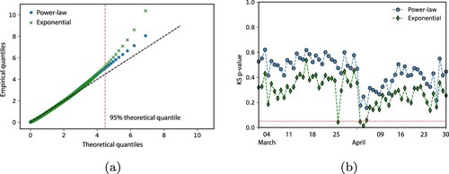
Figure 9. Price and volatility (in USD) in the cryptocurrency market; fluctuations of the baseline intensity (μ); Bitcoin reflexivity index n (in red, for the favored 60-minute interval), computed as a mean of 4-hour windows. The shaded areas bracket the 5%- and 95%-quantiles. [Data for shorter (sub-one-hour) observation horizons are included for comparison with HBB.]

Figure 9 displays the time evolution of the endogenous and exogenous components of the process, and constitutes the Bitcoin reflexivity index for the period. It was obtained from individual fits, so each point represents a 4-hour time period. We observe that the level of endogeneity oscillates around the value n = 0.8 and consistently keeps a significant distance from criticality. This renders Bitcoin comparable to traditional FX markets which exhibit similar values of endogeneity (Lallouache and Challet 2016; Rambaldi, Pennesi, and Lillo 2015). On the other hand, studies on other asset classes report branching ratios strikingly different. For instance, HBB find that futures on equity indices exhibit levels of the branching ratio near criticality, while Filimonov et al. (2014) conclude that within the commodity futures market only around 60% of mid-price changes can be considered endogenous. From the perspective of market microstructure (here: market endogeneity), this suggests that Bitcoin is closer to a fiat currency than gold.¹⁶

Measured levels of endogeneity tend to decrease with longer look-back periods, whereas base-rate estimates go up when increasing the observation horizon. Indeed, by shortening the horizon of the look-back window one tends to ignore events whose impact had not yet fully dissipated. Thus, the estimation (erroneously) credits an excessive portion of the realized intensity to the exogenous component instead of attributing it more correctly to self-excitation. This confirms that even events developed on longer timescales (over tens of minutes and more) play an important role in the microstructure and therefore should not be omitted (e.g., by overly tightening the observation window) – at least in the absence of significant base-rate regime changes.

Lastly, we point out that based on the daily profile of the estimates $\hat{\mu }$ and $\hat{n}$ (Figure 10), the Bitcoin exchange behaves like a true 24/7-market. Again, we emphasize the comparison with FX and equity markets where one clearly observes a ‘lunch lull’ in the form of a U-shaped activity (which requires appropriate corrections in the estimation).

Figure 10. Average number of trade arrivals by time-of-day; average fluctuation of the baseline intensity (μ) by time-of-day; Bitcoin reflexivity index n by time-of-day (in red, for the favored 60-minute interval). The shaded areas represent 5%- and 95%-quantiles. [Daily profile are computed as averages over all significant fits.]

5. Conclusion

We have constructed a reflexivity index for the Bitcoin market that suggests an endogeneity of about 80%. That is, approximately four-fifth of the mid-price changes are determined within the market itself. While this value of the branching ratio is significantly lower than for equity indices (the latter being close to 1), it exceeds the reflexivity of the commodities¹⁷ (such as gold) to which Bitcoin is often compared to. The crypto-market endogeneity corresponds by and large to branching ratios found in FX markets for national currencies with which Bitcoin shares certain important traits (Barber et al. 2012; Grinberg 2012). On the methodological side, our study highlights the importance of determining an appropriate estimation horizon to deal with the significant nonstationarity of market activity (balancing estimation accuracy against robustness to regime changes) to reliably identify Hawkes processes with market data. Finally, our findings suggest that the generating process for Bitcoin mid-price changes features long-memory properties (i.e., usually $\epsilon <0.5$ in the power-law kernel), explaining the comparatively unreliable results produced by the family of exponential kernels. This is particularly evident for longer look-back windows, where the performance of the exponential kernel significantly deteriorates. Furthermore, the long-memory property of the process is observable through the impact of the window length on the estimated endo-exo levels, i.e., shorter observation horizons produce a significant upward bias in estimates of the exogenous baseline rate. To conclude, our results indicate that a Hawkes-process model with power-law kernel and optimized observation horizon(s) may well lead to excellent fits for the mid-price dynamics in Bitcoin markets.

Acknowledgements

The authors are grateful to participants of the 2019 Hawkes Process in Finance Conference at the Stevens Institute of Technology (New Jersey, USA) as well as two anonymous referees for helpful comments and suggestions.

Disclosure statement

No potential conflict of interest was reported by the authors.

Additional information

Funding

This work was jointly supported by the Swiss National Science Foundation [grant number  105218-179175], the Charles University PRIMUS program (PRIMUS/19/HUM/17) and SVV project 260 463.

Notes

1 At this point, we disregard systemic general-equilibrium feedback effects based on the fact that price levels impact investors' budgets, which in turn changes their consumption behavior, thus generically influencing the prices of the underlying assets (as in the well-known ‘Ford effect’), albeit on a slow timescale.

2 Market reflexivity is a term coined by Soros (1994) highlighting the positive feedback mechanism where investors' anticipation leads to self-fulfilling prophecies, just as in a Keynesian beauty contest (Keynes 1936).

3 Using our dataset, we fitted HPPs to 30-minute intervals of a given trading day, and find that HPPs are ill-suited for the description of order arrivals. In particular, all residual tests in Section 2.4 failed.

4 AIC: Akaike Information Criterion; BIC: Bayesian Information Criterion.

5 This holds, as long as the immigrant generation process $\mu \left(t\right)$ remains uniformly bounded.

6 The power-law kernel in Equation (4(4) $g\left(t\right)=\frac{n\epsilon {\tau }_0^{\epsilon }}{(t+{\tau }_0{)}^{1+\epsilon }},t\ge 0,$(4) ) corresponds in fact to a (renormalized) Pareto-distribution.

7 The estimated conditional intensity $\hat{\lambda }(\cdot |{\mathcal{H}}_T)$ is obtained via simulation of Equation (1(1) $\lambda \left(t|{\mathcal{H}}_t\right)=\mu \left(t\right)+{\int }_0^{t}g(t-\tau )\mathrm{d}{N}_{\tau }=\mu \left(t\right)+\sum _{i:{\tau }_i<t}g(t-{\tau }_i),t\ge 0,$(1) ) using maximum-likelihood parameters, conditional on the available data ${\mathcal{H}}_T$ on the observation interval $[0,T]$.

8 A full description of all available contracts can be found at www.bitmex.com. BitMEX was founded in 2014; it is currently owned and operated by HDR Global Trading Ltd.

9 While the inclusion of i.i.d. marks, independent of the event-arrival distribution, is a straightforward extension of a standard Hawkes-process estimation (Chehrazi and Weber 2015), identification without such an i.i.d. assumption – as needed for trade volumes in relation to the trade-arrival process – is still an open problem.

10 One such tactic involves submitting a sizeable limit order followed by an immediate cancelation. The aim is to distort the true liquidity available in the market and to provoke an adverse market reaction.

11 Indeed, market shifts tend to manifest themselves in μ rather than in the mode of self-excitation (so g remains fixed), as suggested by our data and Wheatley, Wehrli, and Sornette (2019).

12 This corresponds to a range of time horizons between 1 min and 3 h.

13 The observed relative errors $e_{0.05}\left(T\right)$ and $e_{0.95}\left(T\right)$, over the observation interval $[0,T]$, mark the deviations relative to 5% and 95% of the data, respectively; see Figure 5(a).

14 The value $\overline{n}=0.8$ was chosen, for it is the mean value of the branching ratio measured on nonoverlapping 10-minute windows using the approximate branching-ratio estimator (Hardiman and Bouchaud 2014).

15 Wheatley, Wehrli, and Sornette (2019) confirmed BIC's usefulness as an effective tool for optimal endo-exo Hawkes-model selection. The authors consider the estimation of Hawkes processes from synthetic data, with a base-rate intensity that is parametrized by log-splines of various degrees. In all considered cases, BIC is instrumental for determining the appropriate generating process.

16 Gold is often compared to Bitcoin, the former requiring physical prospecting while the latter needs virtual mining, both in need of increasing resources to extend supplies.

17 Filimonov et al. (2014) measured the endogeneity of commodities such as sugar, wheat, or Brent Crude, and found them to operate on subcritical levels (with values between 0.4 and 0.7).

References

- Aït-Sahalia, Yacine, and Jialin Yu. 2008. High Frequency Market Microstructure Noise Estimates and Liquidity Measures. Technical Report. Cambridge, MA: National Bureau of Economic Research (NBER).
- Ajaz, Taufeeq, and Anoop S. Kumar. 2018. “Herding in Crypto-Currency Markets.” Annals of Financial Economics 13 (02): 1850006.
- Bacry, Emmanuel, Iacopo Mastromatteo, and Jean-François Muzy. 2015. “Hawkes Processes in Finance.” Market Microstructure and Liquidity 1 (01): 1550005.
- Barber, Simon, Xavier Boyen, Elaine Shi, and Ersin Uzun. 2012. “Bitter to Better – How to Make Bitcoin a Better Currency.” In International Conference on Financial Cryptography and Data Security, 399–414. Kralendijk, Bonaire: Springer.
- Baur, Dirk G., Kihoon Hong, and Adrian D. Lee. 2018. “Bitcoin: Medium of Exchange or Speculative Assets?” Journal of International Financial Markets, Institutions and Money 54: 177–189.
- Black, Fischer. 1986. “Noise.” Journal of Finance 41 (3): 528–543.
- Bochud, Thierry, and Damien Challet. 2007. “Optimal Approximations of Power Laws with Exponentials: Application to Volatility Models with Long Memory.” Quantitative Finance 7 (6): 585–589.
- Bouchaud, Jean-Philippe. 2009. “The (Unfortunate) Complexity of the Economy.” Physics World 22 (04): 28–32.
- Bouchaud, Jean-Philippe, Julius Bonart, Jonathan Donier, and Martin Gould. 2018. Trades, Quotes and Prices: Financial Markets Under the Microscope. Cambridge, UK: Cambridge University Press.
- Bouri, Elie, Rangan Gupta, and David Roubaud. 2019. “Herding Behaviour in Cryptocurrencies.” Finance Research Letters 29: 216–221.
- Brémaud, Pierre, and Laurent Massoulié. 2001. “Hawkes Branching Point Processes Without Ancestors.” Journal of Applied Probability 38 (1): 122–135.
- Brock, William A., José A. Scheinkman, W. Davis Dechert, and Blake LeBaron. 1996. “A Test for Independence Based on the Correlation Dimension.” Econometric Reviews 15 (3): 197–235.
- Chehrazi, Naveed, and Thomas A. Weber. 2015. “Dynamic Valuation of Delinquent Credit-card Accounts.” Management Science 61 (12): 3077–3096.
- Clark, Philip J., and Francis C. Evans. 1954. “Distance to Nearest Neighbor as a Measure of Spatial Relationships in Populations.” Ecology 35 (4): 445–453.
- Efron, Bradley, and Robert J. Tibshirani. 1994. An Introduction to the Bootstrap. Boca Raton, FL: CRC Press.
- Engel, Charles. 1994. “Can the Markov Switching Model Forecast Exchange Rates?” Journal of International Economics 36 (1–2): 151–165.
- Engle, Robert F., and Jeffrey R. Russell. 1998. “Autoregressive Conditional Duration: A New Model for Irregularly Spaced Transaction Data.” Econometrica 66 (5): 1127–1162.
- Fama, Eugene F. 1970. “Efficient Capital Markets: A Review of Theory and Empirical Work.” Journal of Finance 25 (2): 383–417.
- Filimonov, Vladimir, David Bicchetti, Nicolas Maystre, and Didier Sornette. 2014. “Quantification of the High Level of Endogeneity and of Structural Regime Shifts in Commodity Markets.” Journal of International Money and Finance 42: 174–192.
- Filimonov, Vladimir, and Didier Sornette. 2012. “Quantifying Reflexivity in Financial Markets: Toward a Prediction of Flash Crashes.” Physical Review E 85 (5): 056108.
- Grinberg, Reuben. 2012. “Bitcoin: An Innovative Alternative Digital Currency.” Hastings Science and Technology Law Journal 4 (1): 159–208.
- Grossman, Sanford J. 1989. The Informational Role of Prices. Cambridge, MA: MIT Press.
- Hardiman, Stephen J., Nicolas Bercot, and Jean-Philippe Bouchaud. “Critical reflexivity in financial markets: a Hawkes process analysis.” The European Physical Journal B 86.10 (2013): 442.
- Hardiman, Stephen J., and Jean-Philippe Bouchaud. 2014. “Branching-ratio Approximation for the Self-exciting Hawkes Process.” Physical Review E 90 (6): 062807.
- Hawkes, Alan G. 1971. “Spectra of Some Self-exciting and Mutually Exciting Point Processes.” Biometrika 58 (1): 83–90.
- Hawkes, Alan G., and David Oakes. 1974. “A Cluster Process Representation of a Self-Exciting Process.” Journal of Applied Probability 11 (3): 493–503.
- Hong, Harrison, Jeffrey D. Kubik, and Jeremy C. Stein. 2005. “Thy Neighbor's Portfolio: Word-of-Mouth Effects in the Holdings and Trades of Money Managers.” Journal of Finance 60 (6): 2801–2824.
- Jiang, Yonghong, He Nie, and Weihua Ruan. 2018. “Time-Varying Long-Term Memory in Bitcoin Market.” Finance Research Letters 25: 280–284.
- Keynes, John M. 1936. The General Theory of Employment, Interest and Money. London, UK: Macmillan.
- Kristoufek, Ladislav. 2015. “What Are the Main Drivers of the Bitcoin Price? Evidence from Wavelet Coherence Analysis.” PloS one 10 (4): e0123923.
- Kristoufek, Ladislav. 2018. “On Bitcoin Markets (In) Efficiency and Its Evolution.” Physica A: Statistical Mechanics and Its Applications 503: 257–262.
- Lallouache, Mehdi, and Damien Challet. 2016. “The Limits of Statistical Significance of Hawkes Processes Fitted to Financial Data.” Quantitative Finance 16 (1): 1–11.
- LeRoy, Stephen F., and Richard D. Porter. 1981. “The Present-Value Relation: Tests Based on Implied Variance Bounds.” Econometrica 49 (3): 421–436.
- Lewis, Michael, and Dylan Baker. 2014. Flash Boys: A Wall Street Revolt. New York, NY: Norton.
- Ljung, Greta M., and George E. P. Box. 1978. “On a Measure of Lack of Fit in Time Series Models.” Biometrika 65 (2): 297–303.
- Lux, Thomas. 1995. “Herd Behaviour, Bubbles and Crashes.” Economic Journal 105 (431): 881–896.
- Mark, Michael, and Thomas A. Weber. 2020. “Robust Identification of Controlled Hawkes Processes.” Physical Review E 101 (4): 043305.
- Nakamoto, Satoshi. 2008. “Bitcoin: A Peer-To-Peer Electronic Cash System.” White Paper. https://bitcoin.org/bitcoin.pdf.
- Ogata, Yoshiko. 1978. “The Asymptotic Behaviour of Maximum Likelihood Estimators for Stationary Point Processes.” Annals of the Institute of Statistical Mathematics 30 (2): 243–261.
- Ogata, Yosihiko. 1981. “On Lewis' Simulation Method for Point Processes.” IEEE Transactions on Information Theory 27 (1): 23–31.
- Peskir, Goran, and Albert N. Shiryaev. 2002. “Solving the Poisson Disorder Problem.” In: Sandmann, Klaus and Philipp J. Schönbucher (Eds.), Advances in Finance and Stochastics, 295–312. New York, NY: Springer.
- Rambaldi, Marcello, Paris Pennesi, and Fabrizio Lillo. 2015. “Modeling Foreign Exchange Market Activity Around Macroeconomic News: Hawkes-Process Approach.” Physical Review E 91 (1): 012819.
- Reinhard, Carmen M., and Kenneth S. Rogoff. 2009. This Time Is Different: Eight Centuries of Financial Folly. Princeton, NJ: Princeton University Press.
- Rubin, Izhak. 1972. “Regular Point Processes and Their Detection.” IEEE Transactions on Information Theory 18 (5): 547–557.
- Shiller, Robert J. 1981. “Do Stock Prices Move Too Much to be Justified by Subsequent Changes in Dividends?” American Economic Review 71 (3): 421–436.
- Soros, George. 1994. The Alchemy of Finance: Reading the Mind of the Market. New York, NY: Wiley.
- Urquhart, Andrew. 2016. “The Inefficiency of Bitcoin.” Economics Letters 148: 80–82.
- Veen, Alejandro, and Frederic P. Schoenberg. 2008. “Estimation of Space–Time Branching Process Models in Seismology Using an EM-Type Algorithm.” Journal of the American Statistical Association 103 (482): 614–624.
- Vidal-Tomás, David, Ana M. Ibáñez, and José E. Farinós. 2019. “Weak Efficiency of the Cryptocurrency Market: A Market Portfolio Approach.” Applied Economics Letters 26 (19): 1627–1633.
- Wang, Qing, Sanjeev R. Kulkarni, and Sergio Verdú. 2009. “Divergence Estimation for Multidimensional Densities via k-Nearest-Neighbor Distances.” IEEE Transactions on Information Theory 55 (5): 2392–2405.
- Wheatley, Spencer, Alexander Wehrli, and Didier Sornette. 2019. “The Endo–Exo Problem in High Frequency Financial Price Fluctuations and Rejecting Criticality.” Quantitative Finance 19 (7): 1165–1178.
- Zhuang, Jiancang, Yosihiko Ogata, and David Vere-Jones. 2002. “Stochastic Declustering of Space-Time Earthquake Occurrences.” Journal of the American Statistical Association 97 (458): 369–380.