Saving behaviour and health: A high-dimensional Bayesian analysis of British panel data

Abstract

We develop a two-part high-dimensional Bayesian modelling approach to analyse the relationship between saving behaviour and health. In contrast to the existing literature, our approach allows different data-generating processes for the decision to save and the amount saved, and therefore unveils a more detailed picture of the relationship between financial behaviour and health than previous work. We explore different measures of saving, including monthly saving behaviour and the stock of financial assets held. Further, we exploit British panel data, which includes an extensive range of biomarkers. Our second contribution lies in comparing the effects of these objective measures of health with commonly used self-assessed health measures. We find that health is a significant determinant of saving behaviour and financial asset holding, and that biomarker measures have differential impacts on saving behaviour compared to self-reported health measures.

KEYWORDS:

• Bayesian modelling
• biomarkers
• health
• household finances
• saving
• two-part model

JEL Classifications:

• D12
• D14

1. Introduction and background

Saving behaviour has attracted extensive interest in the economics literature, with the motivations for saving being explored from theoretical and empirical perspectives (see Browning and Lusardi 1996, for a comprehensive review of the literature on household saving). Such academic interest has been stimulated by the low levels of saving observed at the household level. In the UK, for example, the household saving rate has fallen since the middle of 2010 from 12.4% to 8.6% in the first quarter of 2020 (Office of National Statistics 2020). We contribute to the existing literature by developing a two-part high-dimensional Bayesian approach to model saving behaviour, which takes account of the potentially different data generating processes underlying the decision to save and the decision regarding the amount saved. Bayesian modelling techniques, and more broadly two-part models, have been applied to household finances in only a small number of papers (see, for example, Brown, Ghosh, and Taylor 2014; Brown et al. 2015; Brown, Ghosh, and Taylor 2016; Feng et al. 2019), which is surprising given that this approach allows flexible modelling in complex applications and, therefore, seems to be ideally suited to modelling semi-continuous financial behaviour. From a policy perspective, it is clearly important to ascertain the underlying determinants of whether households save as well as what determines how much they save. Our focus lies on a particular determinant of saving behaviour in Britain, namely health, which has attracted attention in the existing literature.

Theoretically, health is expected to influence financial behaviour in a number of ways. Healthier individuals have higher productivity and, hence, will earn more allowing them to save more than less healthy individuals. Healthier individuals are also likely to incur lower health care expenditures and, therefore, will be able to save more of their income. Also, healthier people are likely to anticipate a longer life and, therefore, save more for their retirement. It is worth noting here that the first two pathways can operate without the individual being explicitly aware of their health status, but the latter pathway requires the individual to have some knowledge of their health status in order to form reasonable expectations of future life expectancy. Moreover, we acknowledge that there potentially exist unobservable factors, which simultaneously influence both saving and health investment decisions. For example, factors such as time preference and risk aversion could impact on health investments and saving decisions.

The role of health has been widely discussed in the context of the precautionary saving motive, where individuals hold a contingency fund in case of adverse future events. For example, Lusardi (1998), who explores a sample of individuals from the first wave of the US Health and Retirement Survey, reports evidence in line with the theory of precautionary saving, suggesting that individuals who face higher income risk save more. Further evidence supporting this precautionary saving motive is reported by Kennickell and Lusardi (2004). DeVaney, Anong, and Whirl (2007) use data from the 2001 Survey of Consumer Finances (SCF) to explore a hierarchy of savings motives derived from Maslow's hierarchy of needs (Maslow 1943). They find that health is a significant factor at lower levels of the hierarchy, progressing from basic needs to safety needs, but not at higher levels, when saving is related to, for example, esteem and self-actualisation. In their studies of the saving motives of households using the 2007 SCF and logistic regression analysis, Fisher and Montalto (2010, 2011) find that those in poorer health are substantially less likely to save than those in good health. Finally, in one of the few papers in this area on the UK, Guariglia and Rossi (2004), using the 1996 to 2000 waves of the British Household Panel Survey (BHPS) and a range of tobit specifications, find that the amount of monthly savings and health are related even in the context of a free universal health care system where individuals are in effect insured against unexpected health care expenditure.

In summary, the literature has already paid some attention to the relationship between saving and health, but the modelling approaches used typically have not allowed for different data generating processes underlying the decision to save and the decision regarding the amount saved. The two-part high-dimensional Bayesian approach developed below allows for differences in the influences on participating in saving and on the amount saved, thereby unveiling a more detailed picture of saving behaviour in Britain. In addition, although the role of health has been explored in the existing saving literature, arguably, within this literature, there has been only limited discussion of the implications of how health is measured. Specifically, we exploit panel data, which includes an extensive range of subjective and objective biomarker measures of health, enabling a comparison of the effects of these objective measures of health with commonly used self-assessed health measures.

Previous work has been largely limited to representing health using self-reported measures, which are plagued by recall problems and reporting biases, and thus may not be appropriate measures of health and health risk (Bound 1991). One exception is Ricketts, Rezek, and Campbell (2013), who explore the relationship between a range of health measures (including health perception and physical and mental health) and the willingness to save, using the 2006 wave of the National Longitudinal Survey of Youth. The importance of exploring different measures of health is apparent since they are found to have different effects on the willingness to save. Building on this, an important contribution of our study relates to the use of a wide range of health measures and a comparison of their role in determining saving behaviour. Firstly, like the majority of the previous literature, for purposes of comparison, we use self-reported or self-assessed health (SAH). Secondly, we use a continuous index of overall health (the SF-12 index¹), which is self-reported but more objective than SAH. Thirdly, we use a set of biomarkers, objective measurements taken by a nurse, which are commonly interpreted as important markers of future health, and which are unaffected by recall issues or reporting bias. Biomarkers have not been used in previous studies in this area and may provide further insights into the complex relationship between health and financial behaviour. Biomarkers are directly measured traits that provide insights into the functioning of biological systems. They provide important clinical information on disease status and can also detect sub-clinical disease, which may be below the threshold of individual perception (Lyons and Basu 2012). Importantly, these biomarkers may not be known to the individuals themselves. The introduction of biomarkers to the saving literature represents a further contribution of our study.

Our results show that self-reported health measures are an important determinant of financial behaviours in Britain, with better SAH and SF-12 scores being positively associated with both the decision to save and the amount saved on a monthly basis. Generally, composite biomarker measures of health are significantly associated with saving. Furthermore, when we explore individual biomarkers, we find that body mass index, the cholesterol ratio, markers for diabetes and inflammatory load are all found to be statistically significant determinants of saving behaviour, with better health being positively associated with both the decision to save and the amount saved. In addition, to explore the robustness of our findings, we apply our two-part modelling approach to a stock (rather than a flow) measure of saving, namely financial asset holding. The results suggest that health plays an important role here and again different health measures have distinct impacts on the decision to hold financial assets and on the amount held. Furthermore, given that the relationship between the stock of financial assets and health may be influenced by debt holding, we explore the robustness of our findings to joint modelling of financial asset and debt holding and our findings are robust to this approach.

The remainder of the paper proceeds as follows. Section 2 introduces our methodological approach, whilst Section 3 describes the data and main variables used in the analysis. Section 4 provides a discussion of the results and, finally, Section 5 concludes.

2. Methodological approach

Many of the statistical models used in the existing literature treat components of household finances, such as savings, as censored variables since they cannot have negative values. Consequently, a tobit approach has been commonly used to allow for this truncation (see, for example, Brown and Taylor 2008). As discussed in Brown et al. (2015), one shortcoming of this approach is that the decision to save and the decision regarding the level of savings may be characterised by different influences, and this is not catered for by tobit models. In contrast, we model semi-continuous savings behaviour in two parts; the decision whether or not to save and the decision on how much to save. We develop a Bayesian two-part model for this; by ‘two-part’, we refer to data generated from a response, which is a mixture of true zeros and continuously distributed positive values (Olsen and Schafer 2001; Tooze, Grunwald, and Jones 2002). The two-part model allows for differences in the influences on participating in saving behaviour and on the amount saved.²

2.1. A two-part Bayesian model for saving behaviour

Semi-continuous data can be viewed as arising from two distinct stochastic processes; one governs the occurrence of zeros and the second determines the observed value given a non-zero response. The first process is commonly referred to as the occurrence or binary part of the variable, and the second is often termed the continuous part. Two-part mixture models are an ideal choice for such data, since they explicitly accommodate both data generating processes. A log-normal distribution is frequently chosen to model the non-zero values, giving rise to the Bernoulli-log-normal two-part model.

Two-part models for semi-continuous data can be extended to the regression setting by incorporating predictors into each component of the model. Our Bernoulli-log-normal two-part regression model is given by: (1) $\begin{array}{rl}f(y_i)& =(1-{\pi }_i)1_{(y_i=0)}+[{\pi }_i\times \text{LN}(y_i;{\mu }_i,{\sigma }^2)]1_{(y_i>0)};y_i\ge 0,0\le \pi \le 1\end{array}$(1) (2) $\begin{array}{rl}g(\pi )& =g[Pr(y_i>0)]={\mathit{x}}_{i,1}{\beta }_1\end{array}$(2) (3) $\begin{array}{rl}{\mu }_i& =E[\ln (y_i)|y_i>0]={\mathit{x}}_{i,2}{\beta }_2\end{array}$(3) where $y_i$ is the response for the dependent variable of the i^th individual, ${\pi }_i=\text{Pr}(y_i>0)$, 1(.) is an indicator function and $\text{LN}(y_i;{\mu }_i,{\sigma }^2)$ denotes the log-normal density evaluated at ($y_i>0)$, ${\mu }_i$ and ${\sigma }^2$ denote the mean and variance of $\text{ln}(y_i|y_i⟩0)$, respectively. In equation 1b, g(.) is a link function, ${\mathit{x}}_{i,1}$ represents the vector of explanatory variables for the binary part of the model, which is modelled using a logistic model, and in equation 1c, ${\mathit{x}}_{i,2}$ represents the set of explanatory variables for the continuous part of the model, and ${\beta }_1$ and ${\beta }_2$ are the associated parameters, respectively. The explanatory variables included in ${\mathit{x}}_{i,1}$ and ${\mathit{x}}_{i,2}$ are specified in Section 3.3 below.

2.2. Elastic net as shrinkage priors

To complete the Bayesian specification of the model, priors need to be assigned for all unknown parameters. Since the number of explanatory variables is large, the dimensionality of the vectors of regression parameters, ${\beta }_1$ and ${\beta }_2$ could also be quite large. As discussed in Belloni et al. (2012), this could lead to non-reliable estimation due to the high-dimensionality of the parameter space. In order to overcome this issue, shrinkage methods have been increasingly used. Assume that $\beta =\{{\beta }_j;j=1,2,\dots ,J\}$ is the set of high-dimensional parameters. A general hierarchical formulation of the shrinkage prior would then take the following form: (4) ${\beta }_j|{\tau }_j^2\sim N(0,{\tau }_j^2);{\tau }_j^2\sim F$(4) where $N(0,{\tau }_j^2)$ denotes a normal distribution with mean 0 and variance ${\tau }_j^2$, where ${\tau }_j^2$ is the variance parameter, which has a prior, $F$. In the existing statistics literature, different choices of F are made, which lead to different families of shrinkage prior. Belloni et al. (2012) used $F\sim exp({\lambda }^2/2)$ resulting in the well-known lasso prior, where $\lambda$ is the shrinkage parameter. The lasso method is a commonly used and popular shrinkage prior that yields a high probability that an estimated parameter is near zero and also allows each coefficient to have a large effect. However, a major disadvantage of the lasso shrinkage method is that it fails to account for possible multicollinearity between covariates. This is a serious drawback for two main reasons. Firstly, it is difficult to check for multicollinearity using variance inflation factors for all possible pairwise covariates and, secondly, another issue of high-dimensional covariates concerns spurious correlation, which can impose multicollinearity even if there is no theoretical basis for the presence of correlation. Thus, we need a prior, which not only performs the shrinkage, but which is also robust in the presence of multicollinearity. The Bayesian elastic net as proposed by Zou and Hastie (2005) performs shrinkage even when there are unknown groups of multicollinear predictors. Thus, we use a Bayesian elastic net prior, described in equation 2, as follows: (5) $\begin{array}{rl}F& =(w_j^{-2}+{\lambda }_2{)}^{-1};w_j^2\sim \text{exp}({\lambda }_1^2/2)\end{array}$(5) (6) $\begin{array}{rl}{\lambda }_1^2& \sim Gamma(a,b);{\lambda }_2^2\sim Gamma(c,d).\end{array}$(6) We use the same kind of prior for both ${\beta }_1$ and ${\beta }_2$. We use this two-part approach to model monthly savings behaviour as well as the stock of financial assets held, focusing throughout on the effects of our different measures of health, namely, SAH, the SF-12 index and a set of biomarkers, all of which are discussed in detail in Section 3 below.

2.3. A copula approach for jointly modelling financial assets and debt

The relationship between the stock of financial assets and health may be influenced by debt holding, that is, interdependence may exist between financial behaviours (see, for example, Brown and Taylor 2008; Brown, Taylor, and Wheatley Price 2005). To explore the robustness of our findings related to the stock of financial assets held, we jointly estimate the two-part model of financial asset holding and a two-part model of unsecured debt, using a copula approach. In line with monthly saving and the stock of financial assets held, the two-part model of unsecured debt allows for the semi-continuous nature of debt holding and allows explanatory variables to have different influences on the probability of holding debt and on the amount of debt, that is, the continuous part of the variable.

Let $r_{i,1}$ and $r_{i,2}$ be two random binary variables indicating whether individual i holds financial assets and unsecured debt, respectively. Conditional on $r_{i,1}=1$ and $r_{i,2}=1$, let $y_{i,1}$ and $y_{i,2}$ be two variables denoting the amount of financial assets held and the amount of unsecured debt, respectively. Thus, the joint distribution of the two dependent variables, financial assets and debt, can be decomposed as follows: (7) $f(r_{i,1},r_{i,2},y_{i,1},y_{i,2})=f_B(r_{i,1},r_{i,2})\times f_A(y_{i,1},y_{i,2}|r_{i,1},r_{i,2})$(7) where $f_B$ denotes the joint distribution of the binary random variables and $f_A$ denotes the joint distribution of the respective amounts held. Following Frees and Sun (2010), we employ a bivariate probit regression for $f_B(r_{i,1},r_{i,2})$ and a copula model for the joint distribution of $f_A(y_{i,1},y_{i,2}|r_{i,1},r_{i,2})$.

To model $f_B(r_{i,1},r_{i,2})$, we have four possibilities: (8) $\begin{array}{rl}& r_{i,1}=1,r_{i,2}=1\Rightarrow f_B(r_{i,1},r_{i,2})={\mathrm{\Phi }}_2({\mathit{x}}_i^T{\zeta }_1,{\mathit{x}}_i^T{\zeta }_2;\rho )\end{array}$(8) (9) $\begin{array}{rl}& r_{i,1}=1,r_{i,2}=0\Rightarrow f_B(r_{i,1},r_{i,2})=\mathrm{\Phi }({\mathit{x}}_i^T{\zeta }_1)-{\mathrm{\Phi }}_2({\mathit{x}}_i^T{\zeta }_1,{\mathit{x}}_i^T{\zeta }_2;\rho )\end{array}$(9) (10) $\begin{array}{rl}& r_{i,1}=0,r_{i,2}=1\Rightarrow f_B(r_{i,1},r_{i,2})=\mathrm{\Phi }({\mathit{x}}_i^T{\zeta }_2)-{\mathrm{\Phi }}_2({\mathit{x}}_i^T{\zeta }_1,{\mathit{x}}_i^T{\zeta }_2;\rho )\end{array}$(10) (11) $\begin{array}{rl}& r_{i,1}=0,r_{i,2}=0\Rightarrow f_B(r_{i,1},r_{i,2})=1-\mathrm{\Phi }({\mathit{x}}_i^T{\zeta }_1)-\mathrm{\Phi }({\mathit{x}}_i^T{\zeta }_2)-{\mathrm{\Phi }}_2({\mathit{x}}_i^T{\beta }_1,{\mathit{x}}_i^T{\beta }_2;\rho )\end{array}$(11) where ${\mathrm{\Phi }}_2$ is the cumulative density function (CDF) of a standard bivariate normal distribution with correlation parameter, $\rho$, and (5a) is the case where the individual holds both financial assets and debt, (5b) is the case where the individual holds financial assets and no debt, (5c) is the case where the individual holds no financial assets but holds debt, and (5d) is the case where the individual holds neither financial assets nor debt.

To model the joint distribution of the amounts held, $f_A(y_{i,1},y_{i,2}),$ we use a copula method to connect the joint marginal distributions as follows: (12) $f_A(y_{i,1},y_{i,2}|r_{i,1},r_{i,2})=f_{FA}(y_{i,1})\times f_D(y_{i,2})\times c(F_{FA}(y_{i,1}),F_D(y_{i,2}))$(12) where $F_{FA}(y_{i,1})$ is the CDF corresponding to $f_{FA}(y_{i,1})$ and $F_D(y_{i,2})$ is the CDF corresponding to $f_D(y_{i,2})$, where the subscript FA denotes financial assets and the subscript D denotes debt, respectively. We assume a log-normal distribution ($\text{LN}$) for $f_{FA}(y_{i,1})$ and $f_D(y_{i,2})$: (13) $\begin{array}{rl}{f}_{FA}(y_{i,1})& \sim \text{LN}(y_{i,1};{\mu }_{i,1},{\sigma }_1^2)\end{array}$(13) (14) $\begin{array}{rl}{\mu }_{i,1}& ={\mathit{x}}_i^T{\mathit{\eta }}_1\end{array}$(14) (15) $\begin{array}{rl}{f}_D(y_{i,2})& \sim \text{LN}(y_{i,2};{\mu }_{i,2},{\sigma }_2^2)\end{array}$(15) (16) $\begin{array}{rl}{\mu }_{i,2}& ={\mathit{x}}_i^T{\mathit{\eta }}_2.\end{array}$(16)

For the covariates ${\zeta }_1,{\zeta }_2,{\mathit{\eta }}_1,{\mathit{\eta }}_2,$ we use the Bayesian elastic net as detailed in Section 2.2 above. Finally, $c(.,.)$ denotes the probability density function of the Gaussian copula distribution, with the partial derivative ($\delta )$ of the CDF given by: (17) $c(u_1,u_2)=\frac{{\delta }^{2}C(u_1,u_2)}{\delta u_1\delta u_2}.$(17) Here, $C(u_1,u_2)$ denotes the CDF of the Gaussian copula, which in our application is a bivariate Gaussian copula with parameter $\varrho$, as defined by application of Sklar’s theorem (Nelsen 2006): (18) $C(u_1,u_2)={\mathrm{\Phi }}_2({\mathrm{\Phi }}^{-1}(u_1),{\mathrm{\Phi }}^{-1}(u_2);\varrho )$(18) where $\mathrm{\Phi }$ is the CDF of the standard normal distribution and ${\mathrm{\Phi }}_2(\cdot ,\cdot ;\varrho )$ is the CDF of the bivariate standard normal distribution with the correlation coefficient denoted by $\varrho \in (-1,1).$ In our application, $(u_1,u_2)=(F_{FA}(y_{i1}),{\text{F}}_D({\text{y}}_{i2}))$. The measure of concordance for the bivariate Gaussian copula is dependent on the correlation coefficient $(\varrho )$, as follows: (19) $\upsilon =\frac{2}{\pi }\arcsin (\varrho ).$(19) The copula approach detailed above allows us to explore whether the results relating to the relationship between financial asset holding and health hold within a joint model of financial asset and debt holding.

3. Data

We exploit data drawn from Understanding Society, the UK Household Longitudinal Study, which is the follow-up to the British Household Panel Survey (BHPS), a survey conducted by the Institute for Social and Economic Research from 1991 to 2008. The BHPS was replaced by Understanding Society in 2009, which is a nationally representative longitudinal survey of approximately 40,000 households in the UK, with face-to-face interviews carried out between January 2009 and January 2011 for wave 1.

We exploit the Health, Biomarkers and Genetics data collected from a nurse visit. This nurse health assessment was carried out after the main questionnaire of waves 2 and 3 for a sample of the General Population Sample and BHPS Sample of Understanding Society, respectively. The nurse visits resulted in a sample of approximately 12,000 individuals and provide information on a range of objective measures of health and health risks, which may be clinical precursors to chronic health conditions. Benzeval et al. (2014) provide a full description of the sample and health measures collected. In our analysis, in line with González and Özcan (2013), we only consider working age individuals (18 to 65 years, resulting in 2,497 individuals being omitted) and those from the nationally representative General Population Sample (3,361 individuals omitted).³ Given the timing of the nurse visits and the availability of information on financial behaviours, we focus on financial behaviours in wave 4 of Understanding Society, which means we explore measures of saving behaviour post the nurse visits taking place. The biomarker health data collected after wave 2 for the General Population Sample is linked to financial behaviours reported in wave 4, and we exploit other health measures (SAH and SF-12) from wave 3. Using financial behaviours reported in wave 4 reduces the potential for reverse causality as the measurement of the biomarker and health variables precedes the financial outcome variables. However, it should be acknowledged that the findings reported in Section 4 should be interpreted throughout as associations rather than causal effects. This gives a total sample of 3,365 individuals with all relevant information, once missing values are dropped.⁴

3.1. Financial variables

We focus on the effects of health on monthly saving as measured by the responses to the following question:

Do you save any amount of your income, for example, by putting something away now and then in a bank, building society, or Post Office account other than to meet regular bills? About how much, on average, do you manage to save a month?

Thus, our measure of monthly saving is akin to active saving as defined as that part of wealth accumulation related to contributions to saving accounts. In contrast, passive saving refers to wealth accumulation related to asset appreciation. Our approach is in line with Guariglia (2001), Guariglia and Rossi (2004), Rossi (2009) and Yoshida and Guariglia (2002), who explore household saving in the UK using the BHPS.⁵ Given the skewed nature of the responses, following Gropp, Scholz, and White (1997), we take the natural logarithm of positive values, and code responses of no saving to the first part of the question as zero. A significant proportion of the sample (approximately 54%) report that they do not save on a monthly basis, as shown in Figures 1 and 2.⁶ Given the high proportion of zero observations, the two-part Bayesian model, detailed in Section 2, which allows for the possibility of different data generating processes for the decision to save and the amount saved, seems highly appropriate.

Figure 1. Distribution of the amount saved.

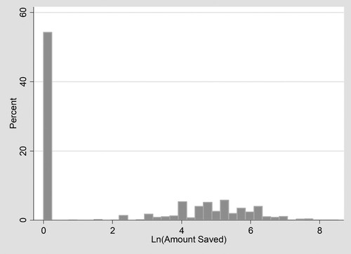
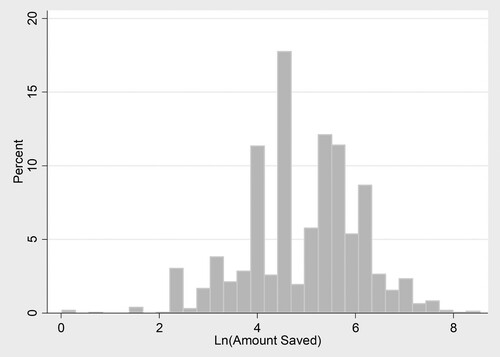
Figure 2. Distribution of the amount saved where saving is greater than zero.

As well as exploring monthly saving, which can be regarded as a flow into savings accounts, we also explore the effects of health status on the stock of financial assets held. It is important to distinguish between the stock and the flow of savings, given that the stock of financial assets arguably reflects long term saving behaviours, whilst the flow into savings in the previous month captures short term saving decisions. Consequently, health may have distinct impacts on both these outcomes. Such analysis relating to the stock of financial assets ties in with existing studies on health and wealth; for example, Adams et al. (2003) and Hurd and Kapteyn (2003) amongst other studies, generally find a positive association between better health and household wealth. Our measure of the stock of financial assets is defined from the question:

I'd like to ask about any savings or investments you may have. Which of these savings accounts do you have, if any? Savings or deposit accounts, National Savings Accounts, ISA – cash only, ISA – stocks and shares, or PEPs, Premium Bonds or Other types of savings accounts.

Individuals are then asked the monetary amount held in each of these assets. The sum of these responses forms the dependent variable relating to the stock of financial assets held. In line with the saving variable, the natural logarithm of financial assets is taken to account for the skewed nature of the variable and, for those individuals reporting that they hold no financial assets, this variable takes the value of zero. The distributions relating to financial assets, both including and excluding zero financial asset holding, are presented in Figures 3 and 4, respectively, with summary statistics presented in Table 1.

Figure 3. Distribution of financial assets.

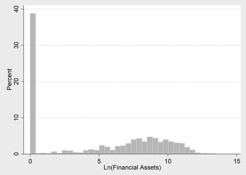
Figure 4. Distribution of financial assets where financial assets are greater than zero.

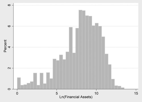
Table 1. Summary Statistics: Dependent Variables

Variable	Mean	(Std. Dev.)
Save (Binary)	45.85%
Ln(Amount Saved) (All Individuals)	2.269	(2.591)
Amount Saved (All Individuals)	119.605	(275.314)
Ln(Amount Saved) (Individuals who save)	4.948	(1.173)
Amount saved (Individuals who save)	260.84	(358.465)
Financial Investments (Binary)	61.90%
Ln(Financial Investments) (All individuals)	4.911	(4.349)
Financial Assets	11,798.75	(37,490.32)
Ln(Financial Investments) (Individuals who hold financial assets)	7.934	(2.562)
Financial Assets (Individuals who hold financial assets)	19,060.40	(46,179.05)
Unsecured Debt (Binary)	39.2%
Ln(Unsecured Debt) (All individuals)	3.109	(4.003)
Unsecured debt (All individuals)	2,770.385	(7,360.036)
Ln(Unsecured Debt) (Individuals who hold unsecured debt)	7.926	(1.630)
Unsecured debt (Individuals who hold unsecured debt)	7062.382	(10383.72)
N	3,365

Notes: Saving is based on the questions: “Do you save any amount of your income, for example, by putting something away now and then in a bank, building society, or Post Office account other than to meet regular bills? About how much, on average, do you manage to save a month?” Financial investments are based on the questions: “I'd like to ask about any savings or investments you may have. Which of these savings accounts do you have, if any? Savings or deposit accounts, National Savings Accounts, ISA - cash only, ISA - stocks and shares, or PEPs, Premium Bonds or Other types of savings accounts”; and “What is the amount held in each of these accounts”. Debt holding is based on the question: “I would now like to ask you about any other financial commitments you may have apart from mortgages. For which, if any, of these items do you currently owe any money? Please do not include credit card and other bills being fully paid off in the current month”; and “About how much in total is owed?” If an individual responds “yes” to the first question, the binary variable is equal to one, zero otherwise. The amount of the variable is then captured by the second question.

Finally, the stock of financial assets held may be related to the stock of debt held. Indeed, a small number of studies have explored the relationship between debt and health. For example, Drentea and Lavrakas (2000) report that both credit card debt and stress regarding debt are inversely associated with good health, and Brown, Taylor, and Wheatley Price (2005) find that unsecured debt is inversely related to psychological well-being. In addition, Keese and Schmitz (2014) report that a variety of debt measures are strongly correlated with satisfaction with health and mental health once unobserved individual heterogeneity is accounted for. Hence, we explore the robustness of our results relating to the effect of health on the stock of financial assets held by jointly modelling the stock of financial assets and the stock of debt held. The level of unsecured debt is generated from the responses to the following questions:

I would now like to ask you about any other financial commitments you may have apart from mortgages. For which, if any, of these items do you currently owe any money? Please do not include credit card and other bills being fully paid off in the current month

and “About how much in total is owed?” From the responses to these questions, in line with the other financial variables, we construct a variable which captures the natural logarithm of the level of unsecured debt. For those individuals reporting that they hold no unsecured debt, the variable takes the value of zero.

3.2. Health measures

As stated in Section 1, an important contribution of our paper lies in our comprehensive analysis of the implications of how health is measured for the estimated relationship between saving and health, which has attracted limited attention in the existing saving literature. We explore the effects of three different measures of health, namely, SAH, the SF-12 index and, finally, a set of biomarkers.⁷

Overall SAH is measured on a five-point scale classified from the question, ‘In general, would you say your health is excellent/very good/good/ fair/poor’; this variable is coded so that a higher score represents better health. This health measure has been extensively used in previous studies in this area and is arguably a reasonable proxy for health risk since it may contain private information on health and health related behaviours that are predictive of future health and are known only to the respondent. However, SAH measures are subject to well-known recall and reporting biases (Bound 1991), and, as a result, they conflate health information with other potentially unobservable information on respondent characteristics, such as labour market preferences and personality traits, which may also influence savings behaviour. Secondly, the SF-12 index is derived from responses to the twelve questions that make up the SF-12 measure of health related quality of life. The index is preference rated using results from a UK population sample to weight the different dimensions of health, such as pain and physical functioning (Brazier and Roberts 2004). The result is a continuous index, where one represents full-health and zero is equivalent to being dead.⁸

Finally, we explore a range of biomarkers collected during the nurse visit. Biomarkers have not been used in previous studies on saving and may provide important insights into the relationship between objective measures of health and financial behaviour. Table A1 in the appendix provides more detail on the biomarkers used and Table 2 presents the associated summary statistics. In the subsequent analysis, where we explore specific biomarkers, following standard practice, see, for example, Chandola and Zhang (2018) and Koda et al. (2016), a natural logarithm transformation of the biomarker measures is used to account for skewed distributions and to allow the results to be interpreted as the effect of a percentage change in the biomarker measure on the dependent variable.

Table 2. Summary statistics: health measures.

Health measure	Mean	Standard deviation
Composite Biomarkers
Allostatic Load – Clinical Cut	3.117	(2.019)
Allostatic Load – Z-Score	−0.343	(6.907)
Individual Biomarkers
General Health
Ln(CHL/HDL)	1.282	(0.344)
CHL/HDL	3.832	(1.433)
Ln(HbA1c)	3.557	(0.154)
HbA1c	35.538	(7.065)
Ln(BMI)	3.311	(0.185)
BMI	27.919	(5.786)
Inflammatory Markers
Ln(CRP)	0.236	(0.941)
CRP	1.950	(1.927)
Liver Function
Ln(ALB)	3.856	(0.057)
ALB	47.376	(2.678)
Self-Assessed Health Measures
SF-12	0.788	(0.134)
SAH	2.564	(1.062)
N	3,365

Notes: Ln(.) denotes natural logarithm. Allostatic load – clinical cut is defined as the sum of the binary variables indicating whether individuals have non-normal levels based on clinical guidance of cut-off points whilst the Z-score measure of allostatic load is a continuous explanatory variable, where an individual's Z-score represents the absolute value of the standardised distance between their level of a given biomarker and the population mean for that biomarker and summed across all biomarkers. CHL/HDL is the ratio of total cholesterol to high density cholesterol. HbA1c is a measure of glycated haemoglobin; an indicator of diabetes risk and is measured in mmol/mol. CRP, c-reactive protein is an inflammatory marker measured in mg/L. Alb is indicative for Albumin, and is measured in g/L. BMI is defined as kg/m². SF-12 is the preference based continuous index derived from the Short Form 12 questionnaire, whilst self-assessed health (SAH) is based on the question: ‘Overall how is your health?’, measured on a five-point scale ranging from ‘excellent’ to ‘very poor’.

We consider a range of biomarkers for general health. One set of biomarkers is particularly associated with being overweight or obese and the subsequent health problems this causes; these are namely the ratio of total cholesterol to high density cholesterol (CHL/HDL), the level of glycated haemoglobin (HbA1c), and the anthropometric measure, body mass index (BMI). These markers are risk factors for a number of chronic conditions including cardiovascular disease (CVD), cancer, diabetes, disability at older age and decreased life expectancy (Musaad and Haynes 2007).⁹ Secondly, we consider a biomarker which captures inflammation and infection, namely C-reactive protein (CRP). This measure is elevated due to the presence of chronic conditions such as diabetes, rheumatoid arthritis and heart disease, and it has been shown to be predictive of CVD and mortality (Danesh et al. 1998; Sesso et al. 2003).¹⁰ Elevated CRP can also be the body's reaction to stress (Fuligni et al. 2009). Finally, we consider a measure of liver function; namely, albumin (ALB). As well as being a general health measure, poor liver function is also associated with alcohol and drug use, in addition to obesity (van Beek et al. 2014).

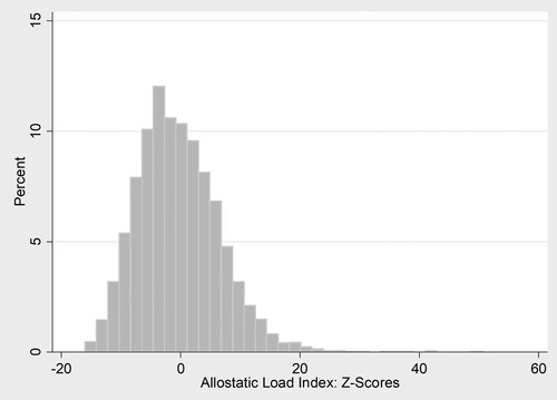
As well as these individual biomarkers, we also explore two commonly used composite measures. Firstly, allostatic load represents the cumulative impact of stressors on the body (Seeman et al. 1997); it is associated with increased risk for mortality, CVD, and declines in cognitive and physical function (Seeman et al. 2002). A health risk index is based on non-normal levels of the biomarkers (Levine and Crimmins 2014). It is the sum of the binary variables indicating whether individuals have non-normal levels for each biomarker based on clinical guidance of cut-off points.¹¹ Higher values of the index are indicative of worse health, see Figure 5 for the distribution of this measure. Secondly, a Z-score measure of allostatic load is entered in our model as a continuous explanatory variable, where an individual's Z-score represents the absolute value of the standardised distance between their level of a given biomarker and the population mean for that biomarker, see Figure 6. A score of 1 denotes whether the individual is either one standard deviation above or below the mean, and the scores are summed (Seplaki et al. 2005). The Z-score measure differs from the simple allostatic load because it provides a continuous rather than categorical measure of physiological function and thus preserves more of the information from the individual biomarkers; the results from Seplaki et al. (2005) suggest that it may be a better predictor of a wider array of health outcomes.

Figure 5. Allostatic load index: clinical cut-offs.

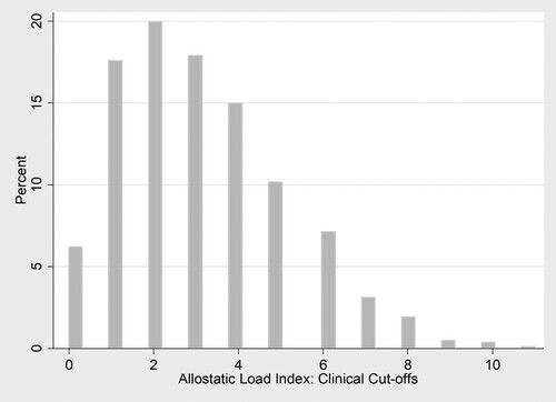
Figure 6. Allostatic load ndex: z-scores.

Given that there may be unobserved characteristics that influence both financial and health decisions, we instrument all of the biomarker outcomes using a measure of physical activity.¹² This is based on responses to the question: ‘On a scale of 0 to 10, with 0 being “doing no sport at all” to 10 being “very active through sport”, where would you rank yourself?’ Conceptually, this measure is a self-reported rating of how active an individual perceives themselves to be, and it is strongly predictive of health outcomes. This measure should not be directly related to financial behaviours, except through an individual's health status. In addition, this variable was collected in wave 2, and so predates the health and financial outcomes, which helps to mitigate potential reverse causality. We acknowledge that there could be unobservable characteristics, which affect all three outcomes (for example, behavioural reasons such as present bias) and so we could still potentially encounter the problem of endogeneity.¹³ Predicted values of the health measures are then included in the models of saving behaviour.

To summarise, we are able to capture a variety of measures of health ranging from completely subjective (SAH) through to completely objective (biomarkers). Another important distinction between these different measures is the extent to which they are known and understood by the respondents. This is important because it helps us to understand the type of information contained in these measures and how they might affect financial behaviour. SAH and the SF-12 index are subjective reports, reflecting the individual's own assessment of their health; so by definition these are known and understood by the individual.

The biomarkers are likely to be the least familiar to the individuals, and we stress here that our study does not require the respondent to know the results of their biomarker tests or to understand the implications of the results. These markers are the same as those commonly used in standard tests carried out for diagnostic purposes or in a general medical examination. As a result, some respondents will have been made aware of their test results in a health care setting. In such a setting, it is likely that the individual is not familiar with the biomarkers themselves, but instead has been informed about the health implications. For example, rather than explaining an elevated HBA1c level, the health care professional is more likely to inform the patient that they have signs of diabetes or pre-diabetes. Further, the biomarkers can capture sub-clinical conditions, which are not known to the individual. It is also possible that for some of our respondents the blood tests undertaken as part of the UKHLS nurse visit will be the only time they have had their biomarkers measured. If this is the case, they will have no knowledge of their results because these were not communicated to respondents as part of the anonymised survey protocol.¹⁴ The biomarker measures of health could therefore capture underlying investments in health which could then be associated with saving decisions. As a result, knowing or understanding the health measures is not necessary for our analysis, if these health measures are capturing broader behavioural factors.

3.3. Model specification

In the two-part model, we allow a number of characteristics to influence the decision to save and the amount saved as follows. In both parts of the model, in addition to the measures of health detailed in Section 3.2 above, based on the existing literature outlined in Section 1, see for example, Browning and Lusardi (1996), Guariglia (2001), Guariglia and Rossi (2004), Rossi (2009), Fisher and Montalto (2010) and Brown et al. (2017), we control for: gender; age and age squared; marital status, captured by variables indicating married, divorced, or widowed, with single being the omitted category; highest level of education captured by variables indicating degree, other high level qualification, A-level, GCSE, or other qualification, while below GCSE level is the omitted category; race, as measured by a white binary variable; the number of children in the household; employment status indicating employed, self-employed or retired with not currently working being the omitted category; and the natural logarithm of monthly household income. We also include 11 regions of residence controls. Hence, for purposes of comparison, our set of explanatory variables is standard in that it follows the existing literature.

We include two additional controls in the binary part of the model. The first additional control is a binary indicator for being in arrears in the last 12 months in at least one of: council tax, household bills (such as electricity, gas, water rates, telephone) or housing payments (that is, rent or mortgage). The second additional control is an eight-point index of material deprivation, which is based on responses indicating the number of areas which people state that they have difficulty finding money for. These areas are namely: holidays; entertaining friends and family; shoes; keeping the house in a decent state of repair; contents insurance; furniture; and major electrical goods (such as a washing machine). We would expect such measures of financial hardship to be related to saving behaviour at the extensive margin, that is, the ability to save with financial hardship acting as a barrier to saving (see, for example, Brown, Ghosh, and Taylor 2014). Table 3 presents summary statistics for the explanatory variables used in the empirical analysis.

Table 3. Summary statistics: independent variables.

Variables	Mean	Standard Deviation
Age	44.74	(10.48)
Age Squared	2111.78	(911.54)
Female*	56.7
Education (Omitted Category: Below GCSE)
Degree*	29.5
Other Higher Qualification*	14.6
A-Level*	21.1
GCSE*	21.4
Other Qualification*	7.49
Relationship Status (Omitted Category: Single/never married)
Married*	72.60
Divorced*	11.4
Widow*	1.43
Number of Children	0.73	(0.99)
Employment status (Omitted Category: Unemployed/Not in the labour force)
Employed*	70.60
Self-Employed*	9.72
Retired*	3.15
Ln(Household Monthly Income)	8.18	(0.67)
Household Monthly Income	4364.10	(2831.39)
Region (Omitted Category: Residing in London)
North East*	6.45
North West*	11.53
Yorkshire*	9.21
East Midlands*	10.37
West Midlands*	9.26
East*	10.22
South East*	15.96
South West*	11.68
Wales*	2.64
Scotland*	4.93
Arrears*	13.88
Material Deprivation	1.420	(2.02)
N	3,365

Note: Mean and standard deviation are reported for continuous variables and proportions are reported for binary independent variables. *denote binary variables.

4. Results

We initially discuss the results for our two-part model of saving behaviour. We briefly consider the effects of a range of standard socioeconomic and demographic variables and then focus on the effect of health status on saving behaviour. Specifically, Table 4 presents the results from our baseline specification, which contains no health measures for comparison with the existing literature on saving, whereas in Table 5, the health measures are included. We then explore the influence of health status on the stock of financial assets held (Table 6), and, finally, we estimate a joint model of financial asset and debt holding based on the copula approach detailed above (Table 7). Throughout Tables 5–7, the health measures are included individually, in conjunction with the independent variables in the baseline specification.

Table 4. A semi-continuous model of monthly saving.

	Binary Part			Continuous Part
Independent Variables	Mean	2.50%	97.50%	Mean	2.50%	97.50%	Marginal Effects†
Age	−0.528	−1.206	0.148	−0.004	−0.048	0.039	−0.461
Age Squared	0.342	−0.350	1.029	0.000	0.000	0.001	0.296
Female	0.060	−0.098	0.219	−0.256*	−0.364	−0.148	−0.205
Degree	0.284	−0.126	0.704	0.612*	0.290	0.938	0.832
Other Higher Qualification	0.296	−0.126	0.730	0.450*	0.117	0.791	0.678
A-Level	0.243	−0.163	0.671	0.368*	0.046	0.703	0.560
GCSE	0.053	−0.358	0.481	0.105	−0.226	0.440	0.150
Other Qualification	0.065	−0.419	0.543	0.013	−0.362	0.392	0.068
Married	−0.379*	−0.650	−0.105	−0.060	−0.242	0.124	−0.437
Divorced	−0.045	−0.389	0.308	−0.086	−0.335	0.159	−0.126
Widow	0.313	−0.380	1.040	−0.009	−0.488	0.465	0.231
White	0.116	−0.239	0.467	0.063	−0.192	0.319	0.159
Number of Children	−0.073	−0.167	0.019	−0.140*	−0.206	−0.075	−0.203
Employed	0.731*	0.470	1.000	0.438*	0.232	0.647	0.910
Self-Employed	0.345*	0.004	0.688	0.576*	0.313	0.841	0.837
Retired	0.256	−0.250	0.770	0.150	−0.254	0.544	0.351
Ln(Household Monthly Income)	0.234*	0.135	0.335	0.569*	0.465	0.675	0.772
North East	0.062	−0.362	0.490	−0.134	−0.430	0.155	−0.082
North West	0.220	−0.152	0.592	−0.295*	−0.543	−0.043	−0.120
Yorkshire	0.108	−0.277	0.486	−0.029	−0.300	0.243	0.061
East Midlands	0.199	−0.177	0.573	−0.041	−0.296	0.222	0.119
West Midlands	0.166	−0.222	0.545	−0.046	−0.301	0.209	0.089
East	0.175	−0.206	0.546	−0.154	−0.411	0.105	−0.012
South East	0.159	−0.185	0.499	−0.060	−0.297	0.177	0.070
South West	0.130	−0.239	0.502	−0.092	−0.346	0.167	0.015
Wales	−0.263	−0.839	0.301	−0.134	−0.553	0.285	−0.385
Scotland	0.190	−0.257	0.637	−0.282	−0.587	0.028	−0.129
Arrear	−0.069	−0.345	0.201				−0.208
Material Deprivation	−0.493*	−0.553	−0.432				−0.446
N	3,365

Notes: *denotes statistically significant at the 5% level. Mean indicates the estimated coefficient, whilst 2.50% and 97.50% denote the 95% credible interval.

†Marginal effects are calculated in the following way:

Continuous independent variables $\frac{\mathrm{\Delta }E(y|x)}{E(y|x)}=\beta .\frac{\phi ({\mathrm{\Phi }}^{-1}(\pi ))}{\pi }+\gamma$;

Binary independent variables $\frac{\mathrm{\Delta }E(y|x)}{E(y|x)}=\text{ln}\left(\frac{\mathrm{\Phi }(\beta +{\mathrm{\Phi }}^{-1}(\pi ))}{\pi }\right)+\gamma$.

Where $\phi$ and $\mathrm{\Phi }$ are the p.d.f and the c.d.f of the standard normal distribution, respectively, $\beta$ is the coefficient in the binary part of the model, $\gamma$ is the coefficient in the continuous part, whilst π is the probability that saving is positive. In this case we take π to equal the sample proportion, that is, 0.4585.

Table 5. Summary of health measures in the semi-continuous model of monthly saving.

	Binary Part			Continuous Part
Health Measures	Mean	2.50%	97.50%	Mean	2.50%	97.50%	Marginal Effects†
Self-Assessed Health
SAH^¶	0.117*	0.037	0.198	0.149*	0.091	0.208	0.154
SF-12	0.732*	0.098	1.361	0.570*	0.123	1.012	1.204
Biomarkers
Composite Biomarkers
Allostatic Load – Clinical Cut	−0.276*	−0.420	−0.133	−0.100	−0.200	0.001	−0.339
Allostatic Load – Z-Score	−0.528*	−0.798	−0.251	−0.204*	−0.393	−0.014	−0.661
Individual Biomarkers
General Health
Ln(CHL/HDL)	−0.436*	−0.655	−0.212	−0.133	−0.285	0.019	−0.511
Ln(HbA1c)	−0.612*	−0.933	−0.279	−0.249*	−0.479	−0.017	−0.779
Ln(BMI)	−0.278*	−0.432	−0.128	−0.093*	−0.195	0.009	−0.334
Inflammatory markers
Ln(CRP)	−0.204*	−0.324	−0.085	−0.089*	−0.168	−0.007	−0.266
Liver Function
Ln(ALB)	0.743*	0.205	1.273	0.713*	0.346	1.076	1.357
N	3,365

Notes: All health measures are included independently along with the independent variables included in Table 4 and outlined in Section 3.3. The results relating to the control variables are qualitatively the same as those presented in Table 4, that is, they generally display the same sign and significance level.

*denotes statistically significant at the 5% level. Mean indicates the estimated coefficient, whilst 2.50% and 97.50% denote the 95% credible interval.

†Marginal effects are calculated in the following way: Continuous independent variables $\frac{\mathrm{\Delta }E(y|x)}{E(y|x)}=\beta \frac{\phi ({\mathrm{\Phi }}^{-1}(\pi ))}{\pi }+\gamma$; and binary independent variables $\frac{\mathrm{\Delta }E(y|x)}{E(y|x)}=\text{ln}\left(\frac{\mathrm{\Phi }(\beta +{\mathrm{\Phi }}^{-1}(\pi ))}{\pi }\right)+\gamma$. Where $\phi$ and $\mathrm{\Phi }$ are the p.d.f and the c.d.f of the standard normal distribution, respectively, $\beta$ is the coefficient in the binary part of the model, $\gamma$ is the coefficient in the continuous part, whilst π is the probability that saving is positive. In this case, we take π to equal the sample proportion, that is, 0.4585.

^¶ Marginal effect presented is for the change from 0 to 1, corresponding to a change from poor to fair health. The marginal effect is calculated in the following way: $\frac{\mathrm{\Delta }E(y|x)}{E(y|x)}=\frac{1}{(b-a)}\text{ln}\left(\frac{\mathrm{\Phi }(\beta b+{\mathrm{\Phi }}^{-1}(\pi ))}{\mathrm{\Phi }(\beta a+{\mathrm{\Phi }}^{-1}(\pi ))}\right)+\gamma$. The marginal effects relating to changes from fair to good health, good to very good health, and very good to excellent health are 0.141, 0.127 and 0.113, respectively.

Table 6. Summary of health measures in semi-continuous model of financial assets.

	Binary Part			Continuous Part
Health Measures	Mean	2.50%	97.50%	Mean	2.50%	97.50%	Marginal effects^†
Self-Assessed Health
SAH^¶	0.139*	0.057	0.222	0.359*	0.255	0.465	0.307
SF-12	0.238	−0.397	0.860	1.725*	0.902	2.539	1.872
Biomarkers
Composite Biomarkers
Allostatic Load – Clinical Cut	−0.235*	−0.385	−0.083	−0.366*	−0.555	−0.175	−0.511
Allostatic Load – Z-Score	−0.432*	−0.724	−0.144	−0.735*	−1.093	−0.377	−1.001
Individual Biomarkers
General Health
Ln(CHL/HDL)	−0.352*	−0.588	−0.114	−0.537*	−0.829	−0.250	−0.754
Ln(HbA1c)	−0.551*	−0.891	−0.210	−0.919*	−1.349	−0.486	−1.258
Ln(BMI)	−0.228*	−0.387	−0.068	−0.382*	−0.579	−0.187	−0.522
Inflammatory markers
Ln(CRP)	−0.179*	−0.302	−0.054	−0.300*	−0.450	−0.146	−0.410
Liver Function
Ln(ALB)	0.837*	0.305	1.380	1.948*	−2.439	−0.052	−0.734
N	3,365

Notes: All health measures are included independently along with the independent variables included in Table 4 and outlined in Section 3.3. The results relating to the control variables are qualitatively the same as those presented in Table 4, that is, they generally display the same sign and significance level.

*denotes statistically significant at the 5% level. Mean indicates the estimated coefficient, whilst 2.50% and 97.50% denote the 95% credible interval.

† Marginal effects are calculated in the following way: Continuous independent variables $\frac{\mathrm{\Delta }E(y|x)}{E(y|x)}=\beta \frac{\phi ({\mathrm{\Phi }}^{-1}(\pi ))}{\pi }+\gamma$; and binary independent variables $\frac{\mathrm{\Delta }E(y|x)}{E(y|x)}=\text{ln}\left(\frac{\mathrm{\Phi }(\beta +{\mathrm{\Phi }}^{-1}(\pi ))}{\pi }\right)+\gamma$. Where $\phi$ and $\mathrm{\Phi }$ are the p.d.f and the c.d.f of the standard normal distribution, respectively, $\beta$ is the coefficient in the binary part of the model, $\gamma$ is the coefficient in the continuous part, whilst π is the probability that saving is positive. In this case, we take π to equal the sample proportion, that is, 0.6190.

^¶ Marginal effect presented is for the change from 0 to 1, corresponding to a change from poor to fair health. The marginal effect is calculated in the following way: $\frac{\mathrm{\Delta }E(y|x)}{E(y|x)}=\frac{1}{(b-a)}\text{ln}\left(\frac{\mathrm{\Phi }(\beta b+{\mathrm{\Phi }}^{-1}(\pi ))}{\mathrm{\Phi }(\beta a+{\mathrm{\Phi }}^{-1}(\pi ))}\right)+\gamma$. The marginal effects relating to changes from fair to good health, good to very good health, and very good to excellent health are 0.288, 0.269 and 0.249, respectively.

Table 7. Joint semi-continuous model of financial assets and unsecured debt holding.

	Financial Assets						Total Unsecured Debt
	Binary Part			Continuous Part			Binary Part			Continuous Part
Health Measures	Mean	2.5%	97.5%	Mean	2.5%	97.5%	Mean	2.5%	97.5%	Mean	2.5%	97.5%
Composite Biomarkers
Allostatic Load – Clinical Cut	−0.144*	−0.233	−0.052	−0.375*	−0.558	−0.181	0.018	−0.065	0.105	−0.030	−0.190	0.134
Allostatic Load – Z-Score	−0.258*	−0.423	−0.086	−0.771*	−1.122	−0.407	0.067	−0.090	0.222	−0.002	−0.294	0.311
Individual Biomarkers
General Health
Ln(CHL/HDL)	−0.218*	−0.361	−0.091	−0.593*	−0.875	−0.31	0.029	−0.101	0.153	0.038	−0.211	0.270
Ln(HbA1c)	−0.238*	−0.376	−0.106	−0.796*	−1.111	−0.498	−0.009	−0.132	0.115	0.183	−0.059	0.439
Ln(BMI)	−0.120*	−0.215	−0.024	−0.357*	−0.561	−0.153	0.064	−0.022	0.151	−0.014	−0.184	0.153
Inflammatory markers
Ln(CRP)	−0.110*	−0.180	−0.037	−0.321*	−0.476	−0.164	0.028	−0.044	0.096	−0.001	−0.130	0.128
Liver Function
Ln(ALB)	0.259*	0.097	0.421	1.076*	0.714	1.433	0.012	−0.148	0.162	−0.245	−0.568	0.042
Self-Assessed Health
SAH	0.089*	0.035	0.139	0.387*	0.278	0.499	−0.050	−0.101	0.001	0.095*	0.003	0.183
SF-12	0.018	−0.031	0.068	0.242*	0.136	0.359	−0.052*	−0.100	−0.007	0.077	−0.012	0.164
N	3,365

Notes: All health measures are included independently along with the independent variables included in Table 4 and outlined in Section 3.3. The results relating to the control variables are qualitatively the same as those presented in Table 4, that is, they generally display the same sign and significance level.

*denotes statistically significant at the 5% level. Mean indicates the estimated coefficient, whilst 2.50% and 97.50% denote the 95% credible interval.

4.1. The two-part Bayesian model of monthly saving

The estimated coefficients and corresponding unconditional marginal effects relating to the demographic variables and health measures from estimating the two-part model of saving are presented in Tables 4 and 4, respectively.¹⁵ When the health measures are included, the estimated coefficients for the other control variables remain very similar to those reported in Table 4 so for the purposes of brevity we do not repeat them in Table 5.

Looking first at Table 4, generally, in line with the existing literature, see for example Fisher and Montalto (2010), Brown and Taylor (2008), Guariglia and Rossi (2004), Rossi (2009), education, gender, family composition, employment status and household income all have statistically significant associations with saving behaviour. The results suggest that many variables have distinct associations with the propensity to save and the level of savings, demonstrating the advantage of our two-part modelling approach over the empirical strategies commonly employed in the existing literature. For example, education has a statistically significant positive association with the amount saved, but not on the decision to save.¹⁶ This effect is above and beyond the effect of income and suggests that the decision to save in the short term is dictated by the level of financial resource, captured by income, as opposed to an individual's level of education. In contrast, in addition to influencing the amount of saving, the level of income serves to determine whether or not saving occurs, with low income, for example, potentially acting as a barrier to saving behaviour. Compared to having below GCSE level education, conditional on saving, holding a degree is associated, on average, with a 61.2% higher saving amount. Furthermore, conditional on saving, females save a lower amount than their male counterparts as do individuals with dependent children, see for example, Brown and Taylor (2008). In line with the existing literature (see, Fisher and Montalto 2010; Brown et al. 2017), income and employment status display positive associations with both the decision to save and the amount saved. For example, income is positively associated with saving, that is, the unconditional marginal effect reveals that a 1% increase in income is associated with a 0.77% higher level of saving. Further, the two-part model reveals the relative magnitudes of this association in the binary and continuous parts of the model; a 1% increase in household monthly income is associated with a 0.23% higher (odds Ratio (OR) = ${1.01}^{0.234}=1.0023$) probability of saving and, conditional on saving, is associated with a 0.57% increase in the amount saved. Moreover, relative to being out of the labour force, being employed is associated with double the probability of saving, and is associated with a 43.8% increase in the level of saving, a result similar in magnitude to Fisher and Montalto (2010).¹⁷

Table 5, the focus of our study, presents the relationship between our different health measures and saving. Once again, the results demonstrate the importance of accounting for two distinct data generating processes, given that several health measures have different impacts, in terms of both magnitudes and statistical significance, on the decision to save and the amount saved. The results indicate that SAH and the SF-12 index have significant relationships with saving behaviour, over and above the wide range of demographic and socioeconomic controls specified in Table 4. In accordance with the theory discussed in Section 1, better health is associated with both an increased likelihood of saving and higher levels of the amount saved. Considering the relationship between SAH and saving behaviour reveals that moving from poor to fair health (the lowest two categories) has a greater association with saving behaviour than a change from very good to excellent health (the highest two categories). Specifically, the unconditional marginal effects indicate that the change from poor to fair health is associated with a 15.4% higher level of saving, whilst a change from very good to excellent health is associated with an 11.3% higher level of saving. Turning to the less subjective SF-12 index measure of health, the unconditional marginal effect indicates that a 10 percentage point (pp) increase in the SF-12 index is associated with 12% higher saving. Separating this effect into effects on the propensity to save and the amount saved reveals that it is associated with an increase in the probability of saving by 20.8% (OR = $\text{exp}$(0.732)), and, conditional on saving, it is associated with a 5.70% increase in the amount saved. Hence, both SAH and the SF-12 index exhibit a positive association in both parts of the model. These results support a positive relationship between being in better health and saving. These effects exist over and above the effects of income, and potentially point to health capturing unobserved behavioural or lifestyle factors, which influence both health and saving behaviours, such as time preferences and risk aversion.

Turning to the effects of our most objective health measures, the biomarker measures of health, the findings once again highlight the flexibility of our empirical strategy as several biomarkers have distinct impacts in the two parts of the model. For example, a one-point increase in the summary clinical cut-off allostatic load measure is associated with a reduction in the probability of saving by 24.1% ($\text{OR }=\text{exp}(-0.276))$, however, it is not significantly associated with the amount saved. In contrast, the Z-score measure of allostatic load has a negative association with both the decision to save and the amount saved. For the individual biomarkers, the levels of HbA1c, BMI, CRP and albumin all have significant associations in both parts of the saving model, reflecting the fact that worse levels for these markers are associated with both a lower propensity to save and a lower amount saved. For BMI, for example, the magnitudes of these associations reveal that a 1% increase in BMI is associated with a decrease in the probability of saving by 0.3% ($\text{OR}={1.01}^{-0.278}$), and conditional on saving, is associated with a fall in the amount saved by 0.15%. The cholesterol measure (CHL-to-HDL ratio) has a positive association with the probability of saving but not the amount saved. Given that these measures are generally unobserved to the individuals, we argue that there are unobservable behavioural traits, such as time preference, that are associated with a lower level of investment in health and saving.

Overall, the results indicate that health has a significant association with saving behaviours over and above an extensive range of demographic controls, and this association varies according to how health is measured. The results suggest that the largest effects are found when health is measured using SAH, followed by the SF-12 index and then by the composite biomarker measures. With respect to the potential mechanisms underlying the relationship between health and saving behaviour, this is consistent with the argument that the subjective health measures conflate biomedical health information with other (unobserved) information on respondent characteristics such as lifestyle factors related to, for example, diet and exercise and/or individual health perception as well as attitudes related to anticipated life expectancy and the associated financial planning. The relative size of the effects suggests that this additional information has an important influence on saving behaviour, in addition to the objective biomedical information contained in the biomarkers.

Furthermore, it is important to acknowledge that in order to capture the indirect effects of health on saving operating via productivity and income, we have controlled for income in our specification. Hence, the direct effect of health on saving behaviour may be capturing effects related to costs associated with health care and/or costs associated with healthy versus unhealthy lifestyle considerations. The fact that our health measures influence saving behaviour above and beyond the influence of income suggests that these mechanisms are potentially important, thereby highlighting the significance of our findings.

In contrast to the subjective measures of health, the objective biomarker measures are likely to be the least familiar to the individuals. However, the biomarkers are still significantly associated with savings and while we cannot claim causal effects, we suggest that one possible causal pathway is that the biomarkers are reflecting unobserved behavioural characteristics, which affect both health and savings behaviours. Our analysis has shed light on the relationship between health and household financial decisions, however, it does not claim causality. This is an area, given the data available, which we are unable to test empirically. However, we suggest that unobservable behavioural factors, in particular time preference and risk preference underlie the potential causal pathways between health and financial decisions. Those individuals who have less present bias and are more risk averse are more likely to invest in their health (Grossman 1972), which will be reflected in ‘good’ biomarker test results; they are also more likely to save for the future.

4.2. The two-part Bayesian model of the stock of financial assets

Table 6 is similar to Table 4, but this time focuses on modelling the relationship between health and financial asset holding, that is, a stock rather than flow measure of saving behaviour. It is interesting to explore the stock of financial assets, in addition to the flow of monthly saving, given that the level of financial assets arguably captures long term, opposed to short term, saving decisions and, as a consequence, health could have a differential impact on this outcome. The results suggest that health plays an important role here as well and once again different health measures have distinct impacts on the decision to hold financial assets and on the amount held. Specifically, better SAH is associated with a higher propensity to hold financial assets and, on average, increases in the amount of assets held. In line with the results relating to saving, there is a larger association at the bottom of the SAH distribution compared to at the top. The SF-12 index only displays a positive relationship with the amount of financial assets held. Conditional on holding financial assets, a 10pp increase in the SF-12 index is associated with a 17.3% increase in the level of assets. This is significantly larger than the association with monthly saving, suggesting that health status has implications for saving decisions in both the short run and the long run.

The biomarker results show that better health is positively associated with the level of financial assets. For example, the measures of allostatic load are inversely related to both the propensity to hold financial assets and, conditional on holding financial assets, the amount of assets. Furthermore, similar effects are present for all of the individual biomarkers. For example, the unconditional marginal effects indicate that 1% increases in BMI and CRP levels are associated with reductions in the amount of financial assets by 0.52% and 0.41%, respectively. Moreover, the two-part model reveals that, conditional on holding financial assets, 1% increases in BMI and CRP are associated with falls in the level of financial assets by 0.38% and 0.30%, respectively. Moreover, a 1% lower level of CHL-to-HDL ratio is associated with a 0.35% ($\text{OR}={1.01}^{-0.352})$ lower propensity to hold financial assets and, conditional on holding financial assets, a fall in the level of financial assets by 0.54%. Overall, our findings related to financial asset holding generally accord with those for monthly saving, with many health measures having distinct associations in each part of the model. The results also suggest that the associations between health and financial assets are greater than those found for monthly savings. This indicates that the effects of health have implications for both short term and long term saving decisions.

Once again, the finding that all of our health measures (SAH, SF-12 and biomarkers) are important, given the difference in individuals’ awareness of these health measures, points to the relevance of unobservable characteristics, such as time preference, which are associated with both financial asset accumulation and investment in health. In addition, as in the case of our findings for the flow of savings, our results arguably provide limited evidence supporting precautionary saving motives, see, for example, Lusardi (1998). Specifically, the precautionary saving motive suggests that households accumulate wealth to self-insure against unexpected outcomes (such as future loss of income or higher medical expenditures). If current health is a predictor of future health uncertainty, precautionary saving arguments would predict that those in worse health would save more in order to self-insure against adverse future outcomes. In contrast, our results suggest that savings are positively associated with better health. Furthermore, the biomarker measures of health support this positive association and, as argued above, these specific health measures may be unknown to the individual. Such findings suggest that other mechanisms are at play here such as the lost productivity (resulting in lower earnings) associated with poor health preventing both the flow into and the accumulation of savings and financial assets. More generally, such findings can also be attributed to the fact that the UK National Health Service is free at the point of use, so that the need to accumulate assets to act as a buffer against future health expenditures is not as pronounced as it is, for example, in the US, which does not have a comparable universal healthcare system.

4.3. The copula approach for jointly modelling financial assets and debt

As stated above, the relationship between the stock of financial assets and health may be influenced by debt holding. Hence, Table 7 presents the results from exploring the robustness of our findings for asset holding when estimating a joint model of financial asset and debt holding. This is based on the copula approach described in Section 2.3. For brevity, we only present the results relating to SAH and the SF-12 index in addition to the biomarker health outcomes.

For the more subjective health measures, in line with the previous results, the results relating to SAH reveal that better health is associated with an increased likelihood of holding financial assets and holding a higher amount of these assets. The SF-12 index is also significantly associated with financial asset holding, in line with the results discussed above. Turning our attention to the objective measures of health, in line with the previous results, allostatic load is inversely related to the amount of financial assets held. Considering the individual biomarkers, the results from the joint modelling approach accord with the results from the two-part model discussed above. Specifically, CRP, BMI, CHL to HDL ratio, HbA1c and Albumin are all significantly associated with financial asset holding, and generally display a significant association with both the decision to hold financial assets and the amount of assets held.

In contrast, the results indicate that health has a limited association with debt accumulation in our sample. For SAH, the coefficient on the decision to hold debt is negative, although statistically insignificant, whilst it is positively associated with the level debt held. In contrast, the SF-12, has a statistically significant negative association with the propensity to hold debt, whilst this has a statistically insignificant impact on the level of debt held. The results relating to debt suggest there is little evidence of an association between the objective measures of health and debt levels. The finding that self-assessed health measures, as opposed to the biomarker measures of health, influence debt decisions suggests that debt decisions are driven by an individual's perceptions about their health status. Again, it is important to stress that the UK has a free at the point of use health care system and, as such, we would not anticipate that individuals need to borrow in order to access health care, in contrast to, for example, the US. The findings suggest that there are unobserved factors which influence subjective health and debt accumulation, but not objective biomarker measures of health. Importantly, this finding highlights that debt behaviours are not influenced by the same mechanisms and unobservable characteristics as saving behaviours.

5. Conclusion

We have developed a flexible Bayesian two-part framework to analyse the effects of health on financial behaviours, namely saving and financial asset holding, in Britain. This framework is applicable where there is a prior belief that there are separate decision-making processes governing, for example, the decision to save and the amount saved. Analysing data drawn from a UK household panel study, our results confirm that such an approach is highly appropriate with health measures found to have distinct effects across the two decisions. Further, we also contribute to the literature by showing that the effects of health differ depending on how health is measured, an area which has been largely neglected in the existing literature. The vast majority of the existing literature relies on SAH, a purely subjective view of individual health status. In contrast, we have explored a broad range of objective biomarker measures of health, estimating their association with household financial decision-making. The introduction of biomarkers to the saving literature represents an important contribution of our study.

The results confirm that health status is an important determinant of household financial decision-making in Britain. In line with the existing literature, better SAH has a positive influence on saving behaviour, and our results indicate that it has a significant association with both the decision to save and the amount saved. In addition, we find that more objective health measures also influence saving. We consistently find that composite biomarker measures of health status, as measured by allostatic load, are associated with saving. We also find that individual biomarkers, specifically those relating to general health, and those reflecting chronic conditions such as diabetes risk and overweight status, are associated with saving. Our findings suggest that there are unobservable characteristics, such as time and risk preferences, which simultaneously influence saving decisions and investments in health, as captured by the objective health measures. Future research could seek to explore these causal mechanisms in further detail.

Our findings support an inverse relationship between saving and poor health, which is confirmed by a wide range of health measures, with subjective measures of health revealing a more pronounced association. Furthering our understanding of saving behaviour is important since saving plays a protective role against financial vulnerability in that it provides a buffer for adverse expenditure and income shocks. From a policy perspective, enhancing understanding of the importance of saving through financial education designed to develop financial literacy skills is a potential fruitful way forward. From a health perspective, financial vulnerability may lead to further physical and mental health issues, which in turn may lead to debt accumulation in the context of holdings of low or no savings. Policy interventions related to financial education designed to tackle this cycle may be considered in the context of public health campaigns. Moreover, given that poor health impedes a household's ability to accumulate wealth, policies, which provide support for those in poor health, could help reduce wealth inequalities which are exacerbated by an individual's health status.

Acknowledgements

We are grateful to the Data Archive at the University of Essex for supplying Understanding Society waves 1 to 4 and to Alberto Montagnoli and Gurleen Popli for valuable advice and suggestions. We are also grateful to participants at the Royal Economic Society Conference 2017, Bristol, the European Society for Population Economics Annual Conference 2017, Glasgow, and the Sheffield School of Health and Related Research, Health Economics and Decision Science Seminar Series for helpful comments on earlier versions of the paper. Finally, we are very grateful to the editor and two referees for valuable and constructive comments.

Disclosure statement

No potential conflict of interest was reported by the author(s).

Notes

1 The SF-12 is a multidimensional measure of health comprising 12 questions relating to issues such as pain, physical functioning, social functioning and mental health; a continuous preference based index of health related quality of life was created from the SF-12 by Brazier and Roberts (2004).

2 A double-hurdle model is an alternative econometric specification, which allows independent variables to have different effects on the probability of, for example, saving and on the level of saving if it is non-zero. A potential limitation of this approach is finding suitable instruments to identify the model. Our Bayesian approach does not suffer from this limitation; however, we do include two exclusion restrictions as described below to aid identification. Furthermore, the double-hurdle model has not been extended to the multivariate case, which means that it cannot be used when jointly modelling different aspects of household finances (as in our joint modelling of financial assets and debt discussed in detail below).

3 The General Population Sample excludes both the ethnic minority boost and the BHPS samples. This maintains that the sample is nationally representative and avoids potential panel conditioning relating to BHPS members who have been surveyed for up to 18 waves.

4 We make the assumption that data is missing at random. However, it is plausible that missingness associated with the dependent variables is systematically different across health states. In our setting, we find little evidence that this is problematic; there is a relatively small percentage of missing values associated with the dependent variables and we find limited evidence that there are systematic differences in health across individuals reporting missing and valid responses for the financial variables.

5 We have explored an alternative empirical strategy based on the ratio of monthly saving to household income as opposed to the absolute level of saving. For brevity and in line with the existing literature, we only present results relating to the absolute level of saving, whilst controlling for household income. In addition, we have explored the inclusion of voluntary pension contributions to monthly saving measures. In both cases, we obtain similar results to those presented here.

6 The height of the bars is scaled so that the sum of their heights equals 100. This is implemented in Stata.

7 We have also explored the effect of the number of diagnosed chronic health conditions as a measure of health status. These conditions include, for example, arthritis, emphysema, and diabetes amongst many others. In contrast to the SAH and the SF-12 index, the number of diagnosed health conditions is not significantly associated with the propensity to save, but does have a statistically significant relationship with the amount saved.

8 Theoretically, the SF-12 index can take negative values, which are interpreted as very severe health states considered worse than being dead; however, these are rarely observed in practice.

9 The ratio of CHL-to-HDL is considered as opposed to an individual measure of cholesterol, as in some circumstances this ratio can be a stronger predictor of cardiovascular risk; see Prospective Studies Collaboration (2007) and Davillas and Pudney (2017). Consistent results are found when we include alternative blood fat measures (total cholesterol, HDL, triglycerides).

10 We have also considered fibrinogen, an alternative measure of inflammation, and find similar results to those of CRP.

11 In the construction of the allostatic load measure, we use the full array of biomarkers available in Understanding Society. For those biomarkers with no agreed clinical cut-off, in line with Crimmins et al. (2003), the upper 25% based on the sample distribution is used to define being at risk.

12 We do not instrument the subjective health measures (SF12 and SAH) for two reasons. Firstly, these form the baseline results and are included for the purposes of comparison with the existing literature, see for example, Fisher and Montalto (2010). Secondly, we would argue that it is inappropriate to instrument these subjective health measures with a subjective measure of physical activity, given there may be unobservable characteristics, which influence both subjective measures.

13 In each of the first stage regressions, an F-statistic greater than 10 is achieved, with the instrument also being individually significant. It is important to acknowledge that the selection of instruments is inevitably an area of debate. Unfortunately, there are no formal tests for exclusion restrictions available for use within our Bayesian framework. Our findings are generally robust to entering the biomarkers as exogenous variables. For brevity, these findings are not reported here but they are available on request. We have also explored using alternative instruments, such as smoking and drinking behaviours, which are likely to be associated with the objective measures of health. However, given that these behaviours involve some form of expenditure, they may also directly impact on an individual's ability to save and accumulate financial assets. Consequently, these variables do not satisfy the required exclusion restrictions conceptually. We do find that the general pattern of results is robust to using these different instruments.

14 Before they consent, participants are told that all blood samples are anonymised so when it is tested for research, it will no longer be possible to link it to them, so they will not be told the results. See Understanding Society: The Nurse Visit Information for Participants Leaflet: www.understandingsociety.ac.uk/documentation/health-assessment/fieldwork-documents.

15 Unconditional marginal effects relate to how changes in the independent variables impact on the expected value of the dependent variable, $\frac{\mathrm{\Delta }E(y|x)}{E(y|x)}$. The two-part model also allows the exploration of the conditional marginal effects of the independent variables in the binary and continuous parts of the model. The binary coefficients represent the log odds ratios, whilst, conditional on participation, the coefficients in the continuous part of the model are interpreted in the standard way.

16 It is important to note that education has a statistically significant association with both the decision to hold financial assets and the level of financial assets held. This highlights that education has an important role in long term saving decisions, whereas, short term saving decisions appear to be dictated by financial resources. Full results are available on request.

17 This magnitude is generally in line the existing literature; for example, Fisher and Montalto (2010) report that being unemployed, relative to being employed, reduces the odds of saving by 37% (odds ratio 0.63).

References

- Adams, P., M. D. Hurd, D. McFadden, A. Merrill, and T. Ribeiro. 2003. “Healthy, Wealthy, and Wise? Tests for Direct Causal Paths between Health and Socioeconomic Status.” Journal of Econometrics 112 (1): 3–56.
- Belloni, A., D. Chen, V. Chernozhukov, and C. Hansen. 2012. “Sparse Models and Methods for Optimal Instruments with an Application to Eminent Domain.” Econometrica 80 (6): 2369–2429.
- Benzeval, M., A. Davillas, M. Kumari, and P. Lynn. 2014. Understanding Society: UK Household Longitudinal Study: Biomarker User Guide and Glossary. Colchester: University of Essex.
- Bound, J. 1991. “Self-reported versus Objective Measures of Health in Retirement Models.” Journal of Human Resources 26: 106–138.
- Brazier, J. E., and J. Roberts. 2004. “Estimation of a Preference-based Index Measure of Health for the SF-12.” Medical Care 42 (9): 851–859.
- Brown, S., P. Ghosh, B. Pareek, and K. Taylor. 2017. Financial Hardship and Saving Behaviour: Bayesian Analysis of British Panel Data. IZA, DP No. 10910.
- Brown, S., P. Ghosh, L. Su, and K. Taylor. 2015. “Modelling Household Finances: A Bayesian Approach to a Multivariate Two-part Model.” Journal of Empirical Finance 33: 190–207.
- Brown, S., P. Ghosh, and K. Taylor. 2014. “The Existence and Persistence of Household Financial Hardship.” Journal of Banking and Finance 46: 285–298.
- Brown, S., P. Ghosh, and K. Taylor. 2016. “Household Finances and Social Interaction: Bayesian Analysis of Household Panel Data.” Review of Income and Wealth 62 (3): 467–488.
- Brown, S., and K. Taylor. 2008. “Household Debt and Financial Assets: Evidence from Germany, Great Britain and the USA.” Journal of the Royal Statistical Society: Series A (Statistics in Society) 171 (3): 615–643.
- Brown, S., K. Taylor, and S. Wheatley Price. 2005. “Debt and Distress: Evaluating the Psychological Cost of Credit.” Journal of Economic Psychology 26 (5): 642–663.
- Browning, M., and A. Lusardi. 1996. “Household Saving: Micro Theories and Micro Facts.” Journal of Economic Literature 24: 1797–1855.
- Chandola, T., and N. Zhang. 2018. “Re-employment, Job Quality, Health and Allostatic Load Biomarkers: Prospective Evidence from the UK Household Longitudinal Study.” International Journal of Epidemiology 47 (1): 47–57.
- Crimmins, E. M., M. Johnston, M. Hayward, and T. Seeman. 2003. “Age Differences in Allostatic Load: An Index of Physiological Dysregulation.” Experimental Gerontology 38 (7): 731–734.
- Danesh, J., R. Collins, P. Appleby, and R. Peto. 1998. “Association of Fibrinogen, C-reactive Protein, Albumin, or Leukocyte Count with Coronary Heart Disease: Meta-analyses of Prospective Studies.” Journal of the American Medical Association 279: 1477–1482.
- Davillas, A., and S. Pudney. 2017. “Concordance of Health States in Couples: Analysis of Self-reported, Nurse Administered and Blood-based Biomarker Data in the UK Understanding Society Panel.” Journal of Health Economics 56: 87–102.
- DeVaney, S. A., S. T. Anong, and S. E. Whirl. 2007. “Household Savings Motives.” Journal of Consumer Affairs 41: 174–186.
- Drentea, P., and P. J. Lavrakas. 2000. “Over the Limit: The Association among Health.” Race and Debt. Social Science and Medicine 50 (4): 517–529.
- Feng, X., B. Lu, X. Song, and S. Ma. 2019. “Financial Literacy and Household Finances: A Bayesian Two-part Latent Variable Modelling Approach.” Journal of Empirical Finance 51: 119–137.
- Fisher, P. J., and C. P. Montalto. 2010. “Effect of Saving Motives and Horizon on Saving Behaviors.” Journal of Economic Psychology 31: 92–105.
- Fisher, P. J., and C. P. Montalto. 2011. “Loss Aversion and Saving Behavior: Evidence from the 2007 U.S. Survey of Consumer Finances.” Journal of Family Economic Issues 32: 4–14.
- Frees, E. W., and Y. Sun. 2010. “Household Life Insurance Demand: A Multivariate Two-part Model.” North American Actuarial Journal 14 (3): 338–354.
- Fuligni, A. J., E. H. Telzer, J. Bower, M. R. Irwin, L. Kiang, and S. W. Cole. 2009. “Daily Family Assistance and Inflammation among Adolescents from Latin American and European Backgrounds.” Brain, Behavior, and Immunity 23 (6): 803–809.
- González, L., and B. Özcan. 2013. “The Risk of Divorce and Household Saving Behavior.” Journal of Human Resources 48 (2): 404–434.
- Gropp, R., J. K. Scholz, and M. J. White. 1997. “Personal Bankruptcy and Credit Supply and Demand.” The Quarterly Journal of Economics 112: 217–251.
- Grossman, M. 1972. The Demand for Health: A Theoretical and Empirical Investigation. New York: Columbia University Press.
- Guariglia, A. 2001. “Saving Behaviour and Earnings Uncertainty: Evidence from the British Household Panel Survey.” Journal of Population Economics 14 (4): 619–634.
- Guariglia, A., and M. Rossi. 2004. “Private Medical Insurance and Saving: Evidence from the British Household Panel Survey.” Journal of Health Economics 23 (4): 761–783.
- Hurd, M., and A. Kapteyn. 2003. “Health, Wealth, and the Role of Institutions.” Journal of Human Resources 38 (2): 386–415.
- Keese, M., and H. Schmitz. 2014. “Broke, Ill, and Obese: Is There an Effect of Household Debt on Health?” Review of Income and Wealth 60 (3): 525–541.
- Kennickell, A., and A. Lusardi. 2004. “Disentangling the Importance of the Precautionary Saving Motive.” Working Paper 10888, Cambridge MA, National Bureau of Economic Research.
- Koda, M., I. Kitamura, T. Okura, R. Otsuka, F. Ando, and H. Shimokata. 2016. “The Associations between Smoking Habits and Serum Triglyceride or Hemoglobin A1c Levels Differ According to Visceral Fat Accumulation.” Journal of Epidemiology 26 (4): 208–215.
- Levine, M. E., and E. M. Crimmins. 2014. “A Comparison of Methods for Assessing Mortality Risk.” American Journal of Human Biology 26 (6): 768–776.
- Lusardi, A. 1998. “On the Importance of the Precautionary Saving Motive.” American Economic Review 88 (2): 449–453.
- Lyons, T. J., and A. Basu. 2012. “Biomarkers in Diabetes: Hemoglobin A1c, Vascular and Tissue Markers.” Translational Research: The Journal of Laboratory and Clinical Medicine 159 (4): 303–312.
- Maslow, A. H. 1943. “A Theory of Human Motivation.” Psychological Review 50 (4): 370–396.
- Musaad, S., and E. N. Haynes. 2007. “Biomarkers of Obesity and Subsequent Cardiovascular Events.” Epidemiological Review 29: 98–114.
- Nelsen, R. B. 2006. An Introduction to Copulas. 2nd ed. New York: Springer-Verlag.
- Olsen, M. K., and J. L. Schafer. 2001. “A Two-part Random-Effects Model for Semicontinuous Longitudinal Data.” Journal of the American Statistical Association 96 (454): 730–745.
- ONS (Office of National Statistics). 2020. Quarterly National Accounts: Quarter 1 (Jan to Mar) 2020, Statistical Bulletin.
- Prospective Studies Collaboration. 2007. “Blood Cholesterol and Vascular Mortality by Age, Sex, and Blood Pressure: A Meta-analysis of Individual Data from 61 Prospective Studies with 55 000 Vascular Deaths.” The Lancet 370 (9602): 1829–1839.
- Ricketts, C. F., J. P. Rezek, and R. C. Campbell. 2013. “The Influence of Individual Health Outcomes on Individual Savings Behavior.” The Social Science Journal 50 (4): 471–481.
- Rossi, M. 2009. “Examining the Interaction between Saving and Contributions to Personal Pension Plans: Evidence from the BHPS.” Oxford Bulletin of Economics and Statistics 71 (2): 253–271.
- Seeman, T. E., B. H. Singer, J. W. Rowe, R. I. Horwitz, and B. McEwen. 1997. “Price of Adaptation - Allostatic Load and its Health Consequences.” Archives of Internal Medicine 157: 2259–2268.
- Seeman, T. E., B. H. Singer, C. D. Ryff, G. D. Love, and L. Levy-Storms. 2002. “Social Relationships, Gender, and Allostatic Load across Two Age Cohorts.” Psychosocial Medicine 64: 395–406.
- Seplaki, C. L., N. Goldman, D. Glei, and M. Weinstein. 2005. “A Comparative Analysis of Measurement Approaches for Physiological Dysregulation in an Older Population.” Experimental Gerontology 40: 438–449.
- Sesso, H. D., J. E. Buring, N. Rifai, G. J. Blake, J. M. Gaziano, and P. M. Ridker. 2003. “C-reactive Protein and the Risk of Developing Hypertension.” Journal of the American Medical Association 290: 2945–2951.
- Tooze, J. A., G. K. Grunwald, and R. H. Jones. 2002. “Analysis of Repeated Measures Data with Clumping at Zero.” Statistical Methods in Medical Research 11 (4): 341–355.
- van Beek, J. H., M. H. de Moor, L. M. Geels, M. R. Sinke, E. J. de Geus, G. H. Lubke, C. Kluft, et al. 2014. “The Association of Alcohol Intake with Gamma-Glutamyl Transferase (GGT) Levels: Evidence for Correlated Genetic Effects.” Drug and Alcohol Dependence 134: 99–105.
- Yoshida, A., and A. Guariglia. 2002. “Estimating Saving Functions in the Presence of Excessive-zeros Problems.” The Econometrics Journal 5 (2): 435–456.
- Zou, H., and T. Hastie. 2005. “Regularization and Variable Selection via the Elastic Net.” Journal of the Royal Statistical Society: Series B (Statistical Methodology) 67 (2): 301–320.