Analysing emerging market returns with high-frequency data during the global financial crisis of 2007–2009

Abstract

Nowadays, the majority of stock market trading is performed electronically, based on pre-programmed computer algorithms. We obtain five-minute high-frequency data from the Turkish Stock Exchange to investigate the data-generating process of emerging market returns during the global financial crisis of 2007–2009. We test tail behaviour and how data-generating processes changed during the intraday trading period in both crisis and non-crisis periods. We also examine whether price asymmetry has a significant effect on the diffusion and jump characteristics of emerging market returns. The results identify a clear increase in jumps with infinite activity in crisis periods and a decreased identification of jumps with finite activity in non-crisis periods. In crisis periods, the proportion of large and small jumps increased and the proportion of Brownian motion decreased. We show that data-generating processes are not stable during the intraday trading period, which fluctuates slightly, particularly right after the market opening times in the morning and in the afternoon. Finally, we conclude that there are many more stressful days in crisis periods than in non-crisis periods in emerging markets returns.

KEYWORDS:

• Emerging markets
• high-frequency data
• financial crisis
• Stock market trading

JEL Categories:

• G12

1. Introduction

What is the most appropriate way to model asset prices? Various studies model asset prices with a different base component. For example, in mathematical finance, some studies model stock returns with pure Brownian motion, while others model them with Brownian motion with jumps. In the empirical literature, different types of assets are modelled with Brownian motion and jumps (Dungey and Gajurel 2014; Dungey, Holloway, and Yalaman 2012; Erdemlioglu, Laurent, and Neely 2013; Aït-Sahalia and Jacod 2012; Todorov and Tauchen 2010). Therefore, it is reasonable to assume that asset prices are best described jointly with Brownian motion with jumps.

A number of studies employ high-frequency data to examine different emerging market issues during periods of normal economic conditions. For example, Sensoy (2016) uses tick-by-tick data from 4 January 2010 to 31 December 2013 and reports that among several developed countries, only US monetary policy and macroeconomic announcements raise commonality in liquidity in the Turkish stock market. Sensoy (2017) also documents that institutional ownership leads to an increase in commonality in liquidity for mid-to-large cap firms in the sample containing order book data from BIST with all orders coming to the stock exchange from 4 January 2010 to 31 December 2013. However, the author notes that only individual ownership can lead to an increase for small cap firms, revealing a new source of systematic liquidity risk for a specific group of firms. In another liquidity-related study, Sensoy (2019) demonstrates that bid-side liquidity has a higher commonality than ask-side liquidity for small position sizes to trade, while the ask-side commonality becomes stronger once position size exceeds a certain level in the intraday data period from 4 January 2010 to 31 December 2013. Inci and Ozenbas (2017) obtain similar tick-by-tick price data measured in intervals of five and 15 min between 5 January 1998 and 31 December 2014 to examine the implementation of a closing call auction on market quality and volatility at BIST. Empirical findings suggest the presence of accentuated volatility after the opening and before the close during the morning and afternoon sessions. Consequently, the implementation of a closing call decreased volatility accentuation just prior to the market close, leading to enhanced market quality. Ekinci and Ersan (2018) study all the listed stocks on BIST for the five-month period from June to November 2015, using high-frequency data stamped at the second interval, and they propose a two-step approach in detecting HFT activity from order and trade data. From a different perspective, Ekinci, Akyildirim, and Corbet (2019) analyse the dynamic influence of US macroeconomic news releases on Turkish stock markets after collecting weekly, monthly, quarterly, as well as rare tick-by-tick stock-level trades of the five best price level limit order book (LOB) aggregates for 112 companies listed on BIST in 2010; Ekinci et al. also analyse official public announcements about selected US macroeconomic indicators. The results reveal a clear negative impact on weighted bid, ask and mid-prices in the five-minute period post-release. In addition, the arrival of news leads to a decrease in liquidity, measured by pending orders in the limit order book.

More recently, Tiniç and Savaser (2020) deploy intraday order book data for all stocks listed on BIST between January 2007 and November 2015 to test the hypothesis that foreign investors have no informational advantage over local investors. This study finds that foreign investors have an information advantage in 24 stocks (7% of the sample firms) and that information advantage is more prominent during a period of political instability, which started with the Gezi Park protests in June 2013. Consequently, the article concludes that domestic investors’ funding constraints, which limit their ability to impart their information on stock prices, may give foreign investors a relative information advantage during periods of political turmoil.

A handful of studies mainly use high-frequency data to investigate the contagion effect¹ in emerging markets during stressful economic times. Ito and Hashimoto (2005) employ daily data from the Asian currency crisis to investigate the presence of high-frequency contagion effects among six Asian countries. In contrast to conventional wisdom, the authors present evidence that high-frequency crisis spill-over from the Thai exchange rate to other currencies is weak at best. They also document the existence of a high-frequency contagion in stock markets among East Asian countries. Contagion coefficients are positively correlated with trade indices, indicating that investors lower their financial assessment of a country that has trade linkage to a crisis origin country within days, if not hours, of a shock. In a similar study, Barunik and Vacha (2013) apply wavelet analysis to high-frequency data of Central and Eastern European (CEE) stock markets and the German DAX. The results indicate that connection of the CEE markets to the leading market of the region is significantly lower at higher frequencies in comparison to lower frequencies.

Contrary to previous literature, the authors report significantly lower contagion between the CEE markets and the German DAX after the large 2008 stock market crash.

On a different note, Aktas and Kryzanowski (2014) obtain high-frequency data time-stamped up to the closest second of all the firms that are included in the BIST-30 index of the Borsa Istanbul from April 2008 to March 2009 in order to examine the trade price effects and their determinants. Consistent with theoretical concepts, the authors find that informed trades in the BIST-30 index tend to be large, and price discovery appears to be fairly rapid on the index. Furthermore, the average multi-sample stock trade price effect of less than 30 basis points is competitive with other markets and has important implications for the purchase and execution decisions of investors. Aktas and Kryzanowski (2014) examine trade classification accuracy in a similar high-frequency dataset, which consists of all the firms in the BIST-30 index at the time of the Lehman collapse, and report that the highest classification accuracy rate (over 95%) is for the one-second lagged Lee & Ready (LR) algorithm. In a recent study, Aktas, Kryzanowski, and Zhang (2020) analyse the effect of price limits on stock return volatilities, using intraday data from BIST over the period from March 2008 through March 2009. The results suggest that post-hit volatilities tend to be lower for limit hits near the beginning of the first trading session, unchanged for those that transcend a trading session, and higher for lower price-limit hits near the end of either trading session.

The main contribution of our paper are the empirical insights regarding market stress in the stock market that can be gleaned from the differential behaviour of the battery of tests in the stock market price before and during the crisis. Thus, our study is the first to investigate the data-generating process in emerging markets, using high-frequency data during the global financial crisis of 2008 and two non-crisis periods. We obtain five-minute high-frequency data from the Turkish Stock Exchange Market to examine the data-generating process of emerging market returns during the global financial crisis period (from 19 July 2007 to 29 May 2009) and two non-crisis periods: the pre-crisis period (from 1 January 2005 to 18 July 2007) and the post-crisis period (from 30 May 2009 to 31 December 2013). The present paper makes further contributions to answering the additional questions as: what distinguishes crisis and non-crisis periods during intraday trading period? Moreover, this paper extends the recent framework of Ait Aït-Sahalia and Jacod (2012), taking into account the price asymmetry effect.

Our study is important because the behaviour of asset returns is different between a crisis and a non-crisis period in several ways. Dungey, Holloway, and Yalaman (2011) suggest that stylised facts of returns in a crisis period are more volatile with large negative extreme values; they are often negatively skewed and display excess kurtosis compared with non-crisis periods. These distinctive features have been attributed to factors such as idiosyncratic shocks, the transmission of shocks from other markets, and changes in market conditions.

Moreover, lower frequency data, such as weekly and monthly, may lack part of the information on market interactions contained in high-frequency data (Voronkova 2004).

Our contributions are threefold. First, we present empirical evidence that realised volatility and jumps increased during the crisis periods in the emerging market. We observe that the emerging market return has a higher realised volatility just after the stock market opening time in both crisis and non-crisis periods. The emerging market asset returns are modelled with Brownian motion and jump components during the crisis and non-crisis periods. However, the paper shows that there are distinct aspects of change in some of the high-frequency characteristics. We find an increase in jump intensity with infinite activity during the crisis periods and we capture a decrease in the jump intensity with finite activity rather than infinite activity in crisis periods. The empirical evidence of a relative magnitude of components shows that there are many more large and small jumps in crisis periods than in non-crisis periods, whereas there is a smaller Brownian motion proportion in the crisis periods than in the non-crisis periods. The vibrancy of jump activity is stable between crisis and non-crisis periods, indicating the high degree of jump activity during these periods. The results of tail behaviour statistics show that there is no large jump intensity in absolute and negative tails during the crisis periods, whereas evidence supports the large jump intensity during the crisis periods in positive tail behaviour.

Second, we observe that there are many more stressful days during the crisis period than in the non-crisis periods. Our empirical findings show that price asymmetry has a marked effect on the data-generating process of emerging market returns during the crisis and non-crisis periods. Specifically, jump and jump activity behave differently when there are positive or negative returns in the market, whereas there is no price asymmetry effect on the presence of Brownian motion components for the related sub-sample. We capture evidence that shows that the data-generating process is not stable during the intraday trading period for the crisis period or the non-crisis periods. For example, the jump intensity increased just after the opening time of both periods – in the morning and in the afternoon.

Third, we find that there are many more stressful days in the crisis period than in the non-crisis periods for both negative and positive tails, and there are not many differences between the crisis and non-crisis periods in the negative tail in emerging market returns.

In a similar study related to developed markets, Ferriani and Zoi (2020) obtained 5-minute high-frequency data from the S&P 500 and the Euro Stoxx 50 indexes between the 13th of September, 2007 and 30th of April, 2014 to examine the dynamics of price jumps in the stock market. Although the authors find no evidence of contagion across different markets, they observe significant jump clustering effects that are limited to intraday time scales. In contrast to our findings, Ferriani and Zoi (2020) seem to exclude the possibility that jumps played a prominent role during the global financial crisis in 2008–2009. This is due to the assumption that jumps often occur when macroeconomics announcements are released, and they are more likely to be detected when the continuous volatility is low. Furthermore, the authors suggest that the observed inverse dependence between jump intensity and continuous volatility can also emerge from an identification problem – for instance, when the volatility is high, it is more difficult to distinguish jumps from continuous returns.

One possible explanation for the divergence of results is that we use a developing market dataset where price dynamics are different. Moreover, developing and developed stock markets reacted differently to the financial global crisis. Özen and Tetik (2019) compare the reactions of developed and developing equity markets, including Turkey, to the US equity market during two Federal Reserve policy periods during and after the global financial crisis. According to the findings of the study, the response of the emerging markets was different compared to the response of the developed markets. The authors observe negative decoupling between developing markets and developed countries due to reverse capital flows. The flow of funds to developed countries led to an increase in developed market returns and a decrease in emerging market returns. US interest rate increases caused the funds to flow into developed markets and the correlation between the US and developed markets increased. On the other hand, the correlation coefficient between the US and emerging stock exchanges decreased.

Another possible explanation could be that Ferriani and Zoi (2020) extract jumps from high-frequency data and then use Hawkes processes to model their dynamics. An important aspect of this study is that the authors enable the jump activity to depend on the level of volatility, using the generalised version of the Hawkes process proposed by Bowsher (2007), while we adopted a different methodological approach.

The paper proceeds as follows. Section 2 gives background information on the theoretical framework. The applications of these statistics to the emerging market data are given in Section 3, which also highlights the changes in those measures between the non-crisis and crisis samples. Finally, Section 4 concludes the paper.

2. Theoretical background

What is the most appropriate way to model asset prices? There are many papers in the literature that model asset prices with a different base component. For example, in mathematical finance, some papers model stock returns with pure Brownian motion, while other papers model them with Brownian motion with jumps. In the empirical literature, many different types of assets are modelled with Brownian motion and jumps (Dungey and Gajurel 2014; Dungey, Holloway, and Yalaman 2012; Erdemlioglu, Laurent, and Neely 2013; Aït-Sahalia and Jacod 2012; Todorov and Tauchen 2010; Cashin and McDermott 1998).

It is important to decompose asset return into its components of Brownian motion and large or small jumps because those components imply different strategies for risk measurement, risk management, an optimal portfolio, option pricing and hedging (Andersen et al. 2007; Aït-Sahalia and Jacod 2012).

Following previous literature, i.e. Aït-Sahalia and Jacod (2009a, 2009b, 2010, 2011, 2012), we assume that the log-price X_t follows a semi-martingale process, such that $X_t=X_0+{\int }_0^t{b}_{s}ds+{\int }_0^t{\sigma }_{s}d{W}_{}+JUMPS$ $JUMPS={\int }_0^t{\int }_{|x|\le \epsilon }x(\mu -\upsilon )(d{s}_x,dx)+{\int }_0^t{\int }_{|x|>\epsilon }x\mu (d{s}_x,dx).$

It comprises a non-zero mean, drift, a continuous component with Brownian motion and a discontinuous component with a jump measure of X_t. The jump component can be decomposed into a sum of small jumps and large jumps. The distinction between finite and infinite jumps is based on threshold ε.

A semi-martingale will always generate a finite number of large jumps, and it may generate either a finite or an infinite number of small jumps. A more familiar form of this semi-martingale process is denoted as follows: $d{X}_t=b_t{d}_t+{\sigma }_{s}d{W}_t+d{J}_t,$where b_t is a continuous variation process, σ_s is a strictly positive and cadlag stochastic volatility, and W_t and J_t are Brownian motion and jump components. In this equation and those that follow, we adopt the notation of Aït-Sahalia and Jacod (2012).

Aït-Sahalia and Jacod (2009a, 2009b, 2010, 2011, 2012) present a number of statistics to characterise the data. They developed many statistics to detect which of the components were present. Dungey, Holloway, and Yalaman (2012) developed new statistics for characterising negative and positive tail behaviour.²

2.1. Sub-sample period

We assume that X_t, the log of asset price process in (2), is observed at discrete points in time. The ith intraday return of a trading day t is given by ${\mathrm{\Delta }}_i^{n}X=X_{(t+i{\mathrm{\Delta }}_n)}-X_{(t+(i-1){\mathrm{\Delta }}_n)}$ with i=1, … ,M and trading days t=1, … ., T. Let Δ=1/M denote the inverse of the intraday observation. There are T/Δ observed increments of X. The basic methodology consists of contracting the main characteristics of the realised power variations with truncation. These statistics depend on three parameters: p, the power parameter, u_n, the truncation parameter, and k, the sampling frequency parameter. The role of the power parameter is to isolate or keep either the continuous or the discontinuous components. If the power variable is smaller than two (p < 2), it will emphasise the continuous component of the underlying process, but if the power variable is higher than two (p>2), it will emphasise the jump component. The cutoff level (u_n) can eliminate the large increments when needed. The sampling frequency parameter k distinguishes between the three situations where the variations converge to a finite limit, converge to zero or diverge to infinity.

The realised power variations with truncation are expressed as B(p, u_n,Δ_n). That is, $B(p,u_n,\mathrm{\Delta }n)=\sum _{i=1}^{T/{\mathrm{\Delta }}_n}|{\mathrm{\Delta }}_i^{n}X{|}^p{1}_{\{|{\mathrm{\Delta }}_i^{n}X|\le u_n\}},$where u_n is the truncation level and captures movements no larger than truncation level $u_n=\alpha \sqrt{BV}{\mathrm{\Delta }}^{\varpi }$, where ϖε(0,1/2)³ and α>0. $BV=(\pi /2)\left(\frac{T/{\mathrm{\Delta }}_n}{T/{\mathrm{\Delta }}_n-1}\right)(\sum _{i=1}^{{\mathrm{\Delta }}_n}|{\mathrm{\Delta }}_i^n{X}_i||{\mathrm{\Delta }}_i^n{X_i}_{-1}|$

Following the same notation, the realised power variation without the truncation level can be expressed as $B(p,\mathrm{\infty },\mathrm{\Delta }n)=\sum _{i=1}^{T/{\mathrm{\Delta }}_n}|{\mathrm{\Delta }}_i^{n}X{|}^p$

In this case, we do not want to truncate any observation.

We can also define reverse truncation as U(p, u_n,Δ_n) to capture movements larger than u_n. In this case, we eliminate all the increments from the continuous part of the model. If we want to count the number of increments of X, we take the power p=0. $U(p,u_n,{\mathrm{\Delta }}_n)=B(p,\mathrm{\infty },{\mathrm{\Delta }}_n)-B(p,u_n,{\mathrm{\Delta }}_n)$ $U(p,u_n,\mathrm{\Delta }n)=\sum _{i=1}^{T/{\mathrm{\Delta }}_n}|{\mathrm{\Delta }}_i^{n}X{|}^p{1}_{\{|{\mathrm{\Delta }}_i^{n}X|>u_n\}}$

To test which component(s) are present, we use the sets of tests proposed by Aït-Sahalia and Jacod (2009a, 2009b, 2010, 2011, 2012). Consider the sets:

${\mathrm{\Omega }}_T^c$= {X is continuous in [0,T]}

${\mathrm{\Omega }}_T^j$= {X has jumps in [0,T]}

${\mathrm{\Omega }}_T^f$= {X has finitely many jumps in [0,T]}

${\mathrm{\Omega }}_T^i$= {X has infinitely many jumps in [0,T]}

${\mathrm{\Omega }}_T^W$= {X has a Wiener component in [0,T]}

${\mathrm{\Omega }}_T^{noW}$= {X has no Wiener component in [0,T]}

${\mathrm{\Omega }}_T^{LJ}$= {X has large jumps in [0,T]}

${\mathrm{\Omega }}_T^{noLJ}$= {X has no large jumps in [0,T]}

To test whether Brownian motion is present:

Under the null hypothesis of Brownian motion being present, $S_W(p,u_n,k,{\mathrm{\Delta }}_n)=\frac{B(p,u_n,{\mathrm{\Delta }}_n)}{B(p,u_n,k{\mathrm{\Delta }}_n)},$where p<2 and k≥2 and there is an integer. In the limit, the statistic S_W converges to k^1-p/2 for the process with Brownian motion and alternatively to 1. $S_W(p,u_n,k,{\mathrm{\Delta }}_n)\to \{\begin{array}{ll}{k}^{1-p/2}& on{\mathrm{\Omega }}_T^W\\ 1& on{\mathrm{\Omega }}_{}^{noW}\cap {\mathrm{\Omega }}_T^i\end{array}$

To test whether the jumps are present:

Under the null hypothesis in which jumps are not present, $S_J(p,\mathrm{\infty },k,{\mathrm{\Delta }}_n)=\frac{B{(p,\mathrm{\infty },k{\mathrm{\Delta }}_n)}_T}{B{(p,\mathrm{\infty },{\mathrm{\Delta }}_n)}_T}$for p>2, k≥2, and T is the total sample. This statistic converges in the limit to 1 for a process with jumps and to k^p/2-1 for a process with no jumps. $S_J(p,\mathrm{\infty },k,{\mathrm{\Delta }}_n)\to \{\begin{array}{ll}1& on{\mathrm{\Omega }}_T^i\\ k^{p/2}& on{\mathrm{\Omega }}_T^c\end{array}$

To test whether the jumps have finite or infinite activity:

Under the null hypothesis in which jumps have finite activity, $S_{FA}(p,u_n,k,{\mathrm{\Delta }}_n)=\frac{B(p,u_n,k{\mathrm{\Delta }}_n)}{B(p,u_n,{\mathrm{\Delta }}_n)}$where p>2, k≥2 and this statistic goes in the limit to k^p/2-1 for the process with finitely many jumps and to 1 for the process with infinitely many jumps. $S_{FA}(p,u_n,k,{\mathrm{\Delta }}_n)\to \{\begin{array}{ll}{k}^{p/2-1}& on{\mathrm{\Omega }}_t^f\cap {\mathrm{\Omega }}_T^W\\ 1& on{\mathrm{\Omega }}_T^i\end{array}$

Testing the vibrancy of jump activity:

Testing the activity level of the Ito semi-martingale process, we use the activity signature index $({\hat{\beta }}_{(0,T]})$ proposed by Todorov and Tauchen (2010), which is an extension estimator of the classic Blumenthal-Getoor index. The activity signature index measures not only the form of the underlying data-generating process but also the vibrancy of the process. The activity signature index is indicated as: $({\hat{\beta }}_{(0,T]})=\frac{ln(k)p}{ln(k)+ln[B{(p,\mathrm{\infty },k{\mathrm{\Delta }}_n)}_T/B{(p,\mathrm{\infty },{\mathrm{\Delta }}_n)}_T]},p>0,$where k=2 and p>0.

The activity signature index ${\hat{\beta }}_{(0,T]}$ gives us a way to discriminate the following specifications for the observed process:

${\hat{\beta }}_{(0,T]},t(p)\underrightarrow{u.c.p.}\{\begin{array}{ll}2& ifp\le 2\\ 2& ifp>2\end{array}$ when the process is a purely continuous model,

${\hat{\beta }}_{(0,T]},t(p)\underrightarrow{u.c.p.}\{\begin{array}{ll}{\hat{\beta }}_{(0,T]}& ifp<{\hat{\beta }}_{(0,T]}\\ p& ifp>{\hat{\beta }}_{(0,T]}\end{array}$ when the process is a pure jump model, and

${\hat{\beta }}_{(0,T]},t(p)\underrightarrow{u.c.p.}\{\begin{array}{ll}2& ifp\le 2\\ p& ifp>2\end{array}$ when the process is a continuous + jumps model.

Testing for the vibrancy of the process, we compute the quantile activity signature function of ${\hat{\beta }}_{(0,T]}$ following Todorov and Tauchen (2010). We compute the realisation of the signature function ${\hat{\beta }}_{(t-1,t]}$ of p>0 for each time interval [t-1,t], order the statistic of ${\hat{\beta }}_{(0,T]}$ from lowest to highest, let ${\hat{\beta }}^{(1)}(p)<{\hat{\beta }}^{(2)}(p)<{\hat{\beta }}^{(3)}(p)<\dots {\hat{\beta }}^{(N)}(p)$ and denote the quantile using 0.25 (for lower bound), 0.50 (for median), and 0.75 (for upper bound).

For the low intensity jump case, the three quantile functions are flat at 2 because the jumps are very infrequent. For the medium intensity case, the 0.75-th quantile function increases after p=2, but the other two quantile functions (0.25-th quantile and 0.50-th quantile) stay flat at 2. In the high-intensity case, the three quantiles increase after p=2, indicating the presence of very high intensity jumps. (For more detail, see Todorov and Tauchen 2010.)

To test the relative magnitude of components:

The relative magnitude of the two jumps and continued components are denoted by p=2, where all the components are present together. $\text{Contribution of continuous component }=\frac{B(2,u_n,{\mathrm{\Delta }}_n)}{B(2,\mathrm{\infty },{\mathrm{\Delta }}_n)}$ $\text{Contribution of jumps }=\frac{B(2,\mathrm{\infty },{\mathrm{\Delta }}_n)-B(2,u_n,{\mathrm{\Delta }}_n)}{B(2,\mathrm{\infty },{\mathrm{\Delta }}_n)}$

We can then split the rest of the quadratic variation into small jump and large jump components. This depends on the cutoff level ε, selected to distinguish large and small jumps. $\text{Contribution of large jumps }=\frac{U(2,\epsilon ,{\mathrm{\Delta }}_n)}{B(2,\mathrm{\infty },{\mathrm{\Delta }}_n)}$ $\text{Contribution of small jumps }=\frac{B(2,\mathrm{\infty },{\mathrm{\Delta }}_n)-B(2,u_n,{\mathrm{\Delta }}_n)-U(2,\epsilon ,{\mathrm{\Delta }}_n)}{B(2,\mathrm{\infty },{\mathrm{\Delta }}_n)}$

For example, the continuous part of the model captures the normal risk of assets, which is hedgeable. The large jump component captures the default risk of large news-related events. The small jump component captures the risk related to trading strategies (see Aït-Sahalia and Jacod 2012).

Testing the tail behaviour: whether the large jumps are present

Following Dungey, Holloway, and Yalaman (2012), the tail test can be expressed as follows under the null hypothesis in which large jumps are not present: $S_{TI}(p,u_n,k,{\mathrm{\Delta }}_n)=\frac{U(p,u_n,k{\mathrm{\Delta }}_n)}{U(p,u_n,{\mathrm{\Delta }}_n)}$ $S_{TI}(p,u_n,k,{\mathrm{\Delta }}_n)\to |{\mathrm{\Delta }}_i^{n}X|>u_n$ $S_{TI}(p,u_n,k,{\mathrm{\Delta }}_n)\to \{\begin{array}{ll}1& on{\mathrm{\Omega }}_{}^{LJ}\\ k^{p/2-1}& on{\mathrm{\Omega }}_T^{noLJ}\end{array}$

where p>2, k≥2 and u_n>0. This statistic goes in the limit to k^p/2-1 for the process with no large jumps and to 1 for the process with large jumps. We can also calculate S_TI for both positive and negative tails, defined as follows:

Positive tail behaviour: $S_{TI}^{Plus}(p,u_n,k,{\mathrm{\Delta }}_n)=\frac{U^{Plus}(p,u_n,k{\mathrm{\Delta }}_n)}{U^{Plus}(p,u_n,{\mathrm{\Delta }}_n)}$ $S_{TI}^{Plus}(p,u_n,k,{\mathrm{\Delta }}_n)\to {\mathrm{\Delta }}_i^{n}X>u_n$

Negative tail behaviour: $S_{TI}^{Minus}(p,u_n,k,{\mathrm{\Delta }}_n)=\frac{U^{Minus}(p,u_n,k{\mathrm{\Delta }}_n)}{U^{Minus}(p,u_n,{\mathrm{\Delta }}_n)}$ $S_{TI}^{Minus}(p,u_n,k,{\mathrm{\Delta }}_n)\to {\mathrm{\Delta }}_i^{n}X<-u_n$

Testing the tail behaviour: whether it is a stressful or calm period

Following Dungey, Holloway, and Yalaman (2012) and Dungey and Gajurel (2014), the stress index I_stress can be expressed with the rolling ratios of the value S_TIt/S_TIt-1 on a daily basis under the null hypothesis in which no stressful day is present. $I_{stress}(p,u_n,k,{\mathrm{\Delta }}_n)=\frac{S_{TI,t}}{S_{TI,t-1}}$

To identify a stressful period, we adopt the approach of Dungey and Gajurel (2014): $I_{stress}(p,u_n,k,{\mathrm{\Delta }}_n)\to \{\begin{array}{ll}1& \text{ on }|I_{stress}|>\frac{1}{T}\sum _{i=1}^T{I_{stress}}_{,t}+{\theta }_{\sigma {I_{stress}}_{,t}}\\ 0& \mathrm{on}\mathrm{other}\end{array}$where σ_Istress,t is the standard deviation of the ratio I_stress, and θ determines the convergence of distribution. For example, θ=4 implies a 99.9 confidence band. The stress index can also be calculated for positive and negative tails.

For a positive tail: $I_{stress,t}^{Plus}(p,u_n,k,{\mathrm{\Delta }}_n)=\frac{S_{TI,t}^{Plus}}{S_{TI,t-1}^{Plus}}$

For a negative tail: $I_{stress,t}^{Minus}(p,u_n,k,{\mathrm{\Delta }}_n)=\frac{S_{TI,t}^{Minus}}{S_{TI,t-1}^{{}^{Minus}}}$

2.2. Down/Up asymmetry behaviour

Dungey, Holloway, and Yalaman (2012) and Ait Aït-Sahalia and Jacod (2012) do not distinguish between negative (down asymmetry) and positive movements (up asymmetry) in the body of distribution. However, it is reasonable to think that the behaviour of given statistics changes between upward and downward movements separately, because there is considerable evidence in the literature to support the existence of an asymmetry effect in financial market data (Black 1976; Christie 1982; Bollerslev, Litvinova, and Tauchen 2006; Hanousek and Novotnı 2012). Thus, it is clear that downstream prices react differently to upstream price changes. The paper tests whether the data-generating process changes based on positive and negative movements separately in the body of distributions during the related sub-periods. Hence, we redefine the realised power variations using two different cutoff points, as stated below:

We separate price into two groups according to negative movements (down asymmetry) and positive movements (up asymmetry). We capture movements whose absolute values are no larger than the cutoff point (u_n). $B(p,u_n,\mathrm{\Delta }n)=\sum _{i=1}^{T/{\mathrm{\Delta }}_n}{{\mathrm{\Delta }}_i^n{X}_{ASM}}_{\{|{\mathrm{\Delta }}_i^n{X}_{ASM}|\le u_n\}}$

Then, we apply another threshold (which is 0) to capture down/up asymmetry. $B^{Down}(p,u_n,\mathrm{\Delta }n)=\sum _{i=1}^{T/{\mathrm{\Delta }}_n}{{\mathrm{\Delta }}_i^n{X}_{ASM}}_{\{{\mathrm{\Delta }}_i^n{X}_{ASM}<u_n\}}$ $B^{Up}(p,u_n,\mathrm{\Delta }n)=\sum _{i=1}^{T/{\mathrm{\Delta }}_n}{{\mathrm{\Delta }}_i^n{X}_{ASM}}_{\{{\mathrm{\Delta }}_i^n{X}_{ASM}>u_n\}}$

To test which component(s) are present, we undertake the sets of tests proposed by Aït-Sahalia and Jacod (2009a, 2009b, 2010, 2011, 2012), using B^Down(p, u_n, Δ_n) and B^Up(p, u_n, Δ_n) to test the effect of down and up asymmetry, respectively.

2.3. Intraday trading behaviour

In addition to characterising emerging market returns for the sub-sample period, we test whether the data-generating process changes across sub-samples.

In this case, we extend the return calculation of Ait Aït-Sahalia and Jacod's (2012) statistics for the intraday sample. The notation of the intraday return calculation is as follows: ${\mathrm{\Delta }}_i^n{X}^{Intraday}=X_{(t+i{\mathrm{\Delta }}_n)}-X_{((t-1)+(i-1){\mathrm{\Delta }}_n)}$ $k{\mathrm{\Delta }}_i^n{X}^{Intraday}=X_{(t+i{\mathrm{\Delta }}_n)}-X_{((t-1)+(i-2){\mathrm{\Delta }}_n)}$

We redefine the realised power variations with truncation, as shown below. That is, $B^{Intraday}(p,u_n,{\mathrm{\Delta }}_n)=\sum _{i=1}^{T/{\mathrm{\Delta }}_n}|{\mathrm{\Delta }}_i^n{X}^{Intraday}{|}^p{1}_{\{|{\mathrm{\Delta }}_i^n{X}^{Intraday}|\le u_n\}},$

We can also redefine the reverse truncation as U^Intraday(p, u_n, Δ_n) to capture movements larger than u_n. $U^{Intraday}(p,u_n,{\mathrm{\Delta }}_n)=\sum _{i=1}^{T/{\mathrm{\Delta }}_n}|{\mathrm{\Delta }}_i^n{X}^{Intraday}{|}^p{1}_{\{|{\mathrm{\Delta }}_i^n{X}^{Intraday}|\ge u_n\}},$

The only difference in this case is that we use intraday return. To test which components are present, we use the sets of tests proposed by Aït-Sahalia and Jacod (2009a, 2009b, 2010, 2011, 2012), using B^Intraday(p, u_n, Δ_n) and U^Intraday(p, u_n,Δ_n).

3. Empirical results

3.1. Description of emerging market data

The dataset consists of the intraday closing price of both the stock market index and three individual stocks. We use BIST-30 as a stock market index, while we use TCELL, VSTEL and SNPAM as individual stocks that represent big, medium and small stock respectively. TCELL has been selected randomly from the BIST-30 index, VSTEL has been selected randomly from the BIST-100 index, and finally SNPAM has been selected randomly from the BIST KOBI SANAYI (SMEs) index. The data sample ranges from 1 January 2005 to 31 December 2013, including 2,268 trading days. The intraday interval is five minutes.⁴

Borsa Istanbul changed its trading hours many times within the sample period (1 January 2005 to 31 December 2013). For example, before August 2007, continuous trading used to start at 10:00, the lunch break used to be from 12:00 to 14:00 and the market would be closed by 16:30. See Table 1 for details about the different trading hours of Borsa Istanbul.

Table 1. Transaction hours for Borsa Istanbul.

Issue date and number	Date of validity	Changes that made	Continuous trading method session hours
06/08/2001 (151)	13.08.2001	It was determined as 09:30 - 12:00 (First Session) and 14:00 - 16:30 (Second Session). “Order Submission with Floppy” times have been re-determined as 09:30 - 10:00 for the first session and as 14:00 - 14:15 for the second session.	First session: 09:30 - 12:00Second session: 14:00 - 16:30
27/11/2006 (255)	2.02.2007	Opening session	Opening session: 09:30 - 09:50 - 10:00First session: 10:00 - 12:00Second session: 14:00 - 16:30
06/08/2007 (267)	7.09.2007	The end of the second session was moved from 16:30 to 17:00.	Opening session: 09:30 - 09:40 - 09:45First session: 09:45 - 12:00Second session: 14:00 - 17:00
08/09/2008 (288)	13.10.2008	The first session opening was increased to 15 + 5 by removing the floppy disk and the end of the first session was made at 12:30.	Opening session: 09:30 - 09:45 - 09:50First session: 09:50 - 12:30Second session: 14:00 - 17:00
14/09/2009 (306)	19.10.2009	The end of the second session was moved from 17:00 to 17:30.1st session: 09:30 - 12:30 and 2nd session: 14:00 - 17:30	Opening session: 09:30 - 09:45 - 09:50First session: 09:50 - 12:30Second session: 14:00 - 17:30
02/10/2009 (309)	13.11.2009	An opening was brought to the beginning of the second session.	Opening session: 09:30 - 09:45 - 09:50First session: 09:50 - 12:30Opening session: 14:00 - 14:15 - 14:20Second session: 14:20 - 17:30
16/09/2010 (343)	1.10.2010	Watchlist Market session hours were 14:00 - 17:30.	"
07/02/2012 (388)	2.03.2012	The closing auction has arrived. The end of the second session has not changed.	Opening session: 09:30 - 09:45 - 09:50First session: 09:50 - 12:30Opening session: 14:00 - 14:10 - 14:15Second session: 14:15 - 17:17Closing session: 17:17 - 17:25 - 17:28Transactions from the closing session: 17:28 -17:30
22/06/2012 (394)	16.07.2012	Continuous auction end time of the second session was extended by 13 min to 17.30.17: 30-17: 40 closing session and the closing price / single price trading phase.	Opening session: 09:30 - 09:45 - 09:50First session: 09:50 - 12:30Opening session: 14:00 - 14:10 - 14:15Second session: 14:15 - 17:30Closing session: 17:30 - 17:36 - 17:38Transactions from the closing session: 17:38 -17:40
29/03/2013 (421)	5.04.2013	The session start time has been reduced to 09:15.The continuous auction part of the first session was extended by 5 min to between 09:45 and 12:30.	Opening session: 09:15 - 09:40 - 09:45First session: 09:45 - 12:30Opening session: 14:00 - 14:10 - 14:15Second session: 14:15 - 17:30Closing session: 17:30 - 17:36 - 17:38Transactions from the closing session: 17:38 -17:40
05/06/2013 (430)	10.06.2013	The opening session in the 1st session ended at 09:35.The opening session order collection time has been shortened by 10 min, from 25 min to 15 min.The continuous auction part of the 1st session started at 9.35 and was extended by 10 min.	Opening session: 09:15 - 09:30 - 09:35First session: 09:35 - 12:30Opening session: 14:00 - 14:10 - 14:15Second session: 14:15 - 17:30Closing session: 17:30 - 17:36 - 17:38Transactions from the closing session: 17:38 -17:40
27/09/2013 (437)	4.10.2013	The “Single Price Order Collection Phase” of the 1st session has been extended from 12:25 to 12:30 by extending 5 min in line with the end time of the continuous auction phase.	"

Note: This table shows the changes and regulations made in Borsa Istanbul for the period between 2005 and 2013.

Irregular spaced transaction periods pose a problem, since the econometric models require datasets to be regularly spaced in time. Thus, the paper takes into account trading hours from 9.15-17.40, which is the last valid session hour (see Table 1; the start and end time of this period covers all previous trading hours). To standardise transaction hours for the entire data set, no price observations were filled with the previous price observation. The data are provided by the Istanbul Stock Exchange Market, Turkey.

We delete the observations related to weekends, public holidays and the days when the markets do not trade full days (Hansen and Lunde 2006). The details of deleted days can be seen in Table 2.

Table 2. Public holidays.

New Year Holidays	1 Jan 2005; 1 Jan 2006; 1 Jan 2007; 1 Jan 2008; 1 Jan 2009; 1 Jan 2010; 1 Jan 2013
National Sovereignty and Children's Day	23 April 2007; 23 April 2008; 23 April 2009; 23 April 2010; 23 April 2012; 23 April 2013
Labor Day	1 May 2009; 1 May 2012; 1 May 2013
Ramadan Feast Eve (Half Day Holiday)	2 Nov 2005; 11 Oct 2007; 29 Sep 2008; 8 Sep 2010; 29 Aug 2011; 7 Aug 2013
Ramadan Feast	3–4 Nov 2005; 23–25 Oct 2006; 12 Oct 2007; 30 Sep-2Oct 2008;21-22 Sep 2009; 9–10 Sep 2010; 30 Aug-1 Sep 2011; 20–21 Aug 2012; 8–9 Aug 2013
Commemoration of Atatürk, Youth and Sports Day	19 May 2005; 19 May 2006; 19 May 2008; 19 May 2009; 19 May 2010; 19 May 2011;
Sacrifice Feast Eve (Half Day Holiday)	19 Jan 2005; 9 Jan 2006; 19 Dec 2007; 26 Nov 2008; 15 Nov 2010; 24 Oct 2012; 14 Oct 2013
Sacrifice Feast	20–21 Jan 2005; 10–13 Jan 2006; 1–3 Jan 2007; 20–21 Dec 2007; 8–11 Dec 2008; 27 Nov 2009; 30 Nov 2009; 16–19 Nov 2010; 7–9 Nov 2011; 25–26 Oct 2012; 15- 18 Oct 2013
Victory Day	30 Aug 2005; 30 Aug 2006; 30 Aug 2007; 30 Aug 2010; 30 Aug 2011; 30 Aug 2012; 30 Aug 2013
Republic Day Eve (Half Day Holiday)	28 Oct 2005; 28 Oct 2009; 28 Oct 2010; 28 Oct 2011; 28 Oct 2013
Republic Day	29 Oct 2007; 29 Oct 2008; 29 Oct 2009; 29 Oct 2010; 29 Oct 2012; 29 Oct 2013

Note: This table shows the days when Borsa Istanbul is not operationally trading for either a whole day or a half-day. These days are deleted from the data set during the data cleaning process and are not included in the analysis. The table shows the days that are deleted from the dataset and not included in the analysis. The period ranges between January 2005 and December 2015.

Following the existing literature, the crisis period considered in this paper is from 19 July 2007 to 29 May 2009 (Dungey and Gajurel 2014; BIS 2009; NABER 2010). The beginning date of the crisis period is consistent with the date on which Bear Stearns announced the collapse of its hedge funds, and the end of the crisis period is approximately equivalent to the US and Turkey recession end date (NBER 2010; Rodrik 2009). For a robustness check, we additionally performed the Chow test (1960) and found evidence that supports our a priori decision.

To examine the differences between the non-crisis and crisis periods, we divide the total sample period into two samples. The non-crisis period ranges from 01 January 2005–31 December 2013, excluding the crisis period of 19 July 2007–29 May 2009.

To provide an inference, we summarise the descriptive statistics for the RV and jumps in Tables 3 and 4, respectively. Statistically significant jumps are calculated below.

Table 3. Descriptive statistics of RV in the non-crisis period and the crisis period.

		Mean	Std.Dev	Min	Max
BIST-100	Non-Crisis Period	0.00031	0.00035	0.0000	0.0078
	Crisis Period	0.00072	0.00099	0.0000	0.0100
TCELL	Non-Crisis Period	0.00113	0.00118	0.0000	0.0533
	Crisis Period	0.00219	0.00167	0.0000	0.0154
VSTEL	Non-Crisis Period	0.00120	0.00110	0.0000	0.0222
	Crisis Period	0.00254	0.00234	0.0000	0.0151
SNPAM	Non-Crisis Period	0.00250	0.00530	0.0000	0.1541
	Crisis Period	0.00651	0.00821	0.0000	0.1099

Note: This table shows summary statistics for BIST-30 and individual stocks in the non-crisis periods and the crisis period. Individual stocks are TCELL, VSTEL and SNPAM, which represent big, medium and small stocks respectively. Mean: Average of RV, Std.Dev: Standard deviation of RV, Min: Minimum of RV, Max: Maximum of RV. The data sample ranges from January 1, 2005 to December 31, 2013, including 2,268 trading days. The intraday interval is five minutes. The crisis period considered in this paper is from July 19, 2007 to May 29, 2009.

Table 4. Descriptive statistics of periodicity-adjusted jump tests.

		Number of jumps				Jump proportion
	Total days	BIST-30	TCELL	VSTEL	SNPAM	BIST-30	TCELL	VSTEL	SNPAM
Non-Crisis Period	1799	144	318	431	746	0.080	0.177	0.240	0.415
Crisis Period	469	75	114	115	142	0.160	0.243	0.245	0.303
2005	254	19	53	43	156	0.075	0.209	0.169	0.614
2006	250	38	78	66	112	0.152	0.312	0.264	0.448
2007	253	65	93	81	70	0.134	0.217	0.213	0.364
2008	250	34	55	54	92	0.136	0.220	0.216	0.368
2009	251	13	28	43	100	0.052	0.112	0.171	0.398
2010	249	9	30	56	78	0.036	0.120	0.225	0.313
2011	252	9	21	74	51	0.036	0.083	0.294	0.202
2012	252	12	45	78	81	0.048	0.179	0.310	0.321
2013	249	20	29	51	148	0.080	0.116	0.205	0.594

Note: This table shows summary statistics of periodicity-adjusted jump tests for BIST-30 and individual stocks in the non-crisis periods and the crisis period. Individual stocks are TCELL, VSTEL and SNPAM, which represent big, medium and small stocks respectively. The data sample ranges from January 1, 2005 to December 31, 2013, including 2,268 trading days. The intraday interval is five minutes. The crisis period considered in this paper is from July 19, 2007 to May 29, 2009.

The jump test statistic under the null hypothesis of no jump is as follows (Huang and Tauchen 2007): $Z_{Jt}=\frac{(R{V}_t-B{V}_t)/R{V}_t}{\sqrt{(vbb-vqq)\frac{1}{T/{\mathrm{\Delta }}_n}max\left(1,\frac{T{P}_t}{B{V_t}^{}}\right)}}\to N(0,1),$where $vbb=(\pi /2{)}^2+\pi -5$+$\pi$−5;vqq=2; $B{V}_t=(\pi /2)\left(\frac{T/{\mathrm{\Delta }}_n}{T/{\mathrm{\Delta }}_n-1}\right)\sum _{i=1}^{T/{\mathrm{\Delta }}_n}|{\mathrm{\Delta }}_i^n{X}_i||{\mathrm{\Delta }}_i^n{X}_{i-1}|$ $T{P}_t=(T/{\mathrm{\Delta }}_n){{\mu }_{4/3}}^{-3}\left(\frac{T/{\mathrm{\Delta }}_n}{T/{\mathrm{\Delta }}_n-2}\right)\sum _{i=1}^{T/{\mathrm{\Delta }}_n}{|{\mathrm{\Delta }}_i^n{X}_{i-2}|}^{4/3}|{\mathrm{\Delta }}_i^n{X}_{i-1}{|}^{4/3}|{\mathrm{\Delta }}_i^n{X}_i{|}^{4/3}$where ${\mu }_{4/3}=0.8309$ (see Bollerslev, Law, and Tauchen 2008).

We additionally did an adjustment for intraday seasonality in the price process in jump detection. For this standardisation we use the square root of a normalised version of realised bi-power variation over the local window (Boudt, Croux, and Laurent 2011; Erdemlioglu, Laurent, and Neely 2015) ${\hat{s}}_i=\sqrt{B{V}_t}$ ${\hat{r}}_i=r_i/{\hat{s}}_i$

This suggests estimating the periodicity factor using either a non-parametric or a parametric estimator of the scale of standardised returns $\overline{r_i}$. Such an estimator has to be robust to price jumps (Boudt, Croux, and Laurent 2011).

The non-parametric periodicity estimation is based on a scale estimate of the standardised returns that share the same periodicity factor. The non-parametric periodicity estimator is based on standard deviation of all standardised returns (Taylor and Xu 1997; Boudt, Croux, and Laurent 2011) $\text{SDi}=\sqrt{1/n_i\sum _{j=1}^{n_i}{r}_{j,i}^2}$

The SD periodicity estimators equals ${{\overline{f}}_i}^{SD}=S{D}_i\sqrt{1/(\lambda +\mathrm{\Delta }){\sum }_{j\epsilon Ni}S{D}_j^2}$

In the presence of jumps the SD estimator is biased. Many papers in the literature recommend use of the Shortest Half Scale estimator (ShortH) (Taylor and Xu 1997; Boudt, Croux, and Laurent 2011). For the definition of the ShortH, we need to have the corresponding order statistic, such that $\overline{r}{}_{(1),i}\le \overline{r}{}_{(2),i}\le \dots \le \overline{r}{}_{(ni),i}$. The ShortH is the smallest length of all ‘halves’ consistent with the h_i=$n_i/2$+1 contiguous order statistic:

ShortH_i=0.741min $\{\overline{r}{}_{(hi)i}-\overline{r}{}_{(1)i},\dots ,\overline{r}{}_{(ni),i}-\overline{r}{}_{(ni-hi+1),i}\}$

The ShortH estimator for the periodicity factor of r_i equals ${{\overline{f}}_i}^{ShortH}=\sqrt{(WS{D}_i/1/(\lambda +\mathrm{\Delta }){\sum }_{j\epsilon Ni}^{}WS{D}_j^2)}$ with $WS{D}_i=\sqrt{\mathrm{1.081.}({\sum }_{l=1}^{n_i}wl,j{\overline{r}}_{l,i}^2/{\sum }_{l=1}^{n_i}wl,j)}$

We use as a weight function w(z) =1 if z₂ ≤ 6.635 and 0 otherwise. The threshold 6.635 equals the 99% quantile of χ²distrubution, with one degree of freedom.

Tables 3 and 4 emphasise that the realised volatility and the number of statistically significant periodicity-adjusted jumps increase between the stable and crisis periods Figure 1.

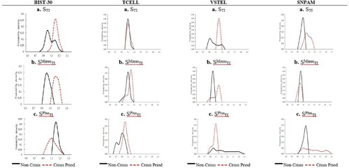
Figure 1. Realised volatility. This table shows realised volatility for BIST-30 and individual stocks in the non-crisis periods and the crisis period. Individual stocks are TCELL, VSTEL and SNPAM, which represent big, medium and small stocks respectively. The data sample ranges from January 1, 2005 to December 31, 2013, including 2,268 trading days. The intraday interval is five minutes. The crisis period considered in this paper is from July 19, 2007 to May 29, 2009.

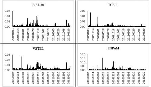
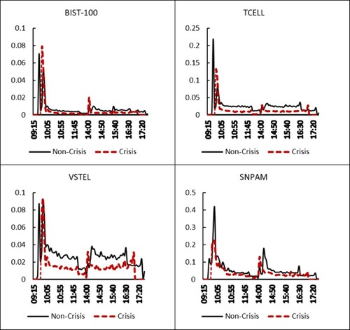
The proportion of significant periodicity-adjusted jumps increases during the crisis period, exceeding that of the non-crisis period, except for SNPAM (small stock). Figure 2 shows that the realised volatility of the emerging market increases just after the opening time in both the morning and the afternoon in both pre-crisis and crisis periods for all cases. It is clear that the most volatile structure happens after the markets’ opening time, and this aspect is little changed between non-crisis and crisis periods. Thus, the descriptive statistics show that the financial crisis has a strong effect on the sitcom prices in terms of jump probability but little on the diurnal volatility characteristics.

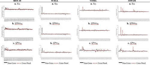
Figure 2. Intraday realised volatility. This table shows intraday realised volatility from 9.15 to 17.40 for BIST-30 and individual stocks in the non-crisis periods and the crisis period. Individual stocks are TCELL, VSTEL and SNPAM, which represent big, medium and small stocks respectively. The data sample ranges from January 1, 2005 to December 31, 2013, including 2,268 trading days. The intraday interval is five minutes. The crisis period considered in this paper is from July 19, 2007 to May 29, 2009.

We present the intraday periodicity-adjusted jump statistic results (see Boudt, Croux, and Laurent 2011 for detailed calculation of jumps statistic) accounting for the periodic pattern in Figure 3. The adjusted jump test detects not much difference between these sub-periods, indicating that there are slightly less intraday jumps during the crisis period for all cases. Moreover, there are more intraday jumps just after the opening time in both the morning and the afternoon in both pre-crisis and crisis periods for all cases.

Figure 3. Intraday periodicity-adjusted jump statistics. This table shows summary statistics of the periodicity-adjusted intraday jump tests of Andersen, Bollerslev, and Diebold (2007b) for BIST-30 and individual stocks in the non-crisis periods and the crisis period. Individual stocks are TCELL, VSTEL and SNPAM, which represent big, medium and small stocks respectively. The data sample ranges from January 1, 2005 to December 31, 2013, including 2,268 trading days. The intraday interval is five minutes. The crisis period considered in this paper is from July 19, 2007 to May 29, 2009.

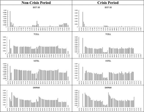
The adjusted jump test detected that around 0.07 of the returns for BIST-30, 0.34 of the returns for TCELL (big stock), 0.31 of the returns for VSTEL (medium stock), and 0.29 of the returns for SNPAM (small stock) are affected by jumps during the non-crisis period, while around 0.04 of the returns for BIST-30, 0.30 of the returns for TCELL (big stock), 0.31 of the returns for VSTEL (medium stock), and 0.28 of the returns for SNPAM (small stock) are affected by jumps during the crisis period.

3.2. Data cleaning and adjustment process

Borsa Istanbul shuts down for a lunch break. This lunch break may introduce a bias in calculating the realised volatility. In order to avoid this bias estimation, the present paper did adjustment of RV estimates for non-trading hours by adding the squared overnight and lunch time returns to RV opentoclose ⁵ (Hansen and Lunde 2005a; Hansen and Lunde 2005b; Hansen and Lunde 2006).

This article followed the steps below for the data cleaning process (see Hansen and Lunde 2006):

• We delete entries with time stamps that lie outside of opening, closing and continuous sessions.

• We delete entries when the price or the volume is zero or negative

• If there are multiple entries per minute, we use the price that has the largest volume

• We delete public holidays (see details for deleted public holidays in Table 2)

• We delete the days when the markets do not trade full days (see Table 2).

• If there were no observations in the dataset based on trading halts, it was filled with the previous price observation.

3.3. Evidence from Brownian motion

We first ask whether the data-generating process has Brownian motion. To answer this question, we compute S_W(p, u_n, kΔ_n) for the sub-sample period. The empirical values of the S_W (p, u_n, kΔ_n) are shown in Figures 4 and 5, where the statistics are calculated for the range of p values from 1 to 1.75 in 0.5 increments, α=2 standard deviation and ω=1/2, k=2. The black solid line and the red dashed line represent non-crisis and crisis periods, respectively. The results of distributions in Fgures 4 and 5 clearly show the presence of Brownian motion in emerging market returns for both non-crisis and crisis periods for all cases. For example, with k=2, p=1, the values of S_W are 1.44 and 1.43 for non-crisis and crisis periods for BIST-30, 1.55 and 1.47 for TCELL (big stock), 1.51 and 1.51 for VSTEL (medium stock), and 1.38 and 1.36 for SNPAM (small stock), respectively, consistent with k^1-p/2.

Figure 4. Sample distribution of S_W statistics. This figure shows the distribution of the non-standardised statistics for Brownian motion given by S_w for BIST-30 and TCELL, which represent the stock market index and big stocks respectively in the non-crisis periods and the crisis period. The table is obtained by computing the S_w, using values of k=2, α=2, and 1≤p≤1.75, taking into account asymmetry effects. The data sample ranges from January 1, 2005 to December 31, 2013, including 2,268 trading days. The intraday interval is five minutes. The crisis period considered in this paper is from July 19, 2007 to May 29, 2009.

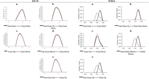
Figure 5. Sample distribution of S_W statistics. This figure shows the distribution of the non-standardised statistics for Brownian motion given by S_w for VSTEL and SNPAM, which represent medium and small stocks respectively in the non-crisis periods and the crisis period. The table is obtained by computing the S_w, using values of k=2, α=2, and 1≤p≤1.75, taking into account asymmetry effects. The data sample ranges from January 1, 2005 to December 31, 2013, including 2,268 trading days. The intraday interval is five minutes. The crisis period considered in this paper is from July 19, 2007 to May 29, 2009.

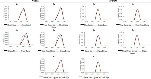
The empirical values of the S_W(p, u_n, kΔ_n), which take into account both the non-crisis/crisis sub-periods and down/up Asymmetry, are shown in panel b to panel e in Figures 4 and 5. The distributions of S_W(p, u_n, kΔ_n) are slightly different, based on the negative and positive movements for both related sub-periods in some cases (see for TCELL (big stock)). Moreover, the Kolmogorov–Smirnov test (see Table 6) shows the existence of different distributions in the crisis and non-crisis periods for some cases; however, the main result does not change and indicates the presence of Brownian motion in emerging market returns in all conditions for all cases.

Thus, the S_W(p, u_n, kΔ_n) statistic does not distinguish between the data of the non-crisis and crisis periods, consistent with the previous findings of the US Treasuries market and the emerging market exchange rate data (Dungey, Holloway, and Yalaman 2012; Dungey, Matei, and Treepongkaruna 2020).

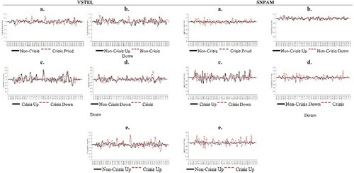
The empirical values of the S_W(p, u_n, kΔ_n), which indicate whether the data-generating process has Brownian motion in the intraday trading period, are shown in Figures 6 and 7, which additionally take into account both non-crisis/crisis sub-periods and down/up asymmetry. The results are consistent with previous findings that indicate evidence of Brownian motion in an intraday trading sample, but in this case it is clear that the presence of the Brownian motion component is not stable during the intraday trading period.

Figure 6. Intraday distribution of S_W statistics. This figure shows the intraday distribution of the non-standardised statistics for Brownian motion given by S_w for BIST-30 and TCELL, which represent the stock market index and big stock respectively in the non-crisis periods and the crisis period. The table is obtained by computing the S_w, using values of k=2, α=2, and 1≤p≤1.75, taking into account asymmetry effects. The data sample ranges from January 1, 2005 to December 31, 2013, including 2,268 trading days. The intraday interval is five minutes. The crisis period considered in this paper is from July 19, 2007 to May 29, 2009.

Figure 7. Intraday distribution of S_W statistics. This figure shows the intraday distribution of the non-standardised statistics for Brownian motion given by S_w for VSTEL and SNPAM, which represent medium and small stocks respectively in the non-crisis periods and the crisis period. The table is obtained by computing the S_w, using values of k=2, α=2, and 1≤p≤1.75, taking into account asymmetry effects. The data sample ranges from January 1, 2005 to December 31, 2013, including 2,268 trading days. The intraday interval is five minutes. The crisis period considered in this paper is from July 19, 2007 to May 29, 2009.

3.4. Evidence from jumps

The empirical values of the S_J(p, ∞, kΔ_n), which indicate whether the data-generating process has jumps, are shown in Figure 8 (panel a) and Figure 9 (panel a), where the statistics are calculated for the range of p values from 2.1 to 6 in 0.1 increments, and k=2. In this case, we calculated the values of the S_J(p, ∞, kΔ_n) without using a truncation level. As indicated before by Aït-Sahalia and Jacod (2012), values of the S_J(p, ∞, kΔ_n) below 1 are indicative of additive noise, or a rounding error dominates the process. Figure 8 (panel a) and Figure 9 (panel a) show that the distribution is largely centred at approximately 1 for the non-crisis period (the median of S_J for the non-crisis period is 0.99, 1.02, 0.88, 0.97 for BIST-30, TCELL (big stock), VSTEL (medium stock) and SNPAM (small stock) respectively), whereas the distribution is slightly larger than 1 for the crisis period (the median of S_J for the crisis period is 1.14, 1.04, 1.07, and 1.14 for BIST-30, TCELL (big stock), VSTEL (medium stock) and SNPAM (small stock) respectively), which supports the presence of a jump in emerging market returns for both sub-samples. This difference indicates that the jumps are less distinguishable from microstructure noise in the non-crisis period. The Kolmogorov–Smirnov test statistic reported in Table 6 shows that this two-sub-sample distribution is not statistically the same. Thus, it is apparent that the S_J(p, ∞, kΔ_n) statistic can be used to distinguish data from non-crisis and crisis periods for emerging market returns. Similar findings are suggested from the US Treasury Market data by Dungey, Holloway, and Yalaman (2012) and from the emerging market exchange rate data by Dungey, Matei, and Treepongkaruna (2020).

Figure 8. Sample distribution of S_j statistics. This figure shows the distribution of the non-standardised statistics for the presence of jumps given by S_j for BIST-30 and TCELL, which represent the stock market index and big stock in the non-crisis periods and the crisis period. The table is obtained by computing the S_j, using values of k=2, α=8, and 2≤p≤6, taking into account asymmetry effects. The data sample ranges from January 1, 2005 to December 31, 2013, including 2,268 trading days. The intraday interval is five minutes. The crisis period considered in this paper is from July 19, 2007 to May 29, 2009.

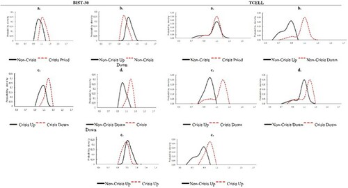
Figure 9. Sample distribution of S_j statistics. This figure shows the distribution of the non-standardised statistics for the presence of jumps given by S_j for VSTEL and SNPAM, which represent medium and small stocks respectively in the non-crisis periods and the crisis period. The table is obtained by computing the S_j, using values of k=2, α=8, and 2≤p≤6, taking into account asymmetry effects. The data sample ranges from January 1, 2005 to December 31, 2013, including 2,268 trading days. The intraday interval is five minutes. The crisis period considered in this paper is from July 19, 2007 to May 29, 2009.

The empirical values of the S_J(p, ∞, kΔ_n), which take into account both non-crisis/crisis periods and down/up asymmetry, are shown in Figure 8 (panel b to panel e) and Figure 9 (panel b to panel e). We support the existence of down/up asymmetry for S_J(p, ∞, kΔ_n) in Figure 8 in all panels for the two sub-sample periods. In other words, the jump intensity is different when the market has a negative or positive return for both sub-periods. In all cases, Table 6 shows the Kolmogorov–Smirnov test statistic, supporting that there is a statistical difference between those two distributions.

For example, for BIST-30, in a non-crisis period, there is a much greater jump intensity if the market has a positive return than if it has negative returns (see Figure 8-panel b). Notably, the results change dramatically in a crisis period, indicating an increase in jump intensity when the market has a negative return compared to when it has a positive return (see Figure 8, panel c). Moreover, if the market has a negative return, it is clear that an increase in jump intensity in a crisis period (see Figure 8, panel d) is consistent with the non-asymmetric effect results (see Figure 8, panel a), whereas there is an increase in jump intensity during the non-crisis period compared to the crisis period when the market has a positive return (see Figure 8, panel e)

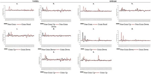
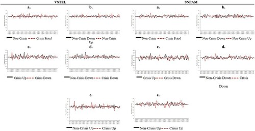
The empirical values of the S_J(p, ∞, kΔ_n) for whether the data-generating process has jumps in the intraday trading period are shown in Figures 10 and 11, which take into account both non-crisis/crisis sub-periods and down/up asymmetry. The results are consistent with previous findings that indicate the presence of the jump component in intraday trading for both sub-sample periods for both BIST-30 and individual stocks. In this case, it is clear that the presence of jumps is not stable during the intraday trading period. Specifically, an increase in jump intensity is clearly seen in both Figures 10 and 11, just after the opening time in both the morning and in the afternoon in all cases.

Figure 10. Intraday distribution of S_j statistics. This figure shows the intraday distribution of the non-standardised statistics for the presence of jumps given by S_j for BIST-30 and TCELL, which represent the stock market index and big stock in the non-crisis periods and the crisis period. The table is obtained by computing the S_j, using values of k=2, α=8, and 2≤p≤6, taking into account asymmetry effects. The data sample ranges from January 1, 2005 to December 31, 2013, including 2,268 trading days. The intraday interval is five minutes. The crisis period considered in this paper is from July 19, 2007 to May 29, 2009.

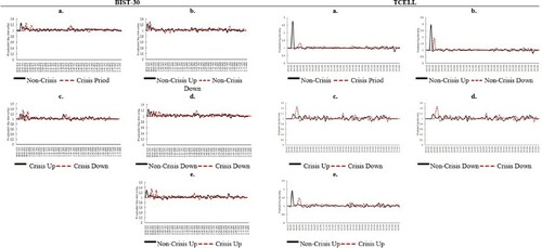
Figure 11. Intraday distribution of S_j statistics. This figure shows the intraday distribution of the non-standardised statistics for the presence of jumps given by S_j for VSTEL and SNPAM, which represent medium and small stocks respectively in the non-crisis periods and the crisis period. The table is obtained by computing the S_j, using values of k=2, α=8, and 2≤p≤6, taking into account asymmetry effects. The data sample ranges from January 1, 2005 to December 31, 2013, including 2,268 trading days. The intraday interval is five minutes. The crisis period considered in this paper is from July 19, 2007 to May 29, 2009.

3.5. Evidence from finite or infinite activity jumps

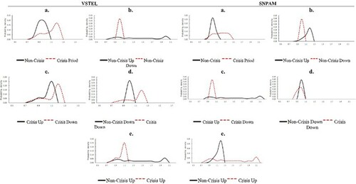
The empirical evidence of S_J(p, ∞, kΔ_n) supports the presence of jumps, but it cannot distinguish whether the jump has finite or infinite activity. Thus, we calculate the statistic of S_FA(p, u_n, kΔ_n), which is similar to S_J(p, ∞, kΔ_n), with additional truncation. The empirical values of the S_FA(p, un, kΔn) are shown in Figure 12 (panel a) and Figure 13 (panel a), where the statistics are calculated for the range of p values from 3 to 6 in 0.1 increments, α=8⁶ and ω=1/2, k=2. The distribution of the calculated test values is centred at approximately 1.5, consistent with finite activity jumps in the non-crisis period.⁷

Figure 12. Sample distribution of S_FA statistics. This figure shows the distribution of the non-standardised statistics that distinguish between finite and infinite jumps given by S_FA for BIST-30 and TCELL, which represent big stocks in the non-crisis periods and the crisis period. The table is obtained by computing the S_FA, using values of k=2, α=8, and 2≤p≤6, taking into account asymmetry effects. The data sample ranges from January 1, 2005 to December 31, 2013, including 2,268 trading days. The intraday interval is five minutes. The crisis period considered in this paper is from July 19, 2007 to May 29, 2009.

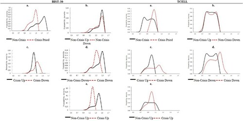
Figure 13. Sample distribution of S_FA statistics. This figure shows the distribution of the non-standardised statistics that distinguish between finite and infinite jumps given by S_FA for VSTEL and SNPAM, which represent medium and small stocks respectively in the non-crisis periods and the crisis period. The table is obtained by computing the S_FA, using values of k=2, α=8, and 2≤p≤6, taking into account asymmetry effects. The data sample ranges from January 1, 2005 to December 31, 2013, including 2,268 trading days. The intraday interval is five minutes. The crisis period considered in this paper is from July 19, 2007 to May 29, 2009.

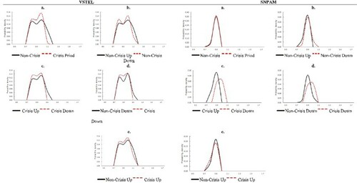
Notably, the distribution of S_FA(p, u_n, kΔ_n) dramatically changes in the crisis period only for BIST-100, rather than individual stocks. The test values of S_FA(p, u_n, kΔ_n) cluster at approximately 1 now, rather than at k^p/2-1, indicating infinite activity jumps. The Kolmogorov–Smirnov test statistic reported in Table 6 shows that the two sub-samples’ distributions are significantly different from one another. Compared to the two sub-sample periods, it is clear that the mass of distributions has shifted to become left-skewed during a crisis period rather than right-skewed during a non-crisis period for BIST-30 only. Thus, it is apparent that the S_FA(p, u_n, kΔ_n) statistic can be used to distinguish data from non-crisis and crisis periods for emerging market index returns. These findings are different from the US Treasury Market data (see Dungey, Holloway, and Yalaman 2012), which show finite jump activity both for non-crisis and crisis periods.

The empirical values of the S_FA(p, u_n, kΔ_n), which take into account both non-crisis/crisis sub-periods and down/up asymmetry, are shown in Figure 12 (panel b to panel e) and Figure 13 (panel b to panel e). We show the existence of down/up asymmetry for S_FA(p, un, kΔn) in most of the panels for the two sub-sample periods. In most of the cases, Table 6 shows that the Kolmogorov–Smirnov test statistic shows statistical differences between those two distributions.

For example, for BIST-100, in the non-crisis period, there are not many differences in down/up asymmetry between non-crisis and crisis periods, indicating the evidence of finite jump activity (see Figure 12, panel b), but notably, the results change in the crisis period. Now, we capture the down/up asymmetry effect. For example, the jumps tend to be finite activity when the price goes up, whereas the jumps tend to be infinite activity when the price goes down (see Figure 12, panel c).

Figure 12 (panel d) and (panel e) shows what happens to S_FA(p, u_n, kΔ_n) statistics if there is down and up asymmetry, respectively; it is clear that the results support a larger infinite jump in activity in the non-crisis period, whereas there is a finite jump in the activity in non-crisis periods for down and up asymmetry.

The empirical values of the S_FA(p, u_n, kΔ_n), which indicate whether the data-generating process has finite or infinite jump activity in the intraday trading period, are shown in Figures 14 and 15, which have already taken into account both the non-crisis/crisis sub-periods and down/up Asymmetry. These results are consistent with previous findings that indicate that the jump activity is not stable during the intraday trading period. Figures 14 and 15 show that there is both finite and infinite jump activity during the intraday period in all cases.

Figure 14. Intraday distribution of S_FA statistics. This figure shows the intraday distribution of the non-standardised statistics that distinguish between finite and infinite jumps given by S_FA for BIST-30 and TCELL, which represent the stock market index and big stocks in the non-crisis periods and the crisis period. The table is obtained by computing the S_FA, using values of k=2, α=8, and 2≤p≤6, taking into account asymmetry effects. The data sample ranges from January 1, 2005 to December 31, 2013, including 2,268 trading days. The intraday interval is five minutes. The crisis period considered in this paper is from July 19, 2007 to May 29, 2009.

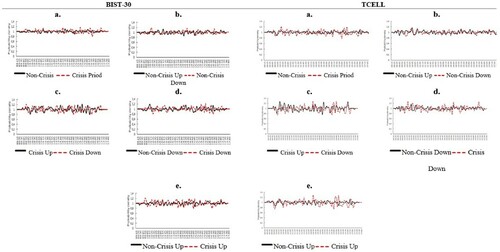
Figure 15. Intraday distribution of S_FA statistics. This figure shows the intraday distribution of the non-standardised statistics that distinguish between finite and infinite jumps given by S_FA for VSTEL and SNPAM, which represent medium and small stocks respectively in the non-crisis periods and the crisis period. The table is obtained by computing the S_FA, using values of k=2, α=8, and 2≤p≤6, taking into account asymmetry effects. The data sample ranges from January 1, 2005 to December 31, 2013, including 2,268 trading days. The intraday interval is five minutes. The crisis period considered in this paper is from July 19, 2007 to May 29, 2009.

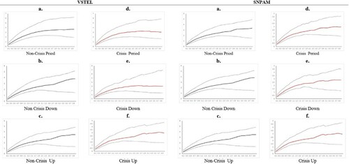
3.6. Evidence from the vibrancy of jump activity

The empirical evidence of the quantile activity signature functions is shown in Figures 16 and 17 for all cases. It is clear that the quantile functions increase for p > 2 for all sub-samples. This emphasises that many of the days in the sample contain jumps at high intensity levels for both non-crisis and crisis periods. The vibrancy of jump activity does not change between non-crisis and crisis periods. Thus, it is apparent that the quantile activity signature function cannot be used to distinguish data from non-crisis and crisis periods for emerging market returns.⁸

Figure 16. Activity signature plots. This figure shows quantile activity signature functions computed for BIST-30 and TCELL, which represent the stock market index and big stock respectively in the non-crisis periods and the crisis period. The table is obtained by computing the function using values of p for the quantiles using 0.25 (for lower bound), 0.50 (for median), and 0.75 for upper bound, taking into account asymmetry effects. The data sample ranges from January 1, 2005 to December 31, 2013, including 2,268 trading days. The intraday interval is five minutes. The crisis period considered in this paper is from July 19, 2007 to May 29, 2009.

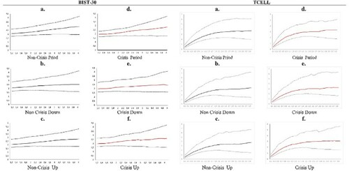
Figure 17. Activity signature plots. This figure shows quantile activity signature functions computed for VSTEL and SNPAM, which represent medium and small stocks respectively in the non-crisis periods and the crisis period. The table is obtained by computing the function using values of p for the quantiles using 0.25 (for lower bound), 0.50 (for median), and 0.75 for upper bound, taking into account asymmetry effects. The data sample ranges from January 1, 2005 to December 31, 2013, including 2,268 trading days. The intraday interval is five minutes. The crisis period considered in this paper is from July 19, 2007 to May 29, 2009.

3.7 Evidence from the relative magnitude of components

The earlier empirical evidence of S_J(p, ∞, kΔ_n) and S_W(p, u_n, kΔ_n) emphasises the presence of both continuous and jump components in emerging market returns. Now, we test what fraction of quadratic variation is attributable to the continuous and jump components for related sub-periods in our sample. We additionally test whether the relative magnitude of the components changes when the market prices go up (up asymmetry effect) or down (down asymmetry effect). The results are shown in Table 5.

Table 5. The proportion of quadratic variation.

	Non-crisis period			Crisis period
	Continuous	Jump		Continuous	Jump
	BIST-30
		Big J.	Small J.		Big J.	Small J.
Non Asymmetry	0.79	0.09	0.12	0.64	0.22	0.14
Up Asymmetry	0.82	0.07	0.11	0.71	0.19	0.10
Down Asymmetry	0.47	0.47	0.08	0.60	0.23	0.17
	TCELL
Non Asymmetry	0.88	0.04	0.08	0.83	0.08	0.09
Up Asymmetry	0.93	0.02	0.05	0.84	0.09	0.07
Down Asymmetry	0.83	0.13	0.04	0.82	0.09	0.09
	VSTEL
Non Asymmetry	0.92	0.05	0.03	0.88	0.08	0.04
Up Asymmetry	0.92	0.02	0.06	0.86	0.05	0.09
Down Asymmetry	0.57	0.41	0.02	0.90	0.04	0.06
	SNPAM
Non Asymmetry	0.70	0.16	0.14	0.74	0.20	0.6
Up Asymmetry	0.71	0.10	0.19	0.75	0.03	0.22
Down Asymmetry	0.53	0.38	0.09	0.73	0.10	0.17

Note: This table shows what fraction of the quadratic variation is attributable to the continuous and jump components for BIST-30 and individual stocks in the non-crisis periods and the crisis period. Individual stocks are TCELL, VSTEL and SNPAM, which represent big, medium and small stocks respectively. This table is obtained by computing the fraction of quadratic variation from the Brownian component, using values of ω=1/2, α=8 and ε=2α. The data sample ranges from January 1, 2005 to December 31, 2013, including 2,268 trading days. The intraday interval is five minutes. The crisis period considered in this paper is from July 19, 2007 to May 29, 2009.

It is clear that the proportion of continuous components decreases more in the crisis period compared with the non-crisis periods, except SNPAM (small stock) (from 0.79 to 0.64 for BIST-30, from 0.88 to 0.83 for TCELL (big stock), and from 0.92 to 0.88 for VSTEL (medium stock)). The same empirical finding is valid for up asymmetry cases (from 0.82 to 0.71 for BIST-30, from 0.93 to 0.84 for TCELL (big stock), and from 0.92 to 0.86 for VSTEL (medium stock)). Interestingly, this situation is the opposite for down asymmetry cases (from 0.47 to 0.60 for BIST-30, from 0.57 to 0.93 for medium, and from 0.53 to 0.73 for SNPAM (small stock)).

The proportion of the large jump component increases in the crisis periods (from 0.09 to 0.22 for BIST-30, from 0.04 to 0.08 for TCELL (big stock), from 0.05 to 0.08 for VSTEL (medium stock), and from 0.16 to 0.20 for SNPAM (small stock)). The same empirical finding is valid for up asymmetry cases periods, except for SNPAM (small stock) (from 0.07 to 0.19 for BIST-30, from 0.02 to 0.09 for TCELL (big stock), and from 0.02 to 0.05 for VSTEL (medium stock)). For down asymmetry cases it decreases from 0.47 to 0.23 for BIST-30, from 0.13 to 0.09 for TCELL (big stock), from 0.41 to 0.04 for VSTEL (medium stock), and from 0.38 to 0.10 for SNPAM (small stock). For the small jump, the proportion increases in the crisis period from 0.12 to 0.14 for BIST-30 and from 0.14 to 0.06 for SNPAM (small stock), while it slightly increases from 0.08 to 0.09 for TCELL (big stock) and 0.03 to 0.04 for VSTEL (medium stock). The empirical finding is quite different for up asymmetry cases for small jumps. It decreases from 0.11 to 0.10 for BIST-30, while it increases from 0.05 to 0.07 for TCELL (big stock), from 0.06 to 0.09 for VSTEL (medium stock), and from 0.09 to 0.17 for SNPAM (small stock). For the down asymmetry cases the range is from 0.08 to 0.17 for BIST-30, from 0.04 to 0.09 for TCELL (big stock), from 0.02 to 0.06 for VSTEL (medium stock), and from 0.09 to 0.17 for SNPAM (small stock).

Thus, it is noticeable that there are very large proportions of large jumps if the market price goes down in the non-crisis periods. In the crisis period, the proportion of large jumps decreases, whereas the proportion of small jumps increases compared to the non-crisis periods. It is apparent that the relative magnitude of components can be used to distinguish the data from non-crisis and crisis periods for emerging market returns.

3.8. Evidence from the tail behaviour

Dungey, Holloway, and Yalaman (2012) proposed the S_TI(p, u_n, kΔ_n) statistic to test the tail behaviour of the distributions, as a simple extension of the set of statistics suggested by Aït-Sahalia and Jacod (2012). It is also possible to test negative and positive tail behaviour using ${\text{S}}_{\text{TI}}^{\text{Minus}}(\text{p, }{\text{u}}_{\text{n}}\text{, k}{\mathrm{\Delta }}_{\text{n}})$ and ${\text{S}}_{\text{TI}}^{\text{Plus}}(\text{p, }{\text{u}}_{\text{n}}\text{, k}{\mathrm{\Delta }}_{\text{n}})$, where the statistics are calculated for the range of p values from 3 to 6 in 0.1 increments, α=8⁹ and ω=1/2, k=2. In the presence of jumps, we report the empirical evidence of S_TI(p, u_n, kΔ_n) and ${\text{S}}_{\text{TI}}^{\text{Minus}}(\text{p, }{\text{u}}_{\text{n}}\text{, k}{\mathrm{\Delta }}_{\text{n}})$ respectively in Figure 18, to show the distinction between small and large jump behaviour in the tail during the two sub-periods. Figure 18 (panel a) and Figure 18 (panel b) indicate that the test values of S_TI(p, u_n, kΔ_n) and ${\text{S}}_{\text{TI}}^{\text{Minus}}(\text{p, }{\text{u}}_{\text{n}}\text{, k}{\mathrm{\Delta }}_{\text{n}})$ slightly cluster at approximately 1 rather than at k^p/2-1, indicating the presence of large jump increases in the non-crisis periods. The mass of distributions shifts to become right-skewed during the crisis period for all cases except TCELL (big stock).

Figure 18. The distribution of S_TI, S^Minus_TI, and S^Plus_TI statistics. This figure shows the distribution of the non-standardised statistics for the presence of large jumps given by S_TI, S^Minus_TI, and S^Plus_TI for TCELL, VSTEL and SNPAM, which represent big, medium and small stocks respectively in the non-crisis periods and the crisis period. The table is obtained by computing the statistics of S_TI, S^Minus_TI, and S^Plus_TI, using values of 2.1≤p≤6, α=2, and k=2. The data sample ranges from January 1, 2005 to December 31, 2013, including 2,268 trading days. The intraday interval is five minutes. The crisis period considered in this paper is from July 19, 2007 to May 29, 2009.

The distribution of S_TI(p, un, kΔn) and ${\text{S}}_{\text{TI}}^{\text{Minus}}(\text{p, }{\text{u}}_{\text{n}}\text{, k}{\mathrm{\Delta }}_{\text{n}})$ is now clustered around k^p/2-1 rather than at 1, indicating the presence of a small jump increase in the crisis period. The Kolmogorov–Smirnov test statistic reported in Table 6 shows that these two sub-samples’ distributions are significantly different from one another. We can conclude that there is an increase of a large jump in the non-crisis period, whereas there are small jump increases in the crisis period. The results change for a positive tail. According to Figure 18 (panel c), the presence of small jumps slightly increases in the non-crisis periods, whereas the presence of large jumps slightly increases in the crisis period for BIST-30 and VSTEL (medium stock). The Kolmogorov–Smirnov test statistic reported in Table 6 shows that the two sub-samples’ distributions are significantly different from one another for ${\text{S}}_{\text{TI}}^{\text{Plus}}(\text{p, }{\text{u}}_{\text{n}}\text{, k}{\mathrm{\Delta }}_{\text{n}})$ for all cases. There are similar findings in the literature; for example, Dungey, Holloway, and Yalaman (2012) and Dungey and Gajurel (2014) show similar tail behaviour for the US Treasury Market and exchange rate data, respectively.

Table 6. The Kolmogorov-Smirnov (KS) test.

	BIST-30	TCELL	VSTEL	SNPAM
Non-Crisis Period-Crisis Period
SJ	3.242 (0.000)	1.789 (0.003)	3.130 (0.000)	3.354 (0.000)
SFA	2.460 (0.000)	0.894 (0.400)	0.671 (0.759)	0.335 (0.998)
SW	0.354 (0.998)	1.945 (0.001)	0.354 (0.998)	1.061 (0.211)
STI	3.130 (0.000)	1.118 (0.164)	3.446 (0.000)	4.472 (0.000)
STI^Minus	4.472 (0.000)	2.907 (0.000)	3.242 (0.000)	4.025 (0.000)
STI^Plus	2.907 (0.000)	3.130 (0.000)	3.355 (0.000)	3.354 (0.000)
Non-Crisis Up-Crisis Down
SJ	4.249 (0.000)	4.025 (0.000)	2.907 (0.000)	3.919 (0.000)
SFA	2.236 (0.000)	1.901 (0.001)	1.230 (0.097)	3.130 (0.000)
SW	0.177 (0.998)	2.121 (0.000)	0.884 (0.415)	2.475 (0.000)
Crisis Up-Crisis Down
SJ	3.354 (0.000)	3.578 (0.000)	2.571 (0.000)	4.137 (0.000)
SFA	3.578 (0.000)	2.571 (0.000)	1.006 (0.263)	3.578 (0.000)
SW	0.354 (0.000)	0.530 (0.941)	0.707 (0.699)	2.474 (0.000)
Non Crisis Down-Crisis Down
SJ	4.471 (0.000)	2.683 (0.000)	3.019 (0.000)	3.801 (0.000)
SFA	2.795 (0.000)	1.789 (0.003)	0.894 (0.400)	2.124 (0.000)
SW	0.177 (0.998)	2.298 (0.000)	0.530 (0.941)	1.591 (0.013)
Non Crisis Up-Crisis Up
SJ	2.683 (0.000)	3.019 (0.000)	3.120 (0.000)	3.354 (0.000)
SFA	3.690 (0.000)	1.342 (0.055)	0.335 (0.998)	1.677 (0.007)
SW	0.176 (0.998)	1.591 (0.013)	0.177 (0.998)	0.354 (0.998)

Note: This table shows the KS results for BIST-30 and individual stocks, taking into account the asymmetry effects. Individual stocks are TCELL, VSTEL and SNPAM, which represent big, medium and small stocks respectively. KS tests whether the distribution of statistics such as S_J S_FA S_W S_TI S_TI^Minus S_TI^Plus for the data-generating process is statistically the same for the related sub-period. If F₁(x) and F₂(x) are the respective cumulative density functions, H0= F₁(x) = F₂(x) H1= F₁(x) ≠ F₂(x). The data sample ranges from January 1, 2005 to December 31, 2013, including 2,268 trading days. The crisis period considered in this paper is from July 19, 2007 to May 29, 2009.

The empirical values of the S_TI(p, un, kΔn), ${\text{S}}_{\text{TI}}^{\text{Plus}}(\text{p, }{\text{u}}_{\text{n}}\text{, k}{\mathrm{\Delta }}_{\text{n}})$, and ${\text{S}}_{\text{TI}}^{\text{Minus}}(\text{p, }{\text{u}}_{\text{n}}\text{, k}{\mathrm{\Delta }}_{\text{n}})$ for the intraday trading period are shown in Figure 19, which additionally takes into account both non-crisis/crisis sub-periods. The results indicate an increase in small jump intensity just after the opening time for BIST-30 and TCELL (big stock) in the morning and in the afternoon for both sub-sample periods; however, the same empirical findings only indicate a valid crisis period for medium and SNPAM (small stock). Additionally, Figure 19 clearly emphasises the evidence of large jumps during the intraday period. Thus, it is evident that the tail behaviour can be used to distinguish data from non-crisis and crisis periods for emerging market returns.

Figure 19. This figure shows the intraday distribution of the non-standardised statistics for the presence of large jumps given by S_TI, S^Minus_TI, and S^Plus_TI for TCELL, VSTEL and SNPAM, which represent big, medium and small stocks respectively in the non-crisis periods and the crisis period. The table is obtained by computing the statistics of S_TI, S^Minus_TI, and S^Plus_TI, using values of 2.1≤p≤6, α=2, and k=2. The data sample ranges from January 1, 2005 to December 31, 2013, including 2,268 trading days. The intraday interval is five minutes. The crisis period considered in this paper is from July 19, 2007 to May 29, 2009.

3.9. Identifying stressful days

Dungey, Matei, and Treepongkaruna (2020) proposed the I_stress,t (p, u_n, kΔ_n) statistic to identify stressful days. The idea is based on the rolling ratio of [S_TI,t(p, u_n, kΔ_n)/ S_TI,t-1(p, u_n, kΔ_n)], the statistic for testing the tail behaviour of the distributions where the statistics are calculated for the range of values p=3,α=8, ω=0.5, k=2 and θ=4.¹⁰

Table 7 shows that there are eight stressful days identified in the crisis period (0.17 percent exceedances for the crisis period) and 14 stressful days identified in the non-crisis period (0.08 percent exceedances for the non-crisis period) for the absolute tail for BIST-30, which is the sum of both positive and negative tails.

Table 7. Stressful days for absolute tail.

2005	2006	2007	2008	2009	2010	2011	2012	2013
BIST-30
16-Feb	12-May		23-Jan			9-Aug		23-May
06-Oct	16-May		28-Jan					4-Jun
	8-Jun		8-Sep					25-Jun
	20-July		15-Sep					22-Aug
	25-July		26-Sep					25-Dec
			6-Oct					31-Dec
			13-Oct
			24-Nov
				TCELL
28-Jan	20-Jan		21-Jan	-		24-Feb		25-Jan
19-Apr	14-Jun		13-Feb			30-Sep
	13-July
				VSTEL
			17-Mar	12-Oct		10-Jan	20-Jan	28-Jun
			6-Oct			18-Apr	14-May	18-Jul
			13-Oct			8-Aug		30-Oct
						11-Aug		31-Dec
				SNPAM
	11-Dec	14-Jun	17-Mar	21-Jan	23-Jun	11-Jul	10-Feb	06-Sep
		15-Oct	21-Oct	29-Jun		27-Sep
			16-Dec

Note: The table reports the stressful days for absolute tail, identified as stressful with the I_stress (p, u_n, k, Δ _n) in the paper, using four standard deviations over the median as the threshold value. Stressful days are detected for BIST-30 and individual stocks. Individual stocks are TCELL, VSTEL and SNPAM, which represent big, medium and small stocks respectively. The data sample ranges from January 1, 2005 to December 31, 2013, including 2,268 trading days. The intraday interval is five minutes. The crisis period considered in this paper is from July 19, 2007 to May 29, 2009.

The stress index can also be calculated for positive and negative tails separately. For BIST-30, Table 8 shows the same results for the positive tail, emphasising that there are five stressful days identified in the crisis period (0.11 percent exceedances for the crisis period) and seven stressful days identified in the non-crisis period (0.04 percent exceedances for the non-crisis period). It is clear that there are more stressful days in the crisis period than in the non-crisis periods for both absolute and positive tails.

Table 8. Stressful days for positive tail.

2005	2006	2007	2008	2009	2010	2011	2012	2013
BIST-30
12-Apr	16-May	30 Apr	24-Jan					4-Jun
20-Oct			8-Sep					25-Jun
			17-Sep					2-Sep
			8-Oct
			24-Nov
				TCELL
28-Jan	20-Jan		23-Jan
19-Apr	15-Mar		27-Feb
	13-Jun		28-Feb
	14-Jun		30 Jul
	05-Oct		23-Oct
	07-Dec
				VSTEL
			13-Oct	05-Jun		11-Aug	10-Jan	18-Jul
							20-Jan	30-Oct
							14-May
				SNPAM
			21-Oct	24-Feb	23-Jun	27-Sep	10-Feb	11-Apr
								06-Sep

Note: The table reports the stressful days for positive tail identified as stressful with the I_stress (p, u_n, k, Δ _n) in the paper, using four standard deviations over the median as the threshold value. Stressful days are detected for BIST-30 and individual stocks. Individual stocks are TCELL, VSTEL and SNPAM, which represent big, medium and small stocks respectively. The data sample ranges from January 1, 2005 to December 31, 2013, including 2,268 trading days. The intraday interval is five minutes. The crisis period considered in this paper is from July 19, 2007 to May 29, 2009.

Notably, Table 9 shows that the proportion of stressful days is not significantly different between crisis and non-crisis periods for the negative tail. There is one stressful day identified in the crisis period (0.02 percent exceedances for the crisis period) and six stressful days identified in the non-crisis periods (0.03 percent exceedances for non-crisis periods).

Table 9. Stressful days for negative tail.

2005	2006	2007	2008	2009	2010	2011	2012	2013
BIST-30
17-Mar	8-Jun		15-Sep			9-Aug		6-Jun
								22-Aug
								25-Dec
				TCELL
02-Feb	08-Mar		28-Jan			24-Feb
23-May	06-Jul		08-May			30-Sep
			03-Oct
			16-Oct
				VSTEL
			23-Jan			18-Apr		25-Dec
			14-Mar			08-Aug		31-Dec
			06-Oct
				SNPAM
	24-Mar	14-Jun	17-Mar	24-Feb	06-Jan	11-Aug
	11-Aug		16-Oct	17-Oct	23-Jun	27-Sep

Note: The table reports the stressful days for negative tail, identified as stressful with the I_stress (p, u_n, k, Δ _n) in the paper, using four standard deviations over the median as the threshold value. Stressful days are detected for BIST-30 and individual stocks. Individual stocks are TCELL, VSTEL and SNPAM, which represent big, medium and small stocks respectively. The data sample ranges from January 1, 2005 to December 31, 2013, including 2,268 trading days. The intraday interval is five minutes. The crisis period considered in this paper is from July 19, 2007 to May 29, 2009.

Thus, the stressful day index can be used to distinguish data from non-crisis and crisis periods for emerging market index returns, particularly for absolute and positive tail behaviour. However, in terms of individual stocks, Table 7 shows that there are two (0.04 percent exceedances for the crisis period), three (0.06 percent exceedances for the crisis period), and four (0.09 percent exceedances for the crisis period) stressful days identified in the crisis period and eight (0.04 percent exceedances for the crisis period), eleven (0.06 percent exceedances for the crisis period), and nine (0.05 percent exceedances for the crisis period) stressful days identified in the non-crisis periods for the absolute tail for TCELL, VSTEL and SNPAM, respectively.

Table 8 shows that there are five (0.11 percent exceedances for the crisis period), one (0.02 percent exceedances for the crisis period), and two (0.04 percent exceedances for the crisis period) stressful days identified in the crisis period and eight (0.04 percent exceedances for the crisis period), seven (0.04 percent exceedances for the crisis period), and five (0.03 percent exceedances for the crisis period) stressful days identified in the non-crisis periods for the positive tail for TCELL,VSTEL and SNPAM, respectively. Finally, Table 9 shows that there are four (0.09 percent exceedances for the crisis period), three (0.06 percent exceedances for the crisis period), and three (0.06 percent exceedances for the crisis period) stressful days identified in the crisis period and six (0.03 percent exceedances for the crisis period), four (0.02 percent exceedances for the crisis period), and eight (0.04 percent exceedances for the crisis period) stressful days identified in the non-crisis periods for the negative tail for TCELL, VSTEL and SNPAM, respectively. We can conclude that the stressful day index can be used to distinguish data from non-crisis and crisis periods for individual stock returns as well (see Tables 7–9).

4. Policy implications

The economic implications of our results are mainly related to optimal portfolio choice, asset pricing, risk management, option pricing and hedging strategies. Our empirical analysis reveals strong evidence of jumps in the stock market data during the crisis period. The presence of jumps in asset returns changes significantly the optimal portfolio allocation. One possible implication of such jumps is to reduce the diversification potential of assets especially in crisis periods.

The evidence for time-variation and commonality of jump risks could potentially have asset-pricing implications and therefore increases in jump risk could require compensation in the form of a risk premium. Risk management is primarily concerned with the tails of the returns’ distributions over different horizons. Ait Aït-Sahalia and Jacod (2012) suggest that analysing tail behaviour of stock returns between crisis and non-crisis period is likely to have risk management implications. For example, the main risk faced by high-frequency traders comes from the small jumps’ component.

It is very important to understand the underlying data generating process of asset return for constructing appropriate option pricing models and our empirical analysis indicates that jumps probably occur more frequently than observed in the option pricing literature, more notably in crisis periods. Therefore, constructing a model that incorporates high levels of jump activity might better be able to explain the empirical characteristics of option prices.

It is well documented in the literature that there are differences in price jump dynamics across stock markets. Hence, investors have to model emerging and developed markets differently to properly reflect their individual dynamics (Dungey, Holloway, and Yalaman 2011, 2020). Another practical policy implication of our empirical findings is that regulators should attempt to design appropriate and efficient early warning systems that would prevent dramatic jumps in financial instrument prices.

5. Conclusions

The way stock market trading is performed has evolved enormously over time as a result of technological advancements. Computing technology in particular has revolutionised the way in which financial assets are traded. Submitting trading orders without immediate human intervention, where computer algorithms make trading decisions at superhuman speed, has become an integral part of financial markets.

Analysing the behaviour of emerging market data, particularly during a financial crisis period, is of great importance to investors, analysts and policymakers. This is the first study to investigate emerging market returns with high-frequency data during one crisis period and two non-crisis periods in terms of both the BIST-30 index and samples of individual stocks. We obtain five-minute high-frequency data from the Turkish Stock Exchange Market to examine the data-generating process of emerging market returns during crisis and non-crisis periods. We also test tail behaviour and how data-generating processes changed during the intraday trading period in both crisis and non-crisis periods. Finally, we examine whether the price asymmetry has a significant effect on the data-generating process of emerging market indices during the related sub-periods.

Our empirical results suggest an increased identification of jumps with infinite activity in the crisis period and a decreased identification of jumps with finite activity in the two non-crisis periods. Interestingly, the activity level of jumps does not differ between two sub-periods for individual stock, whether the stock is big, medium and small.

The proportion of large and small jumps increases during the crisis period, whereas the proportion of Brownian motion decreases during the crisis period. There are few large jumps in the intensity of tail behaviour during the crisis period, whereas there are more in the non-crisis periods. Moreover, price asymmetry plays an important role in detecting the data-generating process of emerging market returns. Specifically, jump and jump activity behave differently when there are positive or negative returns in the market. For example, in a non-crisis period, there is a much greater jump intensity if the market has a positive return than if it has negative returns; notably, the results change dramatically in a crisis period, indicating an increase in jump intensity when the market has a negative return compared to when it has a positive return. The jumps tend to be finite activity when the price goes up, whereas the jumps tend to be infinite activity when the price goes down. We show that the data-generating processes are not stable during the intraday trading period and fluctuate slightly, particularly just after the market opening time in the morning and in the afternoon. Finally, we can conclude that there are many more stressful days in the crisis period than in the non-crisis periods in the Turkish stock market, particularly for absolute and negative tail behaviour. Overall, we empirically demonstrate that many statistical tools can be used to distinguish data among non-crisis and crisis periods for emerging market returns.

Our findings have important practical implications for the promotion of an efficient investment environment, since we demonstrate that price asymmetry plays an important role in detecting the data-generating process of emerging market returns. More specifically, jump activity behaves differently when there are positive or negative returns in the market. The findings of the paper are also important for risk management policies and for the purchase and execution decisions of investors, because we show that the data-generating processes are not stable during the intraday trading period and fluctuate slightly, particularly just after the market opening times in the morning and in the afternoon. These findings could play an important role in the development of enhanced investor protection policies by the Capital Markets Board of Turkey (CMB), which is the regulatory and supervisory authority in charge of the securities markets in the country. In future studies, this paper plans to extend these empirical findings, focusing on individual stock returns rather than general stock market indices. It is interesting to compare the empirical features of the estimated process for both the individual stock return and the general stock market index.

Data availability statement

The data that support the findings of this study are available from the corresponding author upon reasonable request.

Disclosure statement

No potential conflict of interest was reported by the author(s).

Additional information

Funding

Abdullah Yalaman acknowledge supports from an Eskisehir Osmangazi University Research Grant (2019, No: 201917026).

Notes on contributors

Abdullah Yalaman

Abdullah Yalaman is a Professor of Finance at Eskisehir Osmangazi University in Turkey. Abdullah is also a Research Associate at the Center for Economics and Econometrics at Bogazici University in Turkey.

Viktor Manahov

Viktor Manahov holds a PhD in Finance from Newcastle University in the UK. Viktor is currently a Senior Lecturer of Finance at the University of York Management School in the UK.

Notes

1 Contagion effect can be defined as the spread of an economic crisis from one market or region to another, and can occur at either a domestic or international level.

2 For example, if the asset return model with Brownian motion with finite activity jumps, it indicates that the market has relatively rare and large jumps at any time interval. However, if the asset return model with Brownian motion with infinite activity jumps, it indicates that the market has both rare and large jumps and more frequent small jumps at any time interval (Aït-Sahalia and Jacod 2012; Lee and Hannig 2010). We have seen from the empirical evidence in the literature that macro news has caused large and rare jumps, whereas the risk for high-frequency trading strategies is caused by small jumps.

3 Setting ω<1/2 allows us to keep all increments that contain a Brownian motion contribution.

4 There are many approaches in the literature to an optimal sampling regime for different assets (see Andersen Torben et al. 1999; Aït-Sahalia, Mykland, and Zhang 2005). Following Andersen Torben et al. (1999), we propose and illustrate a simple volatility signature plot that may help expose the severity of microstructure bias as the sampling frequency increases. The volatility signature plot stabilises at roughly a 5-minute return sampling interval, which indicates that a high-frequency microstructural effect will also be small after a 5-minute return sampling interval. Thus, the volatility signature plot recommends the use of a sampling interval of a 5-minute return for ISE-30 in Turkey. Ait Aït-Sahalia and Jacod (2012) show how estimated statistics behave when market microstructure noise dominates the process. It is clear that those estimated models do not have microstructure noise in our paper.

5 Hansen and Lunde (2005a, 2005b, 2006) study the adjustment of the RV estimates for non-trading hours in many different papers. They mainly recommend three ways of adjusting the RV estimators in order to incorporate the variance over non-trading hours: (i) scaling of RVopentoclose by using a constant scaling factor; (ii) by adding the squared overnight return to RVopentoclose; and, (iii) by optimally selecting weights to linearly combine the RVopentoclose and the squared overnight return.

6 We report α=8 following the existing literature (Aït-Sahalia and Jacod 2012; Dungey and Gajurel 2014; Erdemlioglu, Laurent, and Neely 2013). The results are not sensitive to α. Those results are consistent for the different values of α, which change from five to 10 standard deviations.

7 For example, with k=2, p=3, α=8, the values of S_FA are 1.21 and 1.14 for non-crisis and crisis periods, respectively, consistent with finite activity jumps in crisis periods and infinite activity jumps in crisis periods.

8 The empirical evidence of the activity signature index β_(0,T], which is clustered around 2 if p≤2 and p if p>2, also shows that the process is continuous with the jump model. The results are consistent with the empirical outcome of both S_J(p,∞,k,Δ_n) and S_w(p,u_n,k,Δ_n).

9 We report α=8 following the existing literature (Aït-Sahalia and Jacod 2012; Dungey and Gajurel 2014; Erdemlioglu, Laurent, and Neely 2013). The results are not sensitive to α. Those results are consistent for the different values of α, which change from five to 10 standard deviations.

10 Eichengreen, Rose, and Wyplosz (1996) appy θ=3, but it is also recommended that θ=4 for high-frequency data (Dungey et al, 2009; Dungey and Gajurel 2014).

References

- Aït-Sahalia, Y., and J. Jacod. 2009a. “Estimating the Degree of Activity of Jumps in High Frequency Data.” Annals of Statistics 37: 2202–2244.
- Aït-Sahalia, Y., and J. Jacod. 2009b. “Testing for Jumps in a Discretely Observed Process.” Annals of Statistics 37: 184–222.
- Aït-Sahalia, Y., and J. Jacod. 2010. “Is Brownian Motion Necessary to Model High Frequency Data?” Annals of Statistics 38: 3093–3128.
- Aït-Sahalia, Y., and J. Jacod. 2011. “Testing Whether Jumps Have Finite or Infinte Activity.” Annals of Statistics 39: 1689–1719.
- Aït-Sahalia, Y., and J. Jacod. 2012. “Analyzing the Spectrum of Asset Returns: Jump and Volatility Components in High Frequency Data.” Journal of Economic Literature 50 (4): 1007–1050.
- Aït-Sahalia, Y., P. Mykland, and L. Zhang. 2005. “How Often to Sample a Continuous-Time Process in the Presence of Market Microstructure Noise.” Review of Financial Studies 18: 351–416.
- Aktas, U. O., and L. Kryzanowski. 2014. “Trade classification accuracy for the BIST.” Journal of International Financial Markets 33: 259–282.
- Aktas, O. U., L. Kryzanowski, and J. Zhang. 2020. “Volatility Spillover Around Price Limits in an Emerging Market.” Finance Research Letters 39: 101610.
- Andersen, T. G., T. Bollerslev, and F. X. Diebold. 2007b. “Roughing it up: Including Jump Components in the Measurement, Modeling, and Forecasting of Return Volatility.” The Review of Economics and Statistics 89 (4): 701–720.
- Andersen, T. G., T. Bollerslev, F. X. Diebold, and C. Vega. 2007. “Real-Time Price Discovery in Stock, Bond and Foreign Exchange Markets.” Journal of International Economics 73: 251–277.
- Andersen Torben, G., Tim Bollerslev, Francis X. Diebold, and Paul Labys. 1999. “Realized Volatility and Correlation.” (Understanding, Optimizing, Using and Forecasting) Manuscript, Northwestern University, Duke University and University of Pennsylvania.
- Barunik, J., and L. Vacha. 2013. “Contagion among Central and Eastern European stock markets during the financial crisis [online].” Accessed December 16, 2020. https://arxiv.org/abs/1309.0491.
- BIS. 2009. “The International Financial Crisis: Timeline, Impact and Policy Responses in Asia and the Pacific.” Technical report, Bank for International Settlements (2009).
- Black, B. 1976. “Studies of Stock Price Volatility Changes.” Proceedings of the 1976 Meetings of the American Statistical Association, Business and Economic Statistics, 177–181.
- Bollerslev, T., T. H. Law, and G. Tauchen. 2008. “Risk, Jumps and Diversification.” Journal of Econometrics 144: 234–256.
- Bollerslev, T., Julia Litvinova, and George Tauchen. 2006. “Leverage and Volatility Feedback Effects in High-Frequency Data.” Journal of Financial Econometrics 4 (3): 353–384.
- Boudt, K., C. Croux, and S. Laurent. 2011. “Robust Estimation of Intraweek Periodicity in Volatility and Jump Detection.” Journal of Empirical Finance 18 (2): 353–367.
- Bowsher, C. G. 2007. “Modelling Security Market Events in Continuous Time: Intensity Based, Multivariate Point Process Models.” Journal of Econometrics 141 (2): 876–912.
- Cashin, P., and C. J. McDermott. 1998. “Testing the Consumption-CAPM in Developing Equity Markets.” International Journal of Finance & Economics 3 (2): 127–141.
- Chow, G. C. 1960. “Tests of Equality Between Sets of Coefficients in two Linear Regressions.” Econometrica: Journal of the Econometric Society 28 (3): 591–605.
- Christie, A. C. 1982. “The Stochastic Behavior of Common Stock Variances-Value, Leverage and Interest Rate Effects.” Journal of Financial Economics 3: 145–166.
- Dungey, M., and D. Gajurel. 2014. “Equity Market Contagion During the Global Financial Crisis: Evidence from the World's Eight Largest Economies.” Economic Systems 38 (2): 161–177.
- Dungey, M., J. Holloway, and A. Yalaman. 2011. “Characterizing Financial Crises Through the Spectrum of High Frequency Data [online].” Accessed December 16, 2020. https://www.semanticscholar.org/paper/Characterizing-fi-nancial-crises-through-the-of-Dungey-Holloway/ee41d1aa37b10352247db8d7ec69e996a710d5a5?p2df.
- Dungey, M., J. Holloway, and A. Yalaman. 2012. “Observing the Crisis: Characterising the Spectrum of Financial Markets With High Frequency Data, 2004-2008.” Manuscript.
- Dungey, M., M. Matei, and S. Treepongkaruna. 2020. “Examining Stress in Asian Currencies: A Perspective Offered by High Frequency Financial Market Data.” Journal of International Financial Markets, Institutions and Money 67: 101200.
- Eichengreen, B., A. Rose, and C. Wyplosz. 1996. “Contagious Currency Crises: First Tests.” Scandinavian Journal of Economics 98: 463–484.
- Ekinci, C., E. Akyildirim, and S. Corbet. 2019. “Analysing the Dynamic Influence of US Macroeconomic News Releases on Turkish Stock Markets.” Finance Research Letters 31: 155–164.
- Ekinci, C., and O. Ersan. 2018. “A new Approach for Detecting High-Frequency Trading from Order and Trade Data.” Finance Research Letters 24: 313–320.
- Erdemlioglu, D., S. Laurent, and C. J. Neely. 2013. “Econometric Modeling of Exchange Rate Volatility and Jumps.” Federal Reserve Bank of St. Louis Working Paper, 2013–2024.
- Erdemlioglu, D., S. Laurent, and C. J. Neely. 2015. “Which Continuous-Time Model is Most Appropriate for Exchange Rates?” Journal of Banking & Finance 61: S256–S268.
- Ferriani, F., and P. Zoi. 2020. “The Dynamics of Price Jumps in the Stock Market: an Empirical Study on Europe and U.S.” European Journal of Finance. doi:10.1080/1351847X.2020.1740288.
- Hanousek, J., and J. Novotnı. 2012. “Price Jumps in Visegrad-Country Stock Markets: An Empirical Analysis.” EmergingMarketsReview 13 (2): 184–201.
- Hansen, P. R., and A. Lunde. 2005a. “A Realized Variance for the Whole day Based on Intermittent High-Frequency Data.” Journal of Financial Econometrics 3 (4): 525–554.
- Hansen, P. R., and A. Lunde. 2005b. “A Forecast Comparison of Volatility Models: Does Anything Beat a GARCH(1,1)?” Journal of Applied Econometrics 20: 873–889.
- Hansen, P. R., and A. Lunde. 2006. “Realized Variance and Market Microstructure Noise.” Journal of Business & Economic Statistics 24 (2): 127–161.
- Huang, X., and G. Tauchen. 2007. “The Relative Contribution of Jumps to Total Price Variance.” Journal of Financial Econometrics 3 (4): 456–499.
- Inci, A. C., and D. Ozenbas. 2017. “Intraday Volatility and the Implementation of a Closing Call Auction at Borsa Istanbul.” Emerging Markets Review 33: 79–89.
- Ito, T., and Y. Hashimoto. 2005. “High-Frequency Contagion of Currency Crises in Asia.” Asian Economic Journal 19 (4): 357–381.
- Lee, S. S., and J. Hannig. 2010. “Detecting Jumps from Ĺevy Jump-Diffusion Processes.” Journal of Financial Economics 96: 271–290.
- NBER. 2010. “Business Cycle Dating Committee Report.” Technical report, National Bureau of Economic Research.
- Özen, E., and M. Tetik. 2019. “Did Developed and Developing Stock Markets React Similarly to Dow Jones During 2008 Crisis?” Frontiers in Applied Mathematics and Statistics. doi:10.3389/fams.2019.00049.
- Rodrik, D. 2009. “Industrial Policy: Don't Ask Why.” East Development Journal 1 (1): 1–29.
- Sensoy, A. 2016. “Commonality in Liquidity: Effects of Monetary Policy and Macroeconomic Announcements.” Finance Research Letters 16: 125–131.
- Sensoy, A. 2017. “Firm Size, Ownership Structure, and Systematic Liquidity Risk: The Case of an Emerging Market.” Journal of Financial Stability 31: 62–80.
- Sensoy, A. 2019. “Commonality in ask-Side vs. bid-Side Liquidity.” Finance Research Letters 28: 198–207.
- Taylor, S. J., and X. Xu. 1997. “The Incremental Volatility Information in one Million Foreign Exchange Quotations.” Journal of Empirical Finance 4 (4): 317–340.
- Tiniç, M., and T. Savaser. 2020. “Political Turmoil and the Impact of Foreign Orders on Equity Prices.” Journal of International Financial Markets, Institutions and Money 65: 101174.
- Todorov, V., and G. Tauchen. 2010. “Activity Signature Functions for High Frequency Data Analysis.” Journal of Econometrics 154: 125–138.
- Voronkova, S. 2004. “Equity Market Integration in Central European Emerging Markets: A Cointegration Analysis with Shifting Regimes.” International Review of Financial Analysis 13 (5): 633–647.