Are cryptos becoming alternative assets?

Abstract

This research provides insights for the separation of cryptocurrencies from other assets. Using dimensionality reduction techniques, we show that most of the variation among cryptocurrencies, stocks, exchange rates, commodities, bonds, and real estate indexes can be explained by the tail, memory and moment factors of their log-returns. By applying various classification methods, cryptocurrencies are categorized as a separate asset class, mainly due to the tail factor. The main result is the complete separation of cryptocurrencies from the other asset types, using the Maximum Variance Components Split method. Additionally, we show that cryptocurrencies tend to exhibit similar characteristics over time and become more distinguished from other asset classes (synchronic evolution).

Keywords:

• Cryptocurrency
• classification
• multivariate analysis
• factor model
• variance components split methods
• synchronic evolution

JEL Classifications:

• C1
• G1

1. Introduction

Cryptocurrencies, seen as new digital currencies, have attracted much attention from investors and academics. A search for ‘cryptocurrencies’ on Google Scholar returns more than 39,000 items, as of 28 April 2021. Most research articles focus on Bitcoin (BTC), as it is considered the first cryptocurrency and has the largest capitalization since its inception; see, for example, Dyhrberg (2016a) and Bariviera et al. (2017). More recently, an extensive literature review on Bitcoin can be found in Corbet et al. (2019), whereas a more technical demonstration of the technology behind the Bitcoin is presented in Berentsen and Schar (2018). Along with this growing popularity, the market capitalization of cryptocurrencies was increasing substantially; the total capitalization of cryptocurrencies market was around US$ 2000 billion as of 28 April 2021, from around US$ 10 billion as of 1 January 2014 (https://coinmarketcap.com).

Despite their growing popularity, there is no widely accepted definition of cryptocurrencies which would allow one to identify them within the existing economic theory (Núñez, Contreras-Valdez, and Franco-Ruiz 2019). In general, cryptocurrencies are defined as ‘digital representations of value, made possible by advances in cryptography and distributed ledger technology (DLT)’ (I.M.F. Treatment of Crypto Assets in Macroeconomic Statistics 2019). A related, ongoing topic of discussion, is the instrument classification of cryptocurrencies in macroeconomic statistics (I.M.F. Treatment of Crypto Assets in Macroeconomic Statistics 2019; Zwijnenburg, De Queljoe, and Ynesta 2020).

Since it appears to be difficult to reach consensus on a standard definition of cryptocurrencies, one can define cryptocurrencies by investigating whether their returns behave similarly to other asset classes (Liu and Tsyvinski 2018).

One of the approaches is to compare cryptocurrencies to classical assets via statistical properties of log-returns distribution. Most of the research shows that cryptocurrencies present long-range memory (Bariviera et al. 2017; Caporale, Gil-Alana, and Plastun 2018; Jiang and Han 2018), multifractality (Takaishi 2018) higher volatility, skewness, and kurtosis compared to classical assets (Klein, Pham Thu, and Walther 2018; Härdle, Harvey, and Reule 2020). Borri (2019) shows that cryptocurrencies exhibit large and volatile return swings and are riskier than most of the other assets, while Zhang et al. (2018) find that cryptocurrencies exhibit heavy tails, quickly decaying returns auto-correlations, slowly decaying auto-correlations for absolute returns, strong volatility clustering, leverage effects, long-range dependence, and power-law correlation between price and volume.

Another approach used to separate cryptocurrencies from classical assets is to develop models able to explain the specificity of cryptocurrencies. For example, Manavi et al. (2020), using the matrix correlation method, compare 7 cryptocurrencies with a sample of three types of monetary systems: 28 exchange rates, 2 commodities, 2 commodity-based indices, and 3 financial market indices. Their results show that the cryptocurrency market and Forex market belong to different system communities.

Using a different approach, Liu and Tsyvinski (2018) analyzed the relationship between cryptocurrencies and each of the following asset classes: stocks, precious metals, and currencies. They show that the risk-return trade-off of three major cryptocurrencies (Bitcoin, Ripple, and Ethereum) is distinct from that of the above asset categories. They also show that the cryptocurrency returns can be predicted by factors which are specific to cryptocurrency markets: momentum and investor attention.

Recently, Liu, Tsyvinski, and Wu (2019) and Liu, Liang, and Cui (2020) developed a three-factor model using the CAPM approach (Fama and French 1996) and showed that the cross-sectional expected cryptocurrency returns can be captured by three factors: the market factor, the size factor and the momentum factor. A similar approach can be found in Shen, Urquhart, and Wang (2020), who developed a three-factor pricing model, consisting of market, size and reversal factors.

In this paper, we provide a classification of the assets' universe, based on which cryptocurrencies pose unique statistical features, allowing their complete separation from classical assets.

Unlike the three-factor model from Liu, Tsyvinski, and Wu (2019), we are using dimensionality reduction techniques (Factor Analysis) applied to a dataset of risk indicators related to the empirical distribution of daily log-returns (following Bariviera et al. 2017; Chan et al. 2017; Caporale, Gil-Alana, and Plastun 2018; Jiang and Han 2018; Takaishi 2018; Klein, Pham Thu, and Walther 2018; Zhang et al. 2018; Borri 2019; Härdle, Harvey, and Reule 2020). We are also using a much larger data set, in terms of the number of assets used, than in Liu, Tsyvinski, and Wu (2019): 234 cryptocurrencies, 635 stocks, 13 exchange rates, 17 commodities, 5 bonds, and 2 real estate indexes. Liu and Tsyvinski (2018) use only 3 cryptocurrencies (Bitcoin, Ripple, and Ethereum), 354 industries in the US, 137 industries in China, 5 exchange rates, and 3 commodities.

A first result of our research is that most of the variation among cryptocurrencies, stocks, exchange rates, commodities, bonds, and real estate indexes can be explained by three factors: the tail factor, the memory factor and the moment factor. These factors are different from the ones obtained in Liu, Tsyvinski, and Wu (2019), Shen, Urquhart, and Wang (2020) or Liu, Liang, and Cui (2020), and allow us to validate the complete separation of cryptocurrencies from other asset types.

The main result of our paper is the complete separation of cryptocurrencies from classical asset types in finance, by using the Maximum Variance Components Split (MVCS) method. The application of other benchmark classification methods (Binary Logistic Regression, Support Vector Machines (SVM), K-means clustering) provides also an almost complete separation. Our results add to the current literature on this topic by showing that the most important factor which differentiates cryptocurrencies from classical assets is the tail behaviour of the log-returns distribution.

Another important result is the discovery of synchronic evolution of cryptocurrencies, compared to classical assets types. Synchronicity refers to the fact that individual cryptocurrencies tend to develop certain similar characteristics over time that make them fully distinguishable from classical assets, i.e. they tend to behave like a homogeneous group, with certain characteristics that individualize them in the assets ecosystem. By using an expanding window approach, we are able to show that cryptocurrencies have a convergent dynamic, which is mainly driven by the tail behaviour of the log-returns distribution. A related analysis can be found in ElBahrawy et al. (2017), where the cryptocurrency market is seen as an evolutive system with several characteristics which are preserved over time.

The importance of the topic analyzed in this study can be defined by three points of interest, depending on the reader's point of view: (i) exploratory interest in the newly arising asset class of cryptocurrencies, as they behave significantly different from the rest of the financial ecosystem; (ii) statistical interest in utilizing existing methodologies for new data, assessing their validity in a high dimensional scope; (iii) Regulatory interest in order to understand which statistical tools are necessary to grasp the major drivers of the new asset class.

This paper is subsequently organized as follows: Section 2 describes the methodology used; Section 3 describes the datasets and interprets the results of the classification; Section 4 describes the synchronic evolution of cryptocurrencies; Section 5 provides a numerical risk example and discuss more on policy implications, while Section 6 concludes. The data and codes used to obtain the results in this paper are available via Quantlet.com.

2. Methodology

The methodology used in this paper has four layers: Layer 1, where we describe the multidimensional dataset used to assess the behaviour of the time series of assets' daily log-returns; Layer 2, where we apply data dimension reduction and orthogonalization methods (Factor Analysis) on the dataset described in Layer 1, to retain the orthogonal factors which maximize the explained variance and could discriminate between cryptocurrencies and classical assets (for some methods using the factors estimated in Layer 2); Layer 3, where we use classification techniques to separate cryptocurrencies from classical assets: Binary Logistic Regression, Support Vector Machine, and K-means clustering applied on the factors estimated in Layer 2 and Maximum Variance Components Split methods applied on the entire dataset; Layer 4, where we confirm the validity of the synchronic evolution property of cryptocurrencies, showing their specific characteristics that differentiate them over time from classical assets, using the projection of the multidimensional dataset described in Layer 1 on the 3D space defined by the factors extracted in Layer 2.

2.1. Layer 1 -- multidimensional dataset

The initial dataset consists of daily log-returns of the assets. To properly classify the assets within the assets universe, we need a dataset of variables-indicators that have the statistical power to differentiate between cryptocurrencies and classical assets (stocks, exchange rates, bonds, real estate and commodities). These indicators are estimates of model parameters associated with the daily log-returns. We denote by n the number of assets in the dataset, by t the time index, $t\in \{1,\dots ,T\}$, where T is the time of the last record in the dataset and by p = 24 is the number of indicators. The daily log-return for asset i in day t, is denoted as $R_{i,t}=\log P_{i,t}-\log P_{i,t-1}$, with $i=1\dots n$, $t=1\dots T$, where $P_{i,t}$ is the closing price for asset i in day t. The dataset of indicators can be seen as a tensor $\mathcal{X}\in {\mathbb{R}}^{n\times p\times T^{\prime }}$, where $T^{\prime }=T-t_0$ is the number of time points. The components of the matrix ${\mathcal{X}}_t=(x_{it,j}{)}_{\begin{array}{c}i=1\dots n\\ j=1\dots p\end{array}}\in {\mathbb{R}}^{n\times p}$, detailed below, are estimates for the time interval $[1,t]$, with $t=t_0,..,T$, where $t_0=[T/3]$ (the integer part of T/3). Most of the variables-indicators used for the taxonomy are selected from the indicators already validated in the literature to differentiate between cryptocurrencies and classical assets.

First, we took into account the central moments of the log-returns distribution, through the following parameters: variance (${\sigma }_{i,t}^2$), skewness ($S_{i,t}$) and Kurtosis ($K_{i,t}$) (used in Bariviera et al. 2017; Härdle, Harvey, and Reule 2020; Takaishi 2018).

Second, we estimated the following parameters of the α-stable distribution, fitted to daily log-returns, to capture heavy tail behaviour: the tail exponent (Stable_${\alpha }_{i,t}\in (0,2]$, with lower values indicating heavier tails) and the scale parameter (Stable_${\gamma }_{i,t}\ge 0$). The α-stable distributions are a well-known class of distributions used in financial modeling (Rachev and Mittnik 2000), capturing the fat tails and the asymmetries of the real-world log-returns distributions (for their use in cryptocurrencies market, see Li et al. 2019; Schnaubelt, Rende, and Krauss 2019; Muvunza 2020). The α-stable parameters were estimated using the empirical characteristic function method, following Koutrouvelis (1980, 1981) and Koutrouvelis and Bauer (1982).

Third, we estimated the quantiles and the conditional tail expectations for the distribution of log-returns, to capture the tail behaviour (Trucíos, Tiwari, and Alqahtani 2020): left-side quantiles $Q_{\alpha ;it}$, right-side quantiles $Q_{1-\alpha ;it}$, conditional left tail expectation $CT{E}_{\alpha ,it}=\mathsf{\text{E}}[R_{it}|R_{it}<Q_{\alpha ;it}]$ and conditional right tail expectation $CT{E}_{1-\alpha ,it}=\mathsf{\text{E}}[R_{it}|R_{it}>Q_{1-\alpha ;it}]$, for $\alpha \in \{0.005,0.01,0.025,0.05\}$. From a market risk perspective, the left tail quantiles can be assimilated to Value-at-Risk, the conditional left tail expectation can be regarded as Expected Shortfall, while the conditional right tail expectation can be seen as the Expected Upside.

Fourth, we estimated a $FIGARCH(1,d,1)$ model, as in Mensi, Al-Yahyaee, and Kang (2019), to capture the long memory effect of volatility. Thus, from the following variance equation of the $FIGARCH(1,d,1)$ model estimated from daily log-returns: (1) ${\sigma }_{it}^2=\omega +[1-\beta L-\varphi L(1-L{)}^{d_{it}}]{ϵ}_{it}^2+\beta {\sigma }_{it-1}^2$(1) where L is the lag operator, we retain in our dataset the estimates of fractional differencing parameter $d_{it}$ (Baillie, Bollerslev, and Mikkelsen 1996).

Fifth, we estimated the first-order auto-correlation coefficient ${\rho }_{it}(1)$ and the Hurst exponent $H_{it}$ of the time series of daily log-returns. The Hurst exponent (Hurst 1951) was estimated based on the discrete second-order derivative in the wavelet domain (Istas and Lang 1997).

In our dataset, the 24 indicators are skewed toward risk measures, which may not fairly justify the role of cryptocurrencies. Similarly to traditional currencies, cryptocurrencies can be used for transaction payment and one can enjoy anonymity in the process of transaction. Although this may be an argument to consider a broader range of indicators, not only from risk measures, the scope of our research scope is to properly separate cryptocurrencies based on the properties of the underlying log-returns distribution.

2.2. Layer 2 -- dimensionality reduction

The most popular methods used to synthesize and extract relevant information from large datasets are Principal Components Analysis (PCA) and Factor Analysis (FA) (Bartholomew 2011). Factor Analysis has been extensively used in cryptocurrencies modeling for classification purposes, e.g. Liu, Tsyvinski, and Wu (2019), who use it to develop the cryptocurrency 3-factor model: the market factor, the size factor and the momentum factor. PCA itself is a linear combination of variables, while FA is a measurement model of a latent variable. The aim of Factor Analysis is to explain the outcome of the p variables of a data matrix using fewer variables, the so-called factors (Härdle and Simar 2019). In our paper, the initial factor pattern is extracted using the principal component method, followed by a Varimax rotation to insure orthogonality of the factors.

2.3. Layer 3 -- separating cryptocurrencies

To separate cryptocurrencies from classical assets, we are using several classification techniques: Binary Logistic Regression, Support Vector Machines, K-means clustering and Maximum Variance Components Split (technical details regarding these techniques can be found in Appendix 1), that can gradually provide complete separation of cryptocurrencies from classical assets. Binary Logistic Regressions have been successfully applied in building statistical arbitrage strategies for cryptocurrencies market (Fischer, Krauss, and Deinert 2019) and to identify and analyze cryptocurrency manipulations in social media (Mirtaheri et al. 2009). Support Vector Machines proved to be a reliable method for price movement prediction of cryptocurrencies (see, for example, Valencia, Gómez-Espinosa, and Valdés-Aguirre 2019 or McNally, Roche, and Caton 2018), while K-means clustering is a classical classification method (MacQueen 1967), which was used in James, Menzies, and Chan (2021) to analyse the impact of Covid-19 on cryptocurrencies market. These methods do not provide complete separation of cryptocurrencies, but they can highlight the main factors that have the ability to discriminate between cryptocurrencies and classical assets. The novelty of our paper is the use of Maximum Variance Component Split methods to completely separate the cryptocurrencies data from the data of other assets. Advantage of MVCS is the unusual analysis of variance with between-group variations only, that depend on the distance between potential clusters and the difference of their means.

2.4. Layer 4 -- synchronic evolution of cryptocurrencies

For observing the synchronic evolution of cryptocurrencies, we are using an expanding window approach, allowing to distinguish the convergence over time of cryptocurrencies. In fact, for $t\in \{t_0,..,T\}$, where $t_0=[T/3]$, the p-dimensional matrix ${\mathcal{X}}_t$ is projected on the 3-dimensional space defined by the tail, memory and moment factors extracted through the Factor Analysis applied on the dataset ${\mathcal{X}}_T$. Looking at the evolution of the Likelihood Ratio from the Logistic Regression model defined in Layer 2, we can observe the ability of the tail factor to discriminate between cryptocurrencies and classical assets. In other words, cryptocurrencies develop over time a similar tail behaviour, pointing out the validity of the synchronic evolution.

3. Data and results

3.1. Multidimensional dataset

The initial dataset consists of daily log-returns of n = 906 assets (cryptocurrencies, commodities, bonds, real estate, exchange rates and stocks -- see Table 1), covering the period 03/01/2014 - 30/11/2020 (1740 trading days). The reason for choosing this time span for the analysis is that before 2014 the liquidity in the cryptocurrency market had been relatively low, their total market capitalization being less than US$16 billion (Feng, Wang, and Zhang 2018). As described in Layer 1 of the methodology, Section 2.1, the multidimensional dataset used for analysis is $\mathcal{X}\in {\mathbb{R}}^{n\times p\times T^{\prime }}$, where n = 906 is the number of assets, p = 24 is the number of indicators, T = 1740 (corresponding to 30/11/2020), $t_0=580$ (corresponding to 22/04/2016) and $T^{\prime }=T-t_0=1160$ is the number of time points. The components of the matrix ${\mathcal{X}}_t=(x_{it,j}{)}_{\begin{array}{c}i=1\dots n\\ j=1\dots p\end{array}}\in {\mathbb{R}}^{n\times p}$, are estimates for the time interval $[1,t]$, with $t=t_0,..,T$.

Table 1. Assets used for analysis.

Type of Asset	Number of Assets	Source
Cryptocurrencies	234	Coinmarketcap
Stocks	635	Bloomberg
Exchange rates	13	Bloomberg
Commodities	17	Bloomberg
Bonds	5	Bloomberg
Real estate	2	Bloomberg

The first component of the dataset¹ consists of a representative sample of 234 cryptocurrencies selected from the top 1000 cryptocurrencies sourced from https://coinmarketcap.com/, accounting for 98% of the total market capitalization, as of 01/12/2020. The cryptocurrencies were selected according to their market capitalization and data availability for at least 750 trading days. The second component consists of a sample of the most traded commodities indexes, the third component consists of a sample of the most liquid exchange rates, the fourth component consists of a sample of bonds, the fifth component consists of two real estate indexes, while the sixth component contains the constituents of the S&P500 Index, Euro Stoxx 50 Index and FTSE 100 Index, recorded at 30/11/2020 (the complete list of assets used in the analysis can be found in Appendix 2). For robustness purposes, only the assets with at least 750 daily historical observations (three trading years) were kept in the analysis. As cryptocurrencies daily data are available at all times, while the classical assets data observe market closure days (weekends and public holidays), the cryptocurrencies data were pre-processed and their closing prices on these particular days were discarded, insuring a homogeneous sample frequency for all assets' types. A detailed analysis regarding data comparability and analysis of cryptocurrencies can be found in Alexander and Dakos (2020).

3.2. Factor analysis

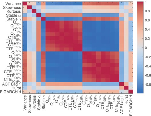
Factor Analysis is a classical method used to find latent variables or factors among observed variables, by grouping variables with similar characteristics. For this purpose, we are using the matrix ${\mathcal{X}}_T=(x_{iT,j}{)}_{\begin{array}{c}i=1\dots n\\ j=1\dots p\end{array}}\in {\mathbb{R}}^{n\times p}$, estimated for the period 03/01/2014 -- 30/11/2020. Three steps are involved: estimation of the correlation matrix for all p = 24 indicators/columns of the matrix ${\mathcal{X}}_T$, shown in Figure 1; extraction of the factors from the correlation matrix, based on the correlation coefficients of the variables; factor rotation, to maximize the relationship between the variables and relevant factors.

Figure 1. Correlation matrix.

SFA_Cryptos

Based on the eigenvalues criteria, three factors were selected, accounting for 88% of the total variance (see Figure 2). In order to test the sampling adequacy of the Factor Analysis, we are using the Kaiser–Meyer–Olkin (KMO) test (Cerny and Kaiser 1977; Kaiser 1974, 1981), which should be greater than 0.5 for a satisfactory Factor Analysis (Tabachnick and Fidell 2013). In our sample, the KMO value is 0.92, pointing out that the Factor Analysis is suitable for structure detection. For the factor rotation, we used the Varimax method, which outputs orthogonal factors, while also minimizing the number of variables that have high loadings on each factor. Based on the rotated factors pattern, the following conclusions can be drawn (see Figure 3):

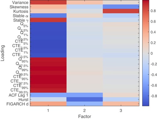
1. First factor: the tail factor, accounting for 76% of the total variance, is highly correlated with the following parameters: the lower and upper quantiles of the distribution of log-returns, the conditional tail expectations, variance, the tail parameter alpha and the scale parameter gamma of the α-stable distribution of log-returns.

2. Second factor: the memory factor, accounting for 6% of the total variance, is highly correlated with the Hurst exponent, the first-order auto-correlation coefficient of log-return and the FIGARCH(1,1) long memory volatility parameter.

3. Third factor: the moment factor, accounting for 6% of the total variance, is highly correlated with the skewness and kurtosis of log-returns distribution.

Figure 2. Scree plot.

SFA_Cryptos

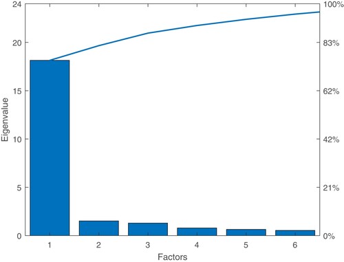
Figure 3. Loadings of the three factors.

SFA_Cryptos

Based on the data revealed in Table 2, one can synthesize few characteristics of cryptocurrencies that differentiate them from the other assets. First, cryptocurrencies have higher variance compared to classical assets, with a scale factor of about 60, on average. Second, as indicated by the values of quantiles and conditional tail expectations, cryptocurrencies have higher propensity for extreme values, in both tails of the log-returns distribution. Third, as indicated by the low values of the alpha-stable tail index, cryptocurrencies log-returns distribution has a larger departure from normality and a higher likelihood for extreme events. These findings extend the results from the literature, for example, Borri (2019), who argues that cryptocurrencies exhibit large and volatile return swings and are riskier than most of the other assets. Fourth, cryptocurrencies exhibit significant negative serial correlation, in line with the results from Griffin and Shams (2020), who documented asymmetric auto-correlations in Bitcoin returns. Fifth, cryptocurrencies have long-term memory, both in log-returns and volatility, as previously shown in related researches (see, for example, Tan, Huang, and Xiao 2021). Sixth, we confirm the results from Momtaz (2021), by showing that cryptocurrencies are the only asset class with substantial positive skewness, so cryptocurrencies have longer left tail of log-returns distribution.

Table 2. Asset classes profile based on the averages of the 24 indicators.

Indicator	Cryptos	Stocks	Bonds	Exchange rates	Commodities	Real Estate
${\sigma }^2\cdot {10}^3$	26.442	0.4	0.745	0.028	0.388	0.146
Skewness	0.686	−0.56	−0.829	−0.937	−0.495	−1.142
Kurtosis	35.163	20.004	35.623	31.949	15.089	17.045
$Stabl{e}_{\alpha }$	1.342	1.602	1.46	1.722	1.662	1.696
$Stabl{e}_{\gamma }$	0.047	0.009	0.009	0.003	0.009	0.006
$Q_{5\mathrm{\%}}$	−0.183	−0.027	−0.029	−0.008	−0.027	−0.018
$Q_{2.5\mathrm{\%}}$	−0.251	−0.038	−0.039	−0.01	−0.036	−0.024
$Q_{1\mathrm{\%}}$	−0.366	−0.054	−0.057	−0.013	−0.05	−0.034
$Q_{0.5\mathrm{\%}}$	−0.485	−0.071	−0.082	−0.015	−0.065	−0.041
$CT{E}_{5\mathrm{\%}}$	−0.308	−0.046	−0.05	−0.011	−0.042	−0.029
$CT{E}_{2.5\mathrm{\%}}$	−0.404	−0.06	−0.066	−0.014	−0.054	−0.038
$CT{E}_{1\mathrm{\%}}$	−0.564	−0.085	−0.097	−0.017	−0.074	−0.052
$CT{E}_{0.5\mathrm{\%}}$	−0.719	−0.106	−0.13	−0.021	−0.091	−0.067
$Q_{95\mathrm{\%}}$	0.19	0.027	0.028	0.008	0.027	0.018
$Q_{97.5\mathrm{\%}}$	0.276	0.036	0.041	0.01	0.035	0.023
$Q_{99\mathrm{\%}}$	0.422	0.051	0.06	0.013	0.05	0.029
$Q_{99.5\mathrm{\%}}$	0.581	0.068	0.078	0.015	0.065	0.034
$CT{E}_{95\mathrm{\%}}$	0.346	0.043	0.051	0.011	0.042	0.026
$CT{E}_{97.5\mathrm{\%}}$	0.467	0.056	0.069	0.013	0.053	0.031
$CT{E}_{99\mathrm{\%}}$	0.662	0.078	0.099	0.017	0.071	0.04
$CT{E}_{99.5\mathrm{\%}}$	0.843	0.095	0.13	0.019	0.085	0.048
$\rho (1)$	−0.116	−0.043	0.15	−0.001	0.024	0.07
Hurst	0.523	0.505	0.569	0.506	0.533	0.49
FIGARCHd	0.553	0.289	0.545	0.407	0.426	0.51

Next, we map cryptocurrencies and classical assets on the 3D space defined by the factors estimated through the Factor Analysis, to derive some clustering effect. Figures 4 and 5 show the assets universe projected onto the 3D space defined by the tail, memory and moment factors; the colour code is the following: green: cryptocurrencies, black: stocks, red: commodities, blue: exchange rates, purple: bonds, yellow: real estate. Moreover, in Figure 4, a $95\mathrm{\%}$ confidence region is estimated for cryptocurrencies, based on the Bivariate Kernel Density. The axis represent the scores estimated for each factor, trough Factor Analysis.

Figure 4. Assets projections on the factors space: (a) tail and memory factors; (b) tail and moment factors.

SFA_Cryptos

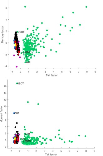
Figure 5. Assets classification: (a) Support Vector Machines; (b) K-means.

SFA_Cryptos

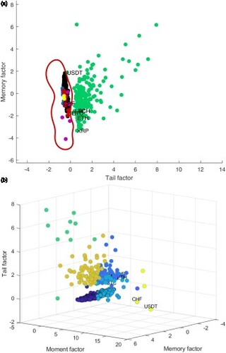
As shown in Figure 4, it appears to be a separation between cryptocurrencies and classical assets, mainly due to the tail and memory factors, while the moment factor is of subliminal importance. The projection on the space defined by the Factor Analysis reveals some cryptocurrencies with atypical behaviour. Thus, Bitcoin (BTC), the oldest and the most traded cryptocurrency, is closer to classical stocks and commodities, i.e. Bitcoin can be considered at the border between the classical assets and cryptocurrencies. This result augments the findings of Dyhrberg (2016b), who concludes that Bitcoin is somewhere in between a currency (USD) and a commodity (Gold). On the other hand, Tether (USDT), a token that attempts to be tied to the US dollar, has a similar profile with the Swiss currency (CHF). Another group of cryptocurrencies (Paxos Standard, TrueUSD, USD Coin, Stasis Euro, Gemini Dollar and sUSD, the so called ‘stable coins’) are closer to exchange rates, from the point of view of the tail factor. These findings build on the results from James, Menzies, and Chan (2021), where Tether (USDT) and TrueUSD (TUSD) are identified as outliers among cryptocurrencies market, using a different data structure, in the context of Covid-19 pandemic.

3.3. Separating cryptocurrencies

In this section, we list the results of the methods presented in Section 2.3. A related question answered is the ability of the factors produced through the Factor Analysis to separate cryptocurrencies from classical assets.

First, for each of the three factors, we estimated the Binary Logistic Regression model (2) $P(Y_i=1)=\frac{\exp ({\beta }_{0j}+{\beta }_{1j}{F}_{ji})}{1+\exp ({\beta }_{0j}+{\beta }_{1j}{F}_{ji})},$(2) where $Y_i=1$ for cryptocurrencies, $Y_i=0$ for classical assets, and $F_j,j\in \{1,2,3\}$ are the orthogonal factors retrieved through the Factor Analysis. Table 3 lists the estimated ${\beta }_{1j}$ of the Binary Logistic Regression model (2(2) $P(Y_i=1)=\frac{\exp ({\beta }_{0j}+{\beta }_{1j}{F}_{ji})}{1+\exp ({\beta }_{0j}+{\beta }_{1j}{F}_{ji})},$(2) ), with the performance measure defined by Equation (A2(A2) ${\tilde{R}}^2=\frac{1-{\left\{\frac{L(\mathbf{0})}{L(\hat{\mathit{\beta }})}\right\}}^{\frac{2}{n}}}{1-\{L(\mathbf{0}){\}}^{\frac{2}{n}}}.$(A2) ).

Table 3. Estimates of binary logistic regression model

Exogenous factor	Tail factor	Moment factor	Memory factor
Estimated ${\beta }_1$	15.450***	−0.738***	0.116
	(4.435)	(0.089)	(0.087)
$\widetilde{R^2}$	0.992	0.122	0.102

Note: Standard errors in parentheses; *** denotes significance at 99% confidence level.

As seen in Table 3, the most important factors regarding the separation between cryptocurrencies and classical assets are the tail factor (having the highest $\widetilde{R^2}$ for the Binary Logistic Regression model) and the memory factor, while the moment factor has no significant influence.

Second, we employed Support Vector Machines on the space defined by the two first factors (tail and moment) and K-means clustering on the 3D space defined on the tail, memory and moment factors (see Figure 5). None of these methods provides complete separation of cryptocurrencies from classical assets, the overall accuracy of the Support Vector Machines non-linear classifier being 99.56%, while the accuracy of the K-means classifier, with 6 clusters, is 98.45%. When using the Support Vector Machines non-linear classifier, the only cryptocurrencies miss-classified are Bitcoin (BTC) and Tether (USDT).

The results when applying the Maximum Variance Component Split (MVCS) method strengthen those of Binary Logistic Regression, Support Vector Machines and K-means clustering, by providing complete separation of cryptocurrencies. The following notation is used: M is the number of positive equidistant angles of [0, π] (we divide [0, π] in M equal intervals and use the intervals' left endpoints as projecting angles), S is a subset of the 24 columns, $N_S$ is the number of projection directions giving perfect classification when S is used, $P_S$ is the percentage of the projection directions examined that provided perfect classification, while $minI,maxI$ are the minimum and the maximum index I value for perfect classification, respectively. The critical value for significance of the I index for $\alpha =5\mathrm{\%}$ and n = 906 is 0.0108. The order of the 24 indicators is as the order of rows in Table 2.

In the following, we present the results of the MVCS method for perfect classification of cryptocurrencies from the other assets. For all five other asset structures (stocks, exchange rates, commodities, bonds and real estate indexes), none of the combinations of M and S examined below provided perfect classification.

Due to processing power constraints, we first split the data in two subsets: the first subset consists of columns/indicators 1–12 of matrix ${\mathcal{X}}_T$ and the second includes columns/indicators 1–12 of matrix ${\mathcal{X}}_T$. For the same reason, projection directions are used only for M = 3, 6 (the number of projection directions used is $M^{d-1}=M^{12-1}=M^{11}$ for each case). Results are shown in Table 4.

Table 4. Results of the MVCS method.

M	S	$N_S$	$P_S$	$minI$	$maxI$
3	1–12	12	0.007$\mathrm{\%}$	0.043	0.096
6	1–12	181618	0.050$\mathrm{\%}$	0.028	0.096
3	13–24	0	0	n/a	n/a
6	13–24	0	0	n/a	n/a

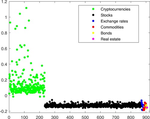
The projection direction that provided the largest index value for columns 1–12 (obtained for M = 6) is: $(-0.062,0,0,-0.108,0.217,-0.433,-0.866,0,0,0,0,0)$. The projected values in this case are shown in Figure 6. As shown in this Figure, the projected values of all cryptocurrencies are greater than the projected values of all other assets, and a vertical hyperplane in the middle of the gap will separate cryptocurrencies from the other assets in the space of the data. Therefore, separation is evident. Also, all 181618 projection directions that achieved perfect classification provided also a statistically significant index values for the normal model.

Figure 6. Projections of a subset of the data (the first 12 indicators) for M = 6 on the projection direction that gave the largest index value among those that gave perfect classification of the cryptocurrencies.

VCS_Cryptos

These results indicate that columns 1–12 are more important for separation of cryptocurrencies than columns 13–24, since only the former confirm separation. Following this, we next applied the MVCS method to columns 1–12, which we further split to columns 1–6 and 7–12. Here, we used $M=3,6,9,12,15$ and 18. For columns 7–12, no $M-$value provided perfect classification for the cryptocurrencies. On the other hand, for columns 1-6 and M = 9, 12, 15 and 18, cryptocurrencies were completely separated from all the other assets; see Table 5. Therefore, we can conclude that the most important columns for complete separation are the first six.

Table 5. Results of the MVCS method, columns 1–6.

M	S	$N_S$	$P_S$	$minI$	$maxI$
3	1–6	0	0	n/a	n/a
6	1–6	0	0	n/a	n/a
9	1–6	19	0.032$\mathrm{\%}$	0.064	0.090
12	1–6	320	0.129$\mathrm{\%}$	0.051	0.099
15	1–6	132	0.017$\mathrm{\%}$	0.055	0.104
18	1–6	1437	0.076$\mathrm{\%}$	0.055	0.1056

Next, the first six indicators/columns are further examined. The MVCS method is applied to all six quintets (each derived by omitting in turn one of the six columns). Higher values of M are used (M = 18, 24 and 32), and the results are reported in Table 6. It can be concluded that the most important indicator/column for perfect separation of cryptocurrencies is the fourth (Stable α), since its omission resulted in not obtaining perfect classification for the cryptocurrencies. The least important among these six columns for separation of cryptocurrencies are Skewness and Kurtosis, since the quintets without these give the largest number of projection directions that provide perfect classification ($N_S$), for all values of M used. Therefore, the corresponding combinations of columns are more suitable for separating the cryptocurrencies from the other assets.

Table 6. Results for cryptocurrencies, all leave-one-out quintets of columns 1–6.

M	S	$N_S$	$P_S$	$minI$	$maxI$
18	1,2,3,4,5	1	0.001$\mathrm{\%}$	0.065	0.065
18	1,2,3,4,6	6	0.006$\mathrm{\%}$	0.057	0.090
18	1,2,3,5,6	0	0	n/a	n/a
18	1,2,4,5,6	213	0.203$\mathrm{\%}$	0.055	0.106
18	1,3,4,5,6	203	0.193$\mathrm{\%}$	0.055	0.106
18	2,3,4,5,6	72	0.069$\mathrm{\%}$	0.066	0.089
24	1,2,3,4,5	0	0	n/a	n/a
24	1,2,3,4,6	9	0.003$\mathrm{\%}$	0.069	0.094
24	1,2,3,5,6	0	0	n/a	n/a
24	1,2,4,5,6	620	0.187$\mathrm{\%}$	0.051	0.106
24	1,3,4,5,6	537	0.162$\mathrm{\%}$	0.051	0.106
24	2,3,4,5,6	192	0.058$\mathrm{\%}$	0.074	0.101
32	1,2,3,4,5	2	0.0002$\mathrm{\%}$	0.065	0.081
32	1,2,3,4,6	21	0.002$\mathrm{\%}$	0.056	0.093
32	1,2,3,5,6	0	0	n/a	n/a
32	1,2,4,5,6	1972	0.188$\mathrm{\%}$	0.050	0.109
32	1,3,4,5,6	1432	0.137$\mathrm{\%}$	0.050	0.109
32	2,3,4,5,6	579	0.055$\mathrm{\%}$	0.059	0.101

Finally, we applied the MVCS code for specific combinations of indicators/columns, in order to further examine the importance of the three factors obtained before (tail, moment and memory). Results for M = 3 are shown² in Table 7.

Table 7. Results of the MVCS method, various indicator combinations, M = 3.

Factor	S	$N_S$	$P_S$
Tail	4–9,14–17	70	0.356$\mathrm{\%}$
Tail and moment	1–9,14–17	80	0.015$\mathrm{\%}$
Left tail and moment	1–9	70	1.070$\mathrm{\%}$
Tail and memory	6–9,14–17,22–24	70	0.119$\mathrm{\%}$
Memory and moment	1–5,22–24	0	0
Tail, memory and moment	1, 4–9, 14–17,22–24	80	0.015$\mathrm{\%}$

From the above, it is further established that tail components are necessary for the separation of cryptocurrencies from the other asserts, since their omission leads to no perfect classification. Another indication is that left tail components seems more important that the corresponding right tail ones. Next, moment components seem to contribute slightly to the perfect classification of cryptocurrencies, whereas memory components do not seem to have any effect on this separation.

We can conclude that cryptocurrencies are financial instruments whose specific difference is the tail behaviour of the distribution of daily log-returns. In other words, based on the tail factor profile, we can conclude that a random asset is likely to be a cryptocurrency if it has the following properties: very long tails of the log-returns distribution (in terms of left and right quantiles and conditional tail expectations), high variance, high value of the α-stable scale parameter and value of the α-stable tail index close to 1.

4. Synchronic evolution of cryptocurrencies

In order to observe the assets dynamics, we are using an expanding window approach, allowing to distinguish the evolution of the clusters. In particular, for $t=t_0,\dots ,T$, the p-dimensional dataset is projected on the k-dimensional space defined by the main factors extracted through the Factor Analysis applied on the matrix ${\mathcal{X}}_T$. By using this projection instead of a time-varying factor model, we are avoiding situations like changes in factors loadings, causing inconsistencies over time.

In the expanding window approach, first, the 24-dimensional dataset is estimated for the time interval $[1,t_0]=$ $[03/01/2014,$ $22/04/2016]$; second, the time window is extended on a daily basis, up to T=30/11/2020 and for each step in time, the dataset is projected on the 2-dimensional space defined by the tail factor and the memory factor, estimated for the entire period.³

Figure 7 presents a snapshot of the evolution of the assets universe using the expanding window approach⁴. Looking at the evolution of the assets universe, it appears that individual cryptocurrencies tend to develop over time similar characteristics (synchronic evolution) that make them fully distinguishable from classical assets. To test this behaviour, we are using the Likelihood Ratio associated to binary logistic model (2(2) $P(Y_i=1)=\frac{\exp ({\beta }_{0j}+{\beta }_{1j}{F}_{ji})}{1+\exp ({\beta }_{0j}+{\beta }_{1j}{F}_{ji})},$(2) ), estimated using the expanding window approach described above. The Likelihood Ratio for this model can be defined as: (3) $LR(\hat{\mathit{\beta }})=-2(\log L(\hat{\mathit{\beta }})-\log L(\widehat{{\mathit{\beta }}_{\mathit{s}}})),$(3) where $L(\widehat{{\mathit{\beta }}_{\mathit{s}}})$ is the maximum likelihood of a saturated model that fits perfectly the sample, while $L(\hat{\mathit{\beta }})$ is the maximum likelihood of the estimated model. In the language of Binary Logistic Regression, the Likelihood Ratio from Equation (3(3) $LR(\hat{\mathit{\beta }})=-2(\log L(\hat{\mathit{\beta }})-\log L(\widehat{{\mathit{\beta }}_{\mathit{s}}})),$(3) ) is called deviance (Hosmer and Lemeshow 2010) and is a measure of model goodness-of-fit, with large values indicating models with poor classification power. The deviance is always positive, being zero only for perfect fit. To derive the statistical significance of the classification, we compare the Likelihood Ratios of the estimated model and of the intercept-only model. Thus, we compute the difference of the likelihood ratios (4) $D=LR(\hat{\mathit{\beta }})-LR(0),$(4) where asymptotically $D\sim {\chi }^2(1)$, $LR(0)$ being the likelihood ratio of the intercept-only model. In fact, we are estimating m models, where $m=T-t_0-1=1161$. For each model, we report the Likelihood Ratio (Figure 8) and the p-value associated to Equation (4(4) $D=LR(\hat{\mathit{\beta }})-LR(0),$(4) ) (see Figure 9). Large p-values indicate that the model might not differ statistically from an intercept-only model.

Figure 7. The evolution of the assets universe using the expanding window approach. The colour code is the following: green -- cryptocurrencies, black -- stocks, red -- commodities, blue -- exchange rates, purple -- bonds, yellow -- real estate.

DFA_Cryptos

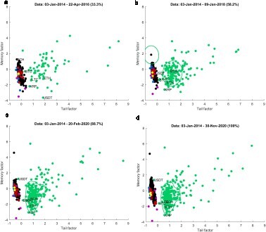
Figure 8. Likelihood Ratios for model (2(2) $P(Y_i=1)=\frac{\exp ({\beta }_{0j}+{\beta }_{1j}{F}_{ji})}{1+\exp ({\beta }_{0j}+{\beta }_{1j}{F}_{ji})},$(2) ), estimated for the period 22/04/2016-30/11/2020, using an expanding window approach.

CONV_Cryptos

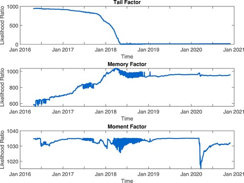
Figure 9. p-values for Equation (4(4) $D=LR(\hat{\mathit{\beta }})-LR(0),$(4) ), estimated for the period 22/04/2016-30/11/2020, using an expanding window approach.

CONV_Cryptos

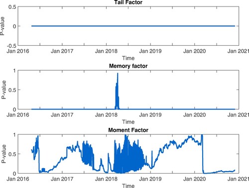
By examining the evolution of the Likelihood Ratios, we can observe a trend change for the tail factor, starting January 2018, when the cryptocurrencies market collapsed after the historical maximum of Bitcoin in December 2017. Thus, the Likelihood Ratio converges to zero, pointing out the ability of the tail factor to discriminate between cryptocurrencies and classical assets. Moreover, as shown by the p-values for the Equation (4(4) $D=LR(\hat{\mathit{\beta }})-LR(0),$(4) ) (see Figure 9), one can conclude that the tail factor can differentiate between cryptocurrencies and classical assets for the entire time-period.

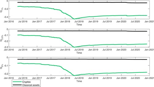
The memory factor lacks significance during the cryptocurrencies crash in January 2018 while the moment factor became significant after February 2020, when the indicators of log-returns distribution for classical assets had a significant shift, capturing the impact of Covid-19 on financial markets. As shown in Figure 10, the variance⁵ and kurtosis of classical assets increased significantly during the Covid-19 period, while the skewness decreased, pointing out that the left tail of log-returns distribution became longer than the right tail, during 2020. As the cryptocurrencies are highly exposed to tail risk, the traditional inference based on normal distribution may became very inappropriate, as illustrated in Figure 11, where the empirical $1\mathrm{\%}$, $2.5\mathrm{\%}$ and $5\mathrm{\%}$ quantiles are plotted for cryptocurrencies and classical assets.

Figure 10. Variance, skewness and kurtosis dynamics by assets class.

CONV_Cryptos

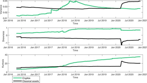
Figure 11. Quantiles dynamics by assets class.

CONV_Cryptos

The most important implication of this analysis is the validity of synchronicity phenomenon among cryptocurrencies: in their evolution, the individual cryptocurrencies have developed similar characteristics (longer tails, higher volatility, higher propensity to extreme returns), that differentiate them from classical assets and position them as a new, different species in the ecosystem of financial instruments. The synchronic evolution of cryptocurrencies can explain their co-jumping behaviour, documented by Bouri, Roubaud, and Shahzad (2020): over time, they tend to behave like a homogeneous group, with certain characteristics that individualize them in the assets ecosystem. Also, our result is in line with the findings from Apergis, Koutmos, and Payne (2021), who proved the convergence in prices for several cryptocurrencies and this convergence behaviour can be driven by changes in market microstructure. A similar conclusion regarding convergence in prices can be found in Papadamou et al. (2021), this convergence being stronger during periods of market growth.

5. Market risk and policy implications

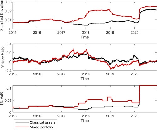
In this section, we provide a numerical risk example, that may be beneficial for practitioners in the field. As the results in Section 3 show that the most important factor separating cryptocurrencies from classical assets is the tail factor, we are investigating the impact of adding cryptocurrencies in a classical assets portfolio, from the point of view of market risk measures like VaR (Value-at-Risk), volatility and Sharpe Ratio. The classical assets portfolio is an equally weighted portfolio constructed using the classical assets in our sample (672 assets, covering the period 03/01/ 2014–30/11/2020), while the mixed portfolio is constructed by adding to the benchmark portfolio all the cryptocurrencies in our sample.

Figure 12 shows the cumulative returns, cumulative standard deviations and cumulative Sharpe Ratios for the classical assets portfolio and the mixed portfolio, computed for the period 03/01/2014-30/11/2020. The portfolio Sharpe Ratio was estimated using the classical formula: $S{R}_p={\mu }_p/{\sigma }_p$, where ${\mu }_p$ and ${\sigma }_p$ are the mean and standard deviation of portfolio returns respectively (Liu and Tsyvinski 2018). The notable impact of adding cryptocurrencies to the classical assets portfolio is a significant increase of volatility and a significant increase in cumulative return until 2019, while the Sharpe Ratios remains stable for the two portfolios. In terms of Value-at-Risk, Figure 13 reports the evolution of Historical Standard deviation, Sharpe ratio and 1% VaR, estimated using a rolling window of w = 250 observations. VaR at significance level α is defined by the following equation: (5) $Pr(r_t<-Va{R}_{\alpha })=\alpha .$(5) As illustrated in this Figure, adding cryptocurrencies in the classical assets portfolio leads to an increased volatility and higher VaR; thus, during the Covid-19 pandemic, the 1% VaR increased from 8% in case of classical assets portfolio to 11% in case of mixed portfolio. At the same time, there is no improvement in the evolution of Sharpe Ratio, as a result of adding cryptocurrencies in the classical assets portfolio. These findings are in line with the results from Naimy, El Chidiac, and El Khoury (2020), who showed that volatility and Value-at-Risk of cryptocurrencies are significantly higher, compared to fiat currencies.

We augment these findings by estimating 1% VaR using several classical methods: Historical VaR, four moment VaR, Normal GARCH(1,1), Student's t GARCH(1,1), Normal GJR-GARCH(1,1,1) and Student's t GJR-GARCH(1,1,1). Historical VaR is estimated as $Va{R}_{\alpha }=-q_{\alpha }$, where $q_{\alpha }$ is the α quantile of the empirical distribution of log-returns. The four moment VaR (proposed by Favre and Galeano 2002 and applied to cryptocurrencies market by Conlon, Corbet, and McGee 2020) is estimated as $MVa{R}_{\alpha }=-({\mu }_p+\hat{Z}(\alpha ,S_p,K_p){\sigma }_p)$, with (6) $\hat{Z}(\alpha ,S_p,K_p)=z_{\alpha }+\frac{1}{6}(z_{\alpha }^2-1)S_p+\frac{1}{24}(z_{\alpha }^3-3z_{\alpha })K_p-\frac{1}{36}(2z_{\alpha }^3-5z_{\alpha })S_p^2.$(6) $z_{\alpha }$ is the α quantile of standard normal distribution, $S_p$ is the portfolio skewness, $K_p$ is the portfolio kurtosis, ${\mu }_p$ and ${\sigma }_p$ are the mean and standard deviation of portfolio returns respectively.

Figure 12. Cumulative average returns, volatility and Sharpe Ratio for classical assets portfolio and the mixed portfolio.

VaR_Cryptos

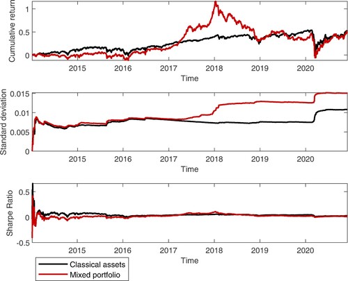
Figure 13. Standard deviation, Sharpe Ratio and Historical 1% VaR for the classical assets portfolio and mixed portfolio, using a rolling window approach.

VaR_Cryptos

The Glosten-Jagannathan-Runkle GARCH (1,1,1) (GJR-GARCH (1,1,1)) model (Glosten, Jagannathan, and Runkle 1993; Zakoian 1994) allows for informational asymmetry in the equation of conditional variance. In GJR-GARCH(1,1,1) model, the log-return is written as $r_t=\mu +{\epsilon }_t$, where μ is the expected return, ${\epsilon }_t={\sigma }_t{z}_t$, $z_t$ are i.i.d. with zero mean (for example, standard Gaussian or Student's t), and the conditional variance follows the equation: (7) ${\sigma }_t^2=\omega +(\alpha +\gamma {\mathbf{1}}_{({\epsilon }_{t-1}>0)}){\epsilon }_{t-1}^2+\beta {\sigma }_{t-1}^2.$(7) For GARCH models, VaR is estimated as $Va{R}_{\alpha }=-({\mu }_p+q_{\alpha }{\sigma }_p)$, where ${\sigma }_p$ is the estimated portfolio conditional volatility, ${\mu }_p$ is the portfolio mean return and $q_{\alpha }$ is the α quantile (standard normal or Student's t). Table 8 reports the average risk exposure, measured through 1% VaR, estimated for the classical assets portfolio, cryptocurrencies only portfolio and mixed portfolio. As shown in this Table, there is a clear difference in average VaR of classical assets portfolio, compared to cryptos only portfolio or to the mixed portfolio. By including cryptocurrencies in the classical assets portfolio, the average 1% VaR may increase from 4.00% to 6.82%, in case of the four moment VaR, and from 2.16% to 3.48% in case of Student's t GJR-GARCH(1,1,1).

Figure 14 shows the estimated Student's t GJR-GARCH(1,1,1) volatility for the classical assets portfolio, cryptocurrencies portfolio and the mixed portfolio. The maximum volatility of cryptocurrencies portfolio is almost 10 times higher than the maximum volatility of the classical assets portfolio, while the maximum volatility of the mixed portfolio is almost three times higher than the maximum volatility of the classical assets portfolio.

Figure 14. Estimated volatilities from Student's t GJR-GARCH(1,1,1) model, using a rolling window approach.

VaR_Cryptos

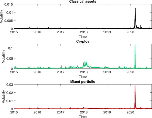
Table 8. Average 1% VaR.

VaR method	Classical assets	Cryptos only	Mixed portfolio
Historical VaR	3.01	16.34	4.37
MVaR	4.00	24.22	6.82
Normal GARCH(1,1)	2.04	12.24	3.21
Student's t GARCH(1,1)	2.22	14.39	3.56
Normal GJR-GARCH(1,1,1)	2.07	12.00	3.11
Student's t GJR-GARCH(1,1,1)	2.16	14.15	3.48

The average 1% VaR is reported in percentage terms; VaR was estimated using a rolling window of 250 trading days, for the period 03/01/2014-30/11/2020.

This result confirms the findings from Naimy et al. (2021), who showed that the most stable cryptocurrency is ten times more volatile than the most unstable fiat currency.

Several implications arise from this exercise and from the findings of our study. First, given cryptocurrencies' unpredictable and highly volatile behaviour, investors may be exposed to higher risks than investing in classical assets. Second, cryptocurrencies can be seen as an alternative for portfolio diversification, if investors are looking for higher compensation from riskier assets (a more in-depth analysis can be found in Naimy, El Chidiac, and El Khoury 2020). Third, as shown in Conlon, Corbet, and McGee (2020), cryptocurrencies may not be suitable for risk-averse investors, especially in bear market circumstances. Because of their high exposure to tail risk, conventional inference based on normal distribution appears to be inappropriate when it comes to the prudential treatment of cryptocurrencies. Furthermore, since the volatility of cryptocurrencies and traditional assets differs by a factor of about 10, cryptocurrencies may require extra attention and monitoring, as their high volatility could jeopardize overall financial stability.

Further research is needed to unveil any theoretical or economical foundation to explain the differences in the statistical properties of cryptos vs. traditional assets. As shown in Giudici, Milne, and Vinogradov (2020), cryptocurrencies are severely affected by uncertainty, arising from two sources: the embedded technology and the ambiguity regarding their fundamental value. Under these conditions, cryptocurrencies would be even more affected by behavioural biases than the classical assets; for example, cryptos may be prone to herding behaviour and bubbles (Cheah and Fry 2015; Papadamou et al. 2021). Technology and market microstructure can explain the convergence behaviour of prices (Apergis, Koutmos, and Payne 2021) and this convergence may facilitate bubble formation. Regarding the fundamental value of cryptocurrencies, most of the researchers agree on the ‘intangible nature of the cryptocurrency value’ (see Giudici, Milne, and Vinogradov 2020). More knowledge on the price dynamics of cryptocurrencies is required to derive the fundamental factors of their statistical behaviour.

6. Conclusions

In this paper, we applied various classification techniques to discriminate between cryptocurrencies and classical assets, like stocks, exchange rates, bonds, real estate indexes, and commodities. Through the means of dimensionality reduction and classification techniques, we proved that most of the variation among cryptocurrencies and classical assets can be explained by three factors: the tail factor, the memory factor and the moment factor. These factors are different from the ones obtained in Liu, Tsyvinski, and Wu (2019) and our analysis revealed that the main difference between cryptocurrencies and classical assets, in terms of properties of the distribution of daily log-returns, is the tail behaviour.

Based on the factors profile, we can conclude that a random asset is likely to be a cryptocurrency if it has the following properties: very long tails of the log-returns distribution (in terms of left and right quantiles and conditional tail expectations), high variance and low values of the α-stable tail parameter, indicating large departure from normality.

Our results provide a series of insights, based on which researchers and practitioners can differentiate cryptocurrencies from classical assets, using the methods presented here. Although classical classification methods (Binary Logistic Regression and Support Vector Machines, K-means clustering) do not provide a complete separation of cryptocurrencies, the Maximum Variance Components Split method achieves this goal.

By looking at the assets universe as a complex ecosystem, we provide empirical evidence that cryptocurrencies exhibit a synchronic evolution, i.e. individual cryptocurrencies develop similar statistical characteristics over time, allowing them to differentiate from classical assets.

From the point of view of the prudential treatment of cryptocurrencies, the traditional inference based on normal distribution seems to be inappropriate, due to their high exposure to tail risk. Moreover, as the volatility of cryptocurrencies is significantly higher then the volatility of classical assets, cryptocurrencies may require special attention and supervision, as their high volatility could have a significant impact on the overall financial stability.

Cryptocurrencies can be seen as digital payment mediums and are also used for speculation. In this research, we are looking at the statistical properties of cryptocurrencies, compared to classical assets; however, this approach can be extended, by including in the analysis some indicators taking into account the payment factors, such as payment techniques, transaction benefits and transaction costs.

Acknowledgments

The authors would like to thank the editor and the anonymous referees for their valuable comments on this article. D. T. Pele would like to thank Dr Lucian Visinescu (Texas State University), for valuable comments and suggestions to improve the quality of the paper. Financial support of the Deutsche Forschungsgemeinschaft's IRTG 1792 grant, the Yushan Scholar Program of Taiwan, the Czech Science Foundation's grant no. 19-28231X / CAS: XDA 23020303 are greatly acknowledged. Y. G. Yatracos would like to thank Professor Dr. Wolfgang K. Härdle and the members of the Ladislaus von Bortkiewicz Chair in Statistics for the warm hosting during his sabbatical, and acknowledges the support of Deutsche Forschungsgemeinschaft's IRTG 1792 grant. All remaining errors are our sole responsibility. The information and views set out in this article are those of the authors and do not necessarily reflect the official opinion of the Central Bank of Cyprus.

Disclosure statement

No potential conflict of interest was reported by the authors.

Additional information

Funding

This research has received funding from the European Union's Horizon 2020 research and innovation program FIN-TECH/825215: A Financial supervision and Technology compliance training programme under the grant agreement No. 825215 (Topic: ICT35-2018, Type of action: CSA). This publication is based upon work from COST Action 19130, supported by COST (European Cooperation in Science and Technology) [COST Action grant CA19130 - FinAI]. Financial support of the Deutsche Forschungsgemeinschaft's IRTG 1792 grant, the Yushan Scholar Program of Taiwan, the Czech Science Foundation's grant no. 19-28231X / CAS: XDA 23020303 are greatly acknowledged. Y. Yatracos acknowledges the support of Deutsche Forschungsgemeinschaft's IRTG 1792 grant.

Notes on contributors

Daniel Traian Pele

Prof. Daniel Traian Pele graduated Mathematics (2000) and got his Master in Stochastic Processes and Theoretical Statistics at the University of Bucharest (2002). He got his Ph.D. in Statistics (2007) and habilitation in Statistics (2019) at the Bucharest University of Economic Studies. He currently serves as a Professor at the Department of Statistics and Econometrics, the Bucharest University of Economic Studies, Romania, teaching Statistics of Financial Markets and Time Series. He is an author of more than 20 scientific publications in internationally refereed journals. The corresponding research profile is that of a data scientist, focused on statistical modelling of financial markets. He was a postdoctoral researcher at ICMA Centre, Reading University, United Kingdom (2011) and a Guest Researcher at Research Data Center from Department of Statistics, Humboldt University from Berlin (2014) and International Research Training Group 1792 “High Dimensional Nonstationary Time Series”, Humboldt University from Berlin (2018, 2019). He is the co-founder of SAS Centre of Excellence in the Bucharest University of Economic Studies (2009), aiming to use SAS as a platform for analytics with applications in economy and finance. He is also a World Bank and European Investment Bank consultant in Romania and he taught courses of Statistics, Econometrics and SAS for the employees of the Romanian National Bank (BNR), National Statistical Institute (INS) and other financial institutions. Publication list can be found at: Google Scholar or ResearchGate.

Niels Wesselhöfft

Dr. Niels Wesselhöfft did his Ph. D. in statistics on “Utilizing self-similar stochastic Processes to model rare Events in Finance” under Prof. Dr. Wolfgang K. Härdle. He is focusing on financial markets, having worked for Deutsche Bank, Veritas Institutional and S-Kreditpartner. His research interests cover robustness in non-stationary environments, high-frequency data and heavy-tailed distributions beyond Gaussianity.

Wolfgang Karl Härdle

Prof. Wolfgang Karl Härdle did 1982 his Dr.rer.nat. in Mathematics at Universität Heidelberg and took his Habilitation at Universität Bonn in 1988. He is Ladislaus von Bortkieviecz chair professor of statistics, Humboldt-Universität zu Berlin. Moreover, he is director of the Sino German International Research Training Group IRTG1792 “High dimensional non stationary time series analysis” (WISE, Xiamen University). His research focuses on dimension reduction techniques, computational statistics and quantitative finance. He has published over 30 books and more than 300 papers in top statistical, econometrics and finance journals, being one of the 1% most ranked researchers on Google Scholar, REPEC and SSRN. He has professional experience in financial engineering, smart data analytics, machine learning and cryptocurrency markets. Innovation: Prof. Hardle has created a financial risk meter FRM and a cryptocurrency index CRIX hu.berlin/frm and a cryptocurrency index CRIX hu.berlin/crix. His web page is: hu.berlin/wkh.

Michalis Kolossiatis

Dr. Michalis Kolossiatis obtained a Bachelor's Degree in Mathematics and Statistics (2003) and a Master's Degree in Statistics (2005) at the University of Cyprus and a PhD in Statistics at the University of Warwick (2009). The PhD Thesis title was “Modelling Via Normalisation for Parametric and Nonparametric Inference” and it was under the guidance of Professors Mark F. J. Steel and Jim E. Griffin. He currently works as a Statistics Officer at the Central Bank of Cyprus. Previous work experience includes: Teaching and Research Fellow at Cyprus University of Technology, Lecturer of Statistics at the University of Kent, UK and at the University of Lancaster, UK, and Visiting Lecturer of Statistics at the University of Cyprus. During his employment at the Universities of Kent and Lancaster, he also served in the Department's Statistical Consultancy Unit. Initially, his research work was mainly on Bayesian nonparametric modelling and density estimation, whereas in the last years, he is more focused on econometric modelling. His main interest in terms of applications is on financial data. He has published articles, among others, in Journal of the Royal Statistical Society (Series B) and Journal of Applied Econometrics. Current research interests consist of: Bayesian nonparametric modelling, density estimation, econometrics and machine learning.

Yannis G. Yatracos

Prof. Yannis G. Yatracos obtained his Ph.D. in Statistics from UC Berkeley under Lucien Le Cam, after the BSc in Math (U. of Athens), MSc in Stat (LSE), DEA and Doctorat de 3eme Cycle in Stat/OR (Paris 6). He is currently Professor of Statistics at Yau Mathematical Sciences Center, Tsinghua University and at BIMSA. Previous regular appointments include the National University of Singapore, Rutgers, Columbia, UC Santa Barbara, University of Montreal and Cyprus U. of Technology. Yannis started his research in density estimation using a Minimum Distance approach, extended the results in non-parametric regression and continued in other areas of Statistics, Mathematical Finance, Matching and in Actuarial Science. He investigated in particular pathologies of plug-in-methods, like the bootstrap and the MLE. His current interests include Learning with Matching, Fiducial ABC, Option Pricing with Le Cam's Experiments, Unmasking in Linear Regression, Cluster and Structures Detection in Big Data. Yannis is IMS and ASA Fellow, Elected ISI member and was Associate of the Society of Actuaries (U.S.A.). His research results have been published, among others, in the Annals of Statistics, JASA, Biometrika, IEEE Transactions on Information Theory, Journal of Classification and Annals of Applied Probability.

Notes

1 The complete list of the assets included in the analysis can be found in the file https://github.com/QuantLet/Genus_proximum_cryptos/blob/master/list.xlsx.

2 Again, this relatively low value of M was used for computational reasons.

3 In this approach, only the first two factors are used, as a 3D evolutionary dynamic would be difficult to read.

4 The daily evolution of the assets universe, for the period 22/04/2016-30/11/2020, is depicted in the video Crypto_movie, attached to this paper as supplementary material.

5 In Figure 10, for classical assets, the variance is multiplied by ${10}^2$.

Appendices

Appendix 1.

Classification methods

Binary logistic regression

The Binary Logistic Regression model quantifies the performance of each of the orthogonal factors extracted through the Factor Analysis to discriminate between cryptocurrencies and classical assets. Thus, we are estimating the following family of models: (A1) $P(Y_i=1)=\frac{\exp ({\beta }_{0j}+{\beta }_{1j}{F}_{ji})}{1+\exp ({\beta }_{0j}+{\beta }_{1j}{F}_{ji})},$(A1) where $Y_i=1$ for cryptocurrencies, $Y_i=0$ for classical assets, and $F_j,j\in \{1,\dots ,k\}$ are the k orthogonal factors retrieved through the Factor Analysis. Based on the explanatory power and the significance of model (A1(A1) $P(Y_i=1)=\frac{\exp ({\beta }_{0j}+{\beta }_{1j}{F}_{ji})}{1+\exp ({\beta }_{0j}+{\beta }_{1j}{F}_{ji})},$(A1) ), we can derive the most important factors contributing to the specific difference of cryptocurrencies. As a performance measure for Model (A1(A1) $P(Y_i=1)=\frac{\exp ({\beta }_{0j}+{\beta }_{1j}{F}_{ji})}{1+\exp ({\beta }_{0j}+{\beta }_{1j}{F}_{ji})},$(A1) ), we are using $\widetilde{R^2}$ (Nagelkerke 1991), where: (A2) ${\tilde{R}}^2=\frac{1-{\left\{\frac{L(\mathbf{0})}{L(\hat{\mathit{\beta }})}\right\}}^{\frac{2}{n}}}{1-\{L(\mathbf{0}){\}}^{\frac{2}{n}}}.$(A2) In Equation (A2(A2) ${\tilde{R}}^2=\frac{1-{\left\{\frac{L(\mathbf{0})}{L(\hat{\mathit{\beta }})}\right\}}^{\frac{2}{n}}}{1-\{L(\mathbf{0}){\}}^{\frac{2}{n}}}.$(A2) ), $L(0)$ is the maximum likelihood of the intercept-only model, $L(\hat{\mathit{\beta }})$ is the maximum likelihood of the full model, and $\hat{\mathit{\beta }}$ is the vector of Maximum Likelihood estimated parameters.

Support vector machines

Support Vector Machines (SVM) is a data classification technique, its goal being to produce a model which predicts target values based on a set of attributes (Cristianini and Shawe-Taylor 2000). The goal is to find a projection that maximizes margin in a hyperplane of the original data, without any parametric assumptions on the underlying stochastic process. The support vectors are determined via a quadratic optimization problem i.e. given a training data set D with n samples and 2 dimensions $D=(X_1,Y_1),\dots (X_n,Y_n)$, $X_i\in {\mathbb{R}}^2,Y_i\in [0,1]$, the aim is to find a hyperplane that maximizes the margin: (A3) $\underset{w,b}{min}\frac{1}{2}\Vert w{\Vert }^2,\mathrm{s}.\mathrm{t}.Y_i(w^{\mathrm{\top }}{X}_i+b)\ge 1,i=1,\dots ,n.$(A3)

K-means clustering algorithm

This clustering method was first popularized by MacQueen (1967), who acknowledged a couple of other researchers that independently used that method around the same time. The aim is to allocate each observation of a data set in one of $k\in \mathbb{N}$ clusters, where k is predefined, so as to minimize the within-cluster sums of squares. In brief, the algorithm proceeds as follows:

1. Take k data points and set them as the cluster centres.

2. Iteratively, for each data point, assign it to the cluster which centre is closer to the data point (the Euclidean distance is usually used, but other distance metrics have been proposed). Update the cluster centre for the selected cluster.

3. Repeat until convergence (i.e. the allocations do not change).

Maximum variance components split methods: MVCS, GMVCS

These methods aim to separate, respectively, the components of a structure like the types of assets herein or the types of Iris flowers, and clusters defined as the components of a mixture distribution. They are based on an unusual variance decomposition in between-group variations (Yatracos 1998, 2013). To describe the sample version of the decomposition, let $X_1,\dots ,X_n$ be i.i.d. random variables. $X_{(j)}$ is the j-th order statistic, $1\le j\le n.$

Consider the groups $X_{(1)},\dots ,X_{(i)}$ and $X_{(i+1)},\dots ,X_{(n)}$ with averages, respectively, ${\overline{X}}_{[1,i]}$ and ${\overline{X}}_{[i+1,n]},$ $i=1,\dots ,n-1,$ then (A4) $\frac{1}{n}\sum _{i=1}^n(X_i-\overline{X}{)}^2=\sum _{i=1}^{n-1}\frac{i(n-i)}{n^2}({\overline{X}}_{[i+1,n]}-{\overline{X}}_{[1,i]})(X_{(i+1)}-X_{(i)}).$(A4) The summands on the right side of Equation (A4(A4) $\frac{1}{n}\sum _{i=1}^n(X_i-\overline{X}{)}^2=\sum _{i=1}^{n-1}\frac{i(n-i)}{n^2}({\overline{X}}_{[i+1,n]}-{\overline{X}}_{[1,i]})(X_{(i+1)}-X_{(i)}).$(A4) ) measure between-groups variations. The standardized sample variance components (A5) $\begin{array}{rl}{W}_i& =W_i(X_1,\dots ,X_n)\end{array}$(A5) (A6) $\begin{array}{rl}& =\frac{i(n-i)}{n}\frac{({\overline{X}}_{[i+1,n]}-{\overline{X}}_{[1,i]})(X_{(i+1)}-X_{(i)})}{\sum _{i=1}^n(X_i-\overline{X}{)}^2},i=1,\dots ,n-1,\end{array}$(A6) indicate the relative contribution of the groups $X_{(1)},\dots ,X_{(i)}$ and $X_{(i+1)},\dots ,X_{(n)}$ in the sample variability. The index (A7) ${\mathcal{I}}_n=max\{W_i,i=1,\dots ,n-1\}$(A7) determines two potential clusters or parts of a structure and is based on averages and inter-point distances. When ${\mathcal{I}}_n=W_j,$ these clusters are ${\tilde{\mathcal{C}}}_1=\{X_{(1)},\dots ,X_{(j)}\},{\tilde{\mathcal{C}}}_2=\{X_{(j+1)},\dots ,X_{(n)}\}.$ The observed ${\mathcal{I}}_n$-value is significant at α-level for the normal model when it exceeds the critical value $[-\ln (-\ln (1-\alpha ))+\ln n]/n$ (Yatracos 2009); $\alpha =0.05$ is used herein.

When $\mathcal{X}$ is the n by r data matrix of r-dimensional observations, ${\mathbf{X}}_j$ is the jth row of $\mathcal{X},j=1,\dots ,n$. The coefficients of the orthogonal projection of $\mathcal{X}$ along the unit norm r-row vector $\mathbf{a}$ are $\mathcal{X}\mathbf{a}=({\mathbf{X}}_1\mathbf{a},\dots ,{\mathbf{X}}_n\mathbf{a})$.

The split in the sorted values of $\mathcal{X}\mathbf{a}$, where (A8) ${\mathcal{I}}_{\mathcal{X}}(\mathbf{a})=max\{W_i({\mathbf{X}}_1\mathbf{a},\dots ,{\mathbf{X}}_n\mathbf{a});i=1,\dots ,n-1\}$(A8) is attained, determines along $\mathbf{a}$ the groups ${\tilde{\mathcal{C}}}_{\mathcal{X},1}(\mathbf{a})$ and ${\tilde{\mathcal{C}}}_{\mathcal{X},2}(\mathbf{a})$ in the $\mathcal{X}$-rows which are potential clusters and parts of a structure. For example, if for the data herein ${\tilde{\mathcal{C}}}_{\mathcal{X},1}(\mathbf{a})$ consists of rows 1-14, cryptocurrencies (a component) among the assets (the structure) are completely separated along $\mathbf{a}.$

The Maximum Variance Component Split (MVCS) method compares known components of a structure, e.g. cryptocurrencies herein, with data splits for a set of unit projection directions ${\mathcal{D}}_M$ usually determined by M positive equidistant angles of $[0,\pi ];$ e.g. when r = 2 and M = 3 the angles used are $\pi /3,2\pi /3,\pi .$ When one of the data split along projection direction $\mathbf{a}$ coincides with a component of the structure we have complete separation of this component along $\mathbf{a}.$

A set of projection directions ${\mathcal{D}}_M$ can be (A9) $({\mathrm{\Pi }}_{l=1}^r\cos {\theta }_l,\sin {\theta }_1{\mathrm{\Pi }}_{l=2}^r\cos {\theta }_l,\dots ,\sin {\theta }_{r-1}\cos {\theta }_r,\sin {\theta }_r),$(A9) where ${\theta }_l$ takes values in $\{\frac{m\pi }{M},m=1,\dots ,M\},l=1,\dots ,r.$

The number of projection directions to be used is $M^{r-1}$. The method is thus computationally intensive for large r and M values, thus it may be used on subsets of the $\mathcal{X}$-columns. The importance of a subset S of $\mathcal{X}$-columns in the separation of a structure's component is measured by the number $N_S$ of projection directions (A9(A9) $({\mathrm{\Pi }}_{l=1}^r\cos {\theta }_l,\sin {\theta }_1{\mathrm{\Pi }}_{l=2}^r\cos {\theta }_l,\dots ,\sin {\theta }_{r-1}\cos {\theta }_r,\sin {\theta }_r),$(A9) ) completely separating the component. Indications for the importance of a specific column c in S in the separation of the same component are obtained by comparing $N_S$ with the number of projection directions $N_{S-c}$ separating the component when c is left out and also by comparing all $N_{S-c},c\in S.$ Similar indications of importance can be used for subgroups of S-columns.

The Global Maximum Variance Component Split (GMVCS) along all projection vectors $\mathcal{D},$ to be obtained from $max\{{\mathcal{I}}_{\mathcal{X}}(\mathbf{a}),\mathbf{a}\in \mathcal{D}\}$, determines two clusters. In practice, its approximation is obtained using ${\mathcal{D}}_M$. The splitting of these clusters may continue (Yatracos 2013).

Appendix 2.

Assets list

Table C1. aaa

Nr.crt.	Name	Type
1	0x	Crypto
2	42-coin	Crypto
3	ALQO	Crypto
4	ATLANT	Crypto
5	Achain	Crypto
6	AdEx Network	Crypto
7	Advanced Internet Blo	Crypto
8	Aeon	Crypto
9	Aeternity	Crypto
10	Agoras Tokens	Crypto
11	Agrello	Crypto
12	Aidos Kuneen	Crypto
13	Aion	Crypto
14	AirSwap	Crypto
15	Alias	Crypto
16	Ambrosus	Crypto
17	Ardor	Crypto
18	Ark	Crypto
19	Autonio	Crypto
20	B2BX	Crypto
21	BLOCKv	Crypto
22	Bancor	Crypto
23	Basic Attention Token	Crypto
24	Bean Cash	Crypto
25	Binance Coin	Crypto
26	BitShares	Crypto
27	Bitcoin	Crypto
28	Bitcoin Cash	Crypto
29	Bitcoin Diamond	Crypto
30	Bitcoin Gold	Crypto
31	Bitcore	Crypto
32	BlackCoin	Crypto
33	Blackmoon	Crypto
34	Blockmason Credit Pro	Crypto
35	Blocknet	Crypto
36	Blox	Crypto
37	Burst	Crypto
38	Bytecoin	Crypto
39	Bytom	Crypto
40	CVCoin	Crypto
41	Carboncoin	Crypto
42	Cardano	Crypto
43	CasinoCoin	Crypto
44	Chainlink	Crypto
45	Change	Crypto
46	Cindicator	Crypto
47	Civic	Crypto
48	Clams	Crypto
49	ColossusXT	Crypto
50	Counterparty	Crypto
51	Credo	Crypto
52	Crown	Crypto
53	CryptoPing	Crypto
54	Cryptonex	Crypto
55	Curecoin	Crypto
56	CyberMiles	Crypto
57	Dash	Crypto
58	Decentraland	Crypto
59	Decred	Crypto
60	DeepOnion	Crypto
61	Dent	Crypto
62	Dentacoin	Crypto
63	Diamond	Crypto
64	DigiByte	Crypto
65	DigitalNote	Crypto
66	DigixDAO	Crypto
67	Dinastycoin	Crypto
68	Dogecoin	Crypto
69	Dragonchain	Crypto
70	Dynamic	Crypto
71	ECC	Crypto
72	EOS	Crypto
73	ERC20	Crypto
74	Einsteinium	Crypto
75	Electroneum	Crypto
76	Enigma	Crypto
77	Ergo	Crypto
78	Ethereum	Crypto
79	Ethereum Classic	Crypto
80	Etheroll	Crypto
81	Everex	Crypto
82	Everus	Crypto
83	FLO	Crypto
84	Factom	Crypto
85	Feathercoin	Crypto
86	Firo	Crypto
87	FirstBlood	Crypto
88	Flash	Crypto
89	FunFair	Crypto
90	GXChain	Crypto
91	GameCredits	Crypto
92	Gas	Crypto
93	Genesis Vision	Crypto
94	Global Cryptocurrency	Crypto
95	Gnosis	Crypto
96	Golem	Crypto
97	Grid+	Crypto
98	GridCoin	Crypto
99	Groestlcoin	Crypto
100	Gulden	Crypto
101	Hellenic Coin	Crypto
102	Hubii Network	Crypto
103	HyperCash	Crypto
104	ICON	Crypto
105	IOTA	Crypto
106	InflationCoin	Crypto
107	Kin	Crypto
108	Komodo	Crypto
109	KuCoin Shares	Crypto
110	Kyber Network	Crypto
111	LATOKEN	Crypto
112	LBRY Credits	Crypto
113	LiteDoge	Crypto
114	Litecoin	Crypto
115	Loopring	Crypto
116	Lykke	Crypto
117	MCO	Crypto
118	MaidSafeCoin	Crypto
119	Maker	Crypto
120	Melon	Crypto
121	Metal	Crypto
122	Metaverse ETP	Crypto
123	Metrix Coin	Crypto
124	MintCoin	Crypto
125	Moeda Loyalty Points	Crypto
126	MonaCoin	Crypto
127	Monero	Crypto
128	Monetha	Crypto
129	Monolith	Crypto
130	Mooncoin	Crypto
131	Myriad	Crypto
132	Mysterium	Crypto
133	NEM	Crypto
134	NULS	Crypto
135	Namecoin	Crypto
136	Nano	Crypto
137	NavCoin	Crypto
138	Neblio	Crypto
139	Nebulas	Crypto
140	Neo	Crypto
141	Nexus	Crypto
142	NoLimitCoin	Crypto
143	NuBits	Crypto
144	NuShares	Crypto
145	Numeraire	Crypto
146	Nxt	Crypto
147	OAX	Crypto
148	OKCash	Crypto
149	OMG Network	Crypto
150	Obyte	Crypto
151	Omni	Crypto
152	PAC Global	Crypto
153	PIVX	Crypto
154	PRIZM	Crypto
155	Particl	Crypto
156	Peercoin	Crypto
157	Phoenix Global	Crypto
158	Phore	Crypto
159	Pillar	Crypto
160	Pluton	Crypto
161	Polybius	Crypto
162	Populous	Crypto
163	PotCoin	Crypto
164	Power Ledger	Crypto
165	Presearch	Crypto
166	Propy	Crypto
167	QASH	Crypto
168	Qtum	Crypto
169	Quantstamp	Crypto
170	Quantum Resistant Led	Crypto
171	Quark	Crypto
172	RChain	Crypto
173	Radium	Crypto
174	Raiden Network Token	Crypto
175	ReddCoin	Crypto
176	Request	Crypto
177	Revain	Crypto
178	Ripio Credit Network	Crypto
179	Rubycoin	Crypto
180	SALT	Crypto
181	SONM	Crypto
182	Safex Token	Crypto
183	SaluS	Crypto
184	Santiment Network Tok	Crypto
185	Shift	Crypto
186	Siacoin	Crypto
187	SingularDTV	Crypto
188	Skycoin	Crypto
189	SmartCash	Crypto
190	SpankChain	Crypto
191	Status	Crypto
192	Stealth	Crypto
193	Steem	Crypto
194	Steem Dollars	Crypto
195	Stellar	Crypto
196	Storj	Crypto
197	Stratis	Crypto
198	Streamr	Crypto
199	SunContract	Crypto
200	Syscoin	Crypto
201	TRON	Crypto
202	TenX	Crypto
203	Tether	Crypto
204	Tezos	Crypto
205	Tierion	Crypto
206	Time New Bank	Crypto
207	ToaCoin	Crypto
208	Ubiq	Crypto
209	Unobtanium	Crypto
210	VIBE	Crypto
211	Verge	Crypto
212	Veritaseum	Crypto
213	Vertcoin	Crypto
214	Viacoin	Crypto
215	Viberate	Crypto
216	Voise	Crypto
217	Voyager Token	Crypto
218	Wagerr	Crypto
219	Waltonchain	Crypto
220	Waves	Crypto
221	Waves Community Token	Crypto
222	WhiteCoin	Crypto
223	Wings	Crypto
224	XRP	Crypto
225	YOYOW	Crypto
226	ZClassic	Crypto
227	Zcash	Crypto
228	ZrCoin	Crypto
229	bitCNY	Crypto
230	district0x	Crypto
231	e-Gulden	Crypto
232	eBitcoin	Crypto
233	iEthereum	Crypto
234	iExec RLC	Crypto
235	3I GROUP PLC ORD 73 19/22P	Stock
236	3M Company	Stock
237	A.O. Smith Corp	Stock
238	ABIOMED Inc	Stock
239	ADIDAS	Stock
240	ADMIRAL GROUP PLC ORD 0.1P	Stock
241	AES Corp	Stock
242	AFLAC Inc	Stock
243	AHOLD DELHAIZE	Stock
244	AIR LIQUIDE	Stock
245	AIRBUS	Stock
246	ALLIANZ	Stock
247	AMADEUS IT GROUP	Stock
248	AMETEK Inc.	Stock
249	ANGLO AMERICAN PLC ORD USD0.5494	Stock
250	ANHEUSER-BUSCH INBEV	Stock
251	ANSYS	Stock
252	ANTOFAGASTA PLC ORD 5P	Stock
253	ASHTEAD GROUP PLC ORD 10P	Stock
254	ASML HLDG	Stock
255	ASSOCIATED BRITISH FOODS PLC ORD	Stock
256	ASTRAZENECA PLC ORD SHS $0.25	Stock
257	AT&T Inc.	Stock
258	AVEVA GROUP PLC ORD 3 5/9P	Stock
259	AVIVA PLC ORD 25P	Stock
260	AXA	Stock
261	AbbVie Inc.	Stock
262	Abbott Laboratories	Stock
263	Accenture plc	Stock
264	Activision Blizzard	Stock
265	Adobe Inc.	Stock
266	Advance Auto Parts	Stock
267	Advanced Micro Devices Inc	Stock
268	Agilent Technologies Inc	Stock
269	Air Products & Chemicals Inc	Stock
270	Akamai Technologies Inc	Stock
271	Alaska Air Group Inc	Stock
272	Albemarle Corp	Stock
273	Alexandria Real Estate Equities	Stock
274	Alexion Pharmaceuticals	Stock
275	Align Technology	Stock
276	Allegion	Stock
277	Alliant Energy Corp	Stock
278	Allstate Corp	Stock
279	Alphabet Inc. (Class C)	Stock
280	Altria Group Inc	Stock
281	Amazon.com Inc.	Stock
282	Amcor plc	Stock
283	Ameren Corp	Stock
284	American Airlines Group	Stock
285	American Electric Power	Stock
286	American Express Co	Stock
287	American International Group	Stock
288	American Tower Corp.	Stock
289	American Water Works Company Inc	Stock
290	Ameriprise Financial	Stock
291	AmerisourceBergen Corp	Stock
292	Amgen Inc.	Stock
293	Amphenol Corp	Stock
294	Analog Devices Inc.	Stock
295	Anthem	Stock
296	Aon plc	Stock
297	Apache Corporation	Stock
298	Apple Inc.	Stock
299	Applied Materials Inc.	Stock
300	Aptiv PLC	Stock
301	Archer-Daniels-Midland Co	Stock
302	Arista Networks	Stock
303	Arthur J. Gallagher & Co.	Stock
304	Assurant	Stock
305	Atmos Energy	Stock
306	AutoZone Inc	Stock
307	Autodesk Inc.	Stock
308	Automatic Data Processing	Stock
309	AvalonBay Communities	Stock
310	Avery Dennison Corp	Stock
311	BAE Systems plc	Stock
312	BARCLAYS PLC ORD 25P	Stock
313	BARRATT DEVELOPMENTS PLC ORD 10P	Stock
314	BASF	Stock
315	BAYER	Stock
316	BCO SANTANDER	Stock
317	BHP Group PLC	Stock
318	BMW	Stock
319	BNP PARIBAS	Stock
320	BP PLC $0.25	Stock
321	BRITISH AMERICAN TOBACCO PLC ORD	Stock
322	BRITISH LAND CO PLC ORD 25P	Stock
323	BT Group plc	Stock
324	BUNZL PLC ORD 32 1/7P	Stock
325	BURBERRY GROUP PLC ORD 0.05P	Stock
326	Baker Hughes Co	Stock
327	Ball Corp	Stock
328	Bank of America Corp	Stock
329	Baxter International Inc.	Stock
330	Becton Dickinson	Stock
331	Berkshire Hathaway	Stock
332	Best Buy Co. Inc.	Stock
333	Bio-Rad Laboratories	Stock
334	Biogen Inc.	Stock
335	BlackRock	Stock
336	Boeing Company	Stock
337	Booking Holdings Inc	Stock
338	BorgWarner	Stock
339	Boston Properties	Stock
340	Boston Scientific	Stock
341	Bristol-Myers Squibb	Stock
342	Broadcom Inc.	Stock
343	Broadridge Financial Solutions	Stock
344	Brown-Forman Corp.	Stock
345	C. H. Robinson Worldwide	Stock
346	CBRE Group	Stock
347	CDW	Stock
348	CF Industries Holdings Inc	Stock
349	CIGNA Corp.	Stock
350	CME Group Inc.	Stock
351	CMS Energy	Stock
352	COCA-COLA HBC AG ORD CHF6.70 (CD	Stock
353	COMPASS GROUP PLC ORD 11 1/20P	Stock
354	CRH	Stock
355	CRH PLC ORD EUR 0.32	Stock
356	CRODA INTERNATIONAL PLC ORD 10.6	Stock
357	CSX Corp.	Stock
358	CVS Health	Stock
359	Cabot Oil & Gas	Stock
360	Cadence Design Systems	Stock
361	Campbell Soup	Stock
362	Capital One Financial	Stock
363	Cardinal Health Inc.	Stock
364	Carmax Inc	Stock
365	Carnival Corp.	Stock
366	Catalent	Stock
367	Caterpillar Inc.	Stock
368	Cboe Global Markets	Stock
369	Celanese	Stock
370	Centene Corporation	Stock
371	CenterPoint Energy	Stock
372	Cerner	Stock
373	Charles Schwab Corporation	Stock
374	Charter Communications	Stock
375	Chevron Corp.	Stock
376	Chipotle Mexican Grill	Stock
377	Chubb Limited	Stock
378	Church & Dwight	Stock
379	Cincinnati Financial	Stock
380	Cintas Corporation	Stock
381	Cisco Systems	Stock
382	Citigroup Inc.	Stock
383	Citizens Financial Group	Stock
384	Citrix Systems	Stock
385	Coca-Cola Company	Stock
386	Cognizant Technology Solutions	Stock
387	Colgate-Palmolive	Stock
388	Comcast Corp.	Stock
389	Comerica Inc.	Stock
390	Conagra Brands	Stock
391	Concho Resources	Stock
392	ConocoPhillips	Stock
393	Consolidated Edison	Stock
394	Constellation Brands	Stock
395	Copart Inc	Stock
396	Corning Inc.	Stock
397	Costco Wholesale Corp.	Stock
398	Crown Castle International Corp.	Stock
399	Cummins Inc.	Stock
400	D. R. Horton	Stock
401	DAIMLER	Stock
402	DANONE	Stock
403	DCC PLC ORD EUR0.25	Stock
404	DEUTSCHE BOERSE	Stock
405	DEUTSCHE POST	Stock
406	DEUTSCHE TELEKOM	Stock
407	DIAGEO PLC ORD 28 101/108P	Stock
408	DTE Energy Co.	Stock
409	DXC Technology	Stock
410	DaVita Inc.	Stock
411	Danaher Corp.	Stock
412	Darden Restaurants	Stock
413	Deere & Co.	Stock
414	Delta Air Lines Inc.	Stock
415	Dentsply Sirona	Stock
416	Devon Energy	Stock
417	DexCom	Stock
418	Diamondback Energy	Stock
419	Digital Realty Trust Inc	Stock
420	Discover Financial Services	Stock
421	Discovery Inc. (Class A)	Stock
422	Dish Network	Stock
423	Dollar General	Stock
424	Dollar Tree	Stock
425	Dominion Energy	Stock
426	Domino's Pizza	Stock
427	Dover Corporation	Stock
428	DuPont de Nemours Inc	Stock
429	Duke Energy	Stock
430	Duke Realty Corp	Stock
431	ENEL	Stock
432	ENGIE	Stock
433	ENI	Stock
434	ENTAIN PLC ORD EUR0.01	Stock
435	EOG Resources	Stock
436	ESSILORLUXOTTICA	Stock
437	EVRAZ plc	Stock
438	EXPERIAN PLC ORD USD0.10	Stock
439	Eastman Chemical	Stock
440	Eaton Corporation	Stock
441	Ecolab Inc.	Stock
442	Edison Int'l	Stock
443	Edwards Lifesciences	Stock
444	Electronic Arts	Stock
445	Emerson Electric Company	Stock
446	Entergy Corp.	Stock
447	Equifax Inc.	Stock
448	Equinix	Stock
449	Equity Residential	Stock
450	Essex Property Trust Inc.	Stock
451	Estee Lauder Companies	Stock
452	Etsy	Stock
453	Everest Re Group Ltd.	Stock
454	Evergy	Stock
455	Eversource Energy	Stock
456	Exelon Corp.	Stock
457	Expedia Group	Stock
458	Expeditors	Stock
459	Extra Space Storage	Stock
460	Exxon Mobil Corp.	Stock
461	F5 Networks	Stock
462	FERGUSON PLC ORD 10P	Stock
463	FLIR Systems	Stock
464	FLUTTER ENTERTAINMENT	Stock
465	FMC Corporation	Stock
466	FRESNILLO PLC ORD USD0.50	Stock
467	Facebook Inc.	Stock
468	Fastenal Co	Stock
469	FedEx Corporation	Stock
470	Federal Realty Investment Trust	Stock
471	Fidelity National Information Se	Stock
472	Fifth Third Bancorp	Stock
473	First Republic Bank	Stock
474	FirstEnergy Corp	Stock
475	Fiserv Inc	Stock
476	FleetCor Technologies Inc	Stock
477	Flowserve Corporation	Stock
478	Flutter Entertainment PLC	Stock
479	Ford Motor Company	Stock
480	Fortinet	Stock
481	Fortive Corp	Stock
482	Fortune Brands Home & Security	Stock
483	Franklin Resources	Stock
484	Freeport-McMoRan Inc.	Stock
485	GLAXOSMITHKLINE PLC ORD 25P	Stock
486	GLENCORE PLC ORD USD0.01	Stock
487	Gap Inc.	Stock
488	Garmin Ltd.	Stock
489	Gartner Inc	Stock
490	General Dynamics	Stock
491	General Electric	Stock
492	General Mills	Stock
493	General Motors	Stock
494	Genuine Parts	Stock
495	Gilead Sciences	Stock
496	Global Payments Inc.	Stock
497	Globe Life Inc.	Stock
498	Goldman Sachs Group	Stock
499	Grainger (W.W.) Inc.	Stock
500	HALMA PLC ORD 10P	Stock
501	HCA Healthcare	Stock
502	HIKMA PHARMACEUTICALS PLC ORD SH	Stock
503	HOMESERVE PLC ORD 2 9/13P	Stock
504	HP Inc.	Stock
505	HSBC HLDGS PLC ORD $0.50 (UK REG	Stock
506	Halliburton Co.	Stock
507	Hanesbrands Inc	Stock
508	Hartford Financial Svc.Gp.	Stock
509	Hasbro Inc.	Stock
510	Healthpeak Properties	Stock
511	Henry Schein	Stock
512	Hess Corporation	Stock
513	Hewlett Packard Enterprise	Stock
514	Hilton Worldwide Holdings Inc	Stock
515	HollyFrontier Corp	Stock
516	Hologic	Stock
517	Home Depot	Stock
518	Honeywell Int'l Inc.	Stock
519	Hormel Foods Corp.	Stock
520	Host Hotels & Resorts	Stock
521	Howmet Aerospace	Stock
522	Humana Inc.	Stock
523	Huntington Bancshares	Stock
524	Huntington Ingalls Industries	Stock
525	IBERDROLA	Stock
526	IDEX Corporation	Stock
527	IDEXX Laboratories	Stock
528	IHS Markit Ltd.	Stock
529	IMPERIAL BRANDS PLC ORD 10P	Stock
530	INFORMA PLC ORD 0.1P	Stock
531	ING GRP	Stock
532	INTERCONTINENTAL HOTELS GROUP PL	Stock
533	INTERMEDIATE CAPITAL GROUP PLC O	Stock
534	INTERTEK GROUP PLC ORD 1P	Stock
535	INTESA SANPAOLO	Stock
536	IPG Photonics Corp.	Stock
537	IQVIA Holdings Inc.	Stock
538	Illinois Tool Works	Stock
539	Illumina Inc	Stock
540	Incyte	Stock
541	Industria de Diseno Textil SA	Stock
542	Ingersoll Rand	Stock
543	Intel Corp.	Stock
544	Intercontinental Exchange	Stock
545	International Business Machines	Stock
546	International Consolidated Airli	Stock
547	International Flavors & Fragranc	Stock
548	International Paper	Stock
549	Interpublic Group	Stock
550	Intuit Inc.	Stock
551	Intuitive Surgical Inc.	Stock
552	Invesco Ltd.	Stock
553	Iron Mountain Incorporated	Stock
554	J. B. Hunt Transport Services	Stock
555	JD SPORTS FASHION PLC ORD 0.25P	Stock
556	JM Smucker	Stock
557	JOHNSON MATTHEY PLC ORD 110 49/5	Stock
558	JPMorgan Chase & Co.	Stock
559	Jack Henry & Associates	Stock
560	Jacobs Engineering Group	Stock
561	Johnson & Johnson	Stock
562	Johnson Controls International	Stock
563	Juniper Networks	Stock
564	KINGFISHER PLC ORD 15 5/7P	Stock
565	KLA Corporation	Stock
566	KONE B	Stock
567	Kansas City Southern	Stock
568	Kellogg Co.	Stock
569	Kering	Stock
570	KeyCorp	Stock
571	Keysight Technologies	Stock
572	Kimberly-Clark	Stock
573	Kimco Realty	Stock
574	Kinder Morgan	Stock
575	Kraft Heinz Co	Stock
576	Kroger Co.	Stock
577	L Brands Inc.	Stock
578	L'OREAL	Stock
579	L3Harris Technologies	Stock
580	LAND SECURITIES GROUP PLC ORD 10	Stock
581	LEGAL & GENERAL GROUP PLC ORD 2	Stock
582	LKQ Corporation	Stock
583	LLOYDS BANKING GROUP PLC ORD 10P	Stock
584	LONDON STOCK EXCHANGE GROUP PLC	Stock
585	LVMH MOET HENNESSY	Stock
586	Laboratory Corp. of America Hold	Stock
587	Lam Research	Stock
588	Lamb Weston Holdings Inc	Stock
589	Las Vegas Sands	Stock
590	Leggett & Platt	Stock
591	Leidos Holdings	Stock
592	Lennar Corp.	Stock
593	Lilly (Eli) & Co.	Stock
594	Lincoln National	Stock
595	Linde plc	Stock
596	Live Nation Entertainment	Stock
597	Lockheed Martin Corp.	Stock
598	Loews Corp.	Stock
599	Lowe's Cos.	Stock
600	LyondellBasell	Stock
601	M&T Bank Corp.	Stock
602	MGM Resorts International	Stock
603	MONDI PLC ORD EUR 0.20	Stock
604	MORRISON(WM.)SUPERMARKETS PLC OR	Stock
605	MSCI Inc	Stock
606	MUENCHENER RUECK	Stock
607	Marathon Oil Corp.	Stock
608	Marathon Petroleum	Stock
609	MarketAxess	Stock
610	Marriott Int'l.	Stock
611	Marsh & McLennan	Stock
612	Martin Marietta Materials	Stock
613	Masco Corp.	Stock
614	Mastercard Inc.	Stock
615	Maxim Integrated Products Inc	Stock
616	McCormick & Co.	Stock
617	McDonald's Corp.	Stock
618	McKesson Corp.	Stock
619	Medtronic plc	Stock
620	Melrose Industries PLC	Stock
621	Merck & Co.	Stock
622	MetLife Inc.	Stock
623	Mettler Toledo	Stock
624	Microchip Technology	Stock
625	Micron Technology	Stock
626	Microsoft Corp.	Stock
627	Mid-America Apartments	Stock
628	Mohawk Industries	Stock
629	Molson Coors Beverage Company	Stock
630	Mondelez International	Stock
631	Monster Beverage	Stock
632	Moody's Corp	Stock
633	Morgan Stanley	Stock
634	Motorola Solutions Inc.	Stock
635	NATIONAL GRID PLC ORD 12 204/473	Stock
636	NATWEST GROUP PLC ORD 100P	Stock
637	NEXT PLC ORD 10P	Stock
638	NOKIA	Stock
639	NRG Energy	Stock
640	NVR Inc.	Stock
641	Nasdaq Inc.	Stock
642	National Oilwell Varco Inc.	Stock
643	NetApp	Stock
644	Netflix Inc.	Stock
645	Newell Brands	Stock
646	Newmont Corporation	Stock
647	News Corp. Class A	Stock
648	News Corp. Class B	Stock
649	NextEra Energy	Stock
650	NiSource Inc.	Stock
651	Nielsen Holdings	Stock
652	Nike Inc.	Stock
653	Norfolk Southern Corp.	Stock
654	Northern Trust Corp.	Stock
655	Northrop Grumman	Stock
656	NortonLifeLock	Stock
657	Norwegian Cruise Line Holdings	Stock
658	Nucor Corp.	Stock
659	Nvidia Corporation	Stock
660	O'Reilly Automotive	Stock
661	OCADO GROUP PLC ORD 2P	Stock
662	ONEOK	Stock
663	Occidental Petroleum	Stock
664	Old Dominion Freight Line	Stock
665	Omnicom Group	Stock
666	Oracle Corp.	Stock
667	PACCAR Inc.	Stock
668	PEARSON PLC ORD 25P	Stock
669	PENNON GROUP PLC ORD 40.7P	Stock
670	PERNOD RICARD	Stock
671	PERSIMMON PLC ORD 10P	Stock
672	PHILIPS	Stock
673	PHOENIX GROUP HOLDINGS PLC ORD 1	Stock
674	PNC Financial Services	Stock
675	PPG Industries	Stock
676	PPL Corp.	Stock
677	PRUDENTIAL PLC ORD 5P	Stock
678	PVH Corp.	Stock
679	Packaging Corporation of America	Stock
680	Parker-Hannifin	Stock
681	PayPal	Stock
682	Paychex Inc.	Stock
683	Paycom	Stock
684	Pentair plc	Stock
685	People's United Financial	Stock
686	PepsiCo Inc.	Stock
687	PerkinElmer	Stock
688	Perrigo	Stock
689	Pfizer Inc.	Stock
690	Philip Morris International	Stock
691	Phillips 66	Stock
692	Pinnacle West Capital	Stock
693	Pioneer Natural Resources	Stock
694	Polymetal International PLC	Stock
695	Pool Corporation	Stock
696	Principal Financial Group	Stock
697	Procter & Gamble	Stock
698	Progressive Corp.	Stock
699	Prologis	Stock
700	Prudential Financial	Stock
701	Public Service Enterprise Group	Stock
702	Public Storage	Stock
703	PulteGroup	Stock
704	QUALCOMM Inc.	Stock
705	Qorvo	Stock
706	Quanta Services Inc.	Stock
707	Quest Diagnostics	Stock
708	RECKITT BENCKISER GROUP PLC ORD	Stock
709	RELX PLC ORD 14 51/116P	Stock
710	RENTOKIL INITIAL PLC ORD 1P	Stock
711	RIGHTMOVE PLC ORD 0.1P	Stock
712	RIO TINTO PLC ORD 10P	Stock
713	ROLLS-ROYCE HOLDINGS PLC ORD SHS	Stock
714	ROYAL DUTCH SHELL PLC 'A' ORD EU	Stock
715	RSA INSURANCE GROUP PLC ORD GBP1	Stock
716	Ralph Lauren Corporation	Stock
717	Raymond James Financial Inc.	Stock
718	Raytheon Technologies	Stock
719	Realty Income Corporation	Stock
720	Regency Centers Corporation	Stock
721	Regeneron Pharmaceuticals	Stock
722	Regions Financial Corp.	Stock
723	Republic Services Inc	Stock
724	ResMed	Stock
725	Robert Half International	Stock
726	Rockwell Automation Inc.	Stock
727	Rollins Inc.	Stock
728	Roper Technologies	Stock
729	Ross Stores	Stock
730	Royal Caribbean Group	Stock
731	S&P Global Inc.	Stock
732	SAFRAN	Stock
733	SAGE GROUP PLC ORD 1 4/77P	Stock
734	SAINSBURY(J) PLC ORD 28 4/7P	Stock
735	SANOFI	Stock
736	SAP	Stock
737	SBA Communications	Stock
738	SCHNEIDER ELECTRIC	Stock
739	SCHRODERS PLC VTG SHS 1	Stock
740	SCOTTISH MORTGAGE INV TST PLC OR	Stock
741	SEGRO PLC ORD 10P	Stock
742	SEVERN TRENT PLC ORD 97 17/19P	Stock
743	SIEMENS	Stock
744	SL Green Realty	Stock
745	SMITH & NEPHEW PLC ORD USD0.20	Stock
746	SMITH (DS) PLC ORD 10P	Stock
747	SMITHS GROUP PLC ORD 37.5P	Stock
748	SMURFIT KAPPA GROUP PLC ORD EUR0	Stock
749	SPIRAX-SARCO ENGINEERING PLC ORD	Stock
750	SSE PLC ORD 50P	Stock
751	STANDARD CHARTERED PLC ORD USD0.	Stock
752	STANDARD LIFE ABERDEEN PLC ORD 1	Stock
753	STERIS plc	Stock
754	SVB Financial	Stock
755	Salesforce.com	Stock
756	Schlumberger Ltd.	Stock
757	Seagate Technology	Stock
758	Sealed Air	Stock
759	Sempra Energy	Stock
760	ServiceNow	Stock
761	Sherwin-Williams	Stock
762	Simon Property Group Inc	Stock
763	Skyworks Solutions	Stock
764	Snap-on	Stock
765	Southern Company	Stock
766	Southwest Airlines	Stock
767	St. James's Place plc	Stock
768	Stanley Black & Decker	Stock
769	Starbucks Corp.	Stock
770	State Street Corp.	Stock
771	Stryker Corp.	Stock
772	Synchrony Financial	Stock
773	Synopsys Inc.	Stock
774	Sysco Corp.	Stock
775	T-Mobile US	Stock
776	T. Rowe Price Group	Stock
777	TAYLOR WIMPEY PLC ORD 1P	Stock
778	TE Connectivity Ltd.	Stock
779	TESCO PLC ORD 5P	Stock
780	TJX Companies Inc.	Stock
781	TOTAL	Stock
782	Take-Two Interactive	Stock
783	Tapestry Inc.	Stock
784	Target Corp.	Stock
785	TechnipFMC	Stock
786	Teledyne Technologies	Stock
787	Teleflex	Stock
788	Teradyne	Stock
789	Tesla	Stock
790	Texas Instruments	Stock
791	Textron Inc.	Stock
792	The Bank of New York Mellon	Stock
793	The Berkeley Group Holdings plc	Stock
794	The Clorox Company	Stock
795	The Cooper Companies	Stock
796	The Hershey Company	Stock
797	The Mosaic Company	Stock
798	The Travelers Companies Inc.	Stock
799	The Walt Disney Company	Stock
800	Thermo Fisher Scientific	Stock
801	Tiffany & Co.	Stock
802	Tractor Supply Company	Stock
803	Trane Technologies plc	Stock
804	TransDigm Group	Stock
805	Truist Financial	Stock
806	Twitter Inc.	Stock
807	Tyler Technologies	Stock
808	Tyson Foods	Stock
809	U.S. Bancorp	Stock
810	UDR Inc.	Stock
811	UNILEVER PLC ORD 3 1/9P	Stock
812	UNITED UTILITIES GROUP PLC ORD 5	Stock
813	Ulta Beauty	Stock
814	Under Armour (Class A)	Stock
815	Under Armour (Class C)	Stock
816	Union Pacific Corp	Stock
817	United Airlines Holdings	Stock
818	United Parcel Service	Stock
819	United Rentals Inc.	Stock
820	UnitedHealth Group Inc.	Stock
821	Universal Health Services	Stock
822	Unum Group	Stock
823	VF Corporation	Stock
824	VINCI	Stock
825	VIVENDI	Stock
826	VODAFONE GROUP PLC ORD USD0.20 2	Stock
827	VOLKSWAGEN PREF	Stock
828	Valero Energy	Stock
829	Varian Medical Systems	Stock
830	Ventas Inc	Stock
831	Verisign Inc.	Stock
832	Verisk Analytics	Stock
833	Verizon Communications	Stock
834	Vertex Pharmaceuticals Inc	Stock
835	Viatris	Stock
836	Visa Inc.	Stock
837	Vonovia SE	Stock
838	Vornado Realty Trust	Stock
839	Vulcan Materials	Stock
840	W. R. Berkley Corporation	Stock
841	WEC Energy Group	Stock
842	WPP PLC ORD 10P	Stock
843	Walgreens Boots Alliance	Stock
844	Walmart	Stock
845	Waste Management Inc.	Stock
846	Waters Corporation	Stock
847	Wells Fargo	Stock
848	Welltower Inc.	Stock
849	West Pharmaceutical Services	Stock
850	WestRock	Stock
851	Western Digital	Stock
852	Western Union Co	Stock
853	Westinghouse Air Brake Technolog	Stock
854	Weyerhaeuser	Stock
855	Whirlpool Corp.	Stock
856	Whitbread PLC	Stock
857	Williams Companies	Stock
858	Willis Towers Watson	Stock
859	Wynn Resorts Ltd	Stock
860	Xcel Energy Inc	Stock
861	Xerox	Stock
862	Xilinx	Stock
863	Xylem Inc.	Stock
864	Yum! Brands Inc	Stock
865	Zebra Technologies	Stock
866	Zimmer Biomet	Stock
867	Zions Bancorp	Stock
868	Zoetis	Stock
869	eBay Inc.	Stock
870	Greece 10 Year Yield	Bond
871	Italy 10 Year Yield	Bond
872	USA 10 Year Yield	Bond
873	Iboxx Euro Corporates Index	Bond
874	USD High Yield Corp Debt	Bond
875	AUD	Exchange rate
876	CAD	Exchange rate
877	CHF	Exchange rate
878	CNY	Exchange rate
879	DKK	Exchange rate
880	EUR	Exchange rate
881	GBP	Exchange rate
882	HKD	Exchange rate
883	INR	Exchange rate
884	JPY	Exchange rate
885	NOK	Exchange rate
886	NZD	Exchange rate
887	SEK	Exchange rate
888	Cbot Corn	Commodity
889	Cbot Soybeans	Commodity
890	Cbot Wheat	Commodity
891	Cme Cattle Feed	Commodity
892	Cme Lean Hogs	Commodity
893	Cme Live Cattle	Commodity
894	Ice Brent Crude	Commodity
895	Ice NBP Nat Gas	Commodity
896	Ice Us Cotton	Commodity
897	Ice Us Sugar No11	Commodity
898	Nymex Crude Oil	Commodity
899	Tocom Gasoline	Commodity
900	Silver	Commodity
901	Gold	Commodity
902	Palladium	Commodity
903	Platinum	Commodity
904	Refinitiv Europe	Distillers
	Winery Index	Commodity
905	STXE 600 Rees PR Index	Real Estate
906	STOXX Europe 600 Real Estate Index	Real Estate

References

- Alexander, C., and M. Dakos. 2020. “A Critical Investigation of Cryptocurrency Data and Analysis.” Quantitative Finance 20 (2): 173–188. doi:10.1080/14697688.2019.1641347
- Apergis, N., D. Koutmos, and J. E. Payne. 2021. “Convergence in Cryptocurrency Prices? The Role of Market Microstructure.” Finance Research Letters 40: 101685. ISSN 1544-6123. doi:10.1016/j.frl.2020.101685
- Baillie, R. T., T. Bollerslev, and H. O. Mikkelsen. 1996. “Fractionally Integrated Generalized Autoregressive Conditional Heteroskedasticity.” Journal of Econometrics 74 (1): 3–30. ISSN 0304-4076. doi:10.1016/S0304-4076(95)01749-6
- Bariviera, A. F., M. J. Basgall, W. Hasperué, and M. Naiouf. 2017. “Some Stylized Facts of the Bitcoin Market.” Physica A: Statistical Mechanics and its Applications 484: 82–90. ISSN 0378-4371. doi:10.1016/j.physa.2017.04.159
- Bartholomew, D. J. 2011. Analysis of Multivariate Social Science Data, Chapman & Hall/CRC Statistics in the Social and Behavioral Sciences. 2nd ed. Boca Raton, FL: CRC Press.
- Berentsen, A., and F. Schar. 2018. “A Short Introduction to the World of Cryptocurrencies.” Federal Reserve Bank of St. Louis Review 100 (1): 1–16. doi:10.20955/r.2018.1-16
- Borri, N. 2019. “Conditional Tail-risk in Cryptocurrency Markets.” Journal of Empirical Finance 50: 1–19. ISSN 09275398. doi:10.1016/j.jempfin.2018.11.002
- Bouri, E., D. Roubaud, and S. J. H. Shahzad. 2020. “Do Bitcoin and Other Cryptocurrencies Jump Together?.” The Quarterly Review of Economics and Finance 76: 396–409. ISSN 1062-9769. doi:10.1016/j.qref.2019.09.003
- Caporale, G. M., L. Gil-Alana, and A. Plastun. 2018. “Persistence in the Cryptocurrency Market.” Research in International Business and Finance 46: 141–148. ISSN 0275-5319. doi:10.1016/j.ribaf.2018.01.002
- Cerny, B. A., and H. F. Kaiser. 1977. “A Study of a Measure of Sampling Adequacy for Factor-Analytic Correlation Matrices.” Multivariate Behavioral Research 12 (1): 43–47. ISSN 0027-3171. doi:10.1207/s15327906mbr1201_3
- Chan, S., J. Chu, S. Nadarajah, and J. Osterrieder. 2017. “A Statistical Analysis of Cryptocurrencies.” Journal of Risk and Financial Management 10 (2): 12. doi:10.3390/jrfm10020012
- Cheah, E.-T., and J. Fry. 2015. “Speculative Bubbles in Bitcoin Markets? An Empirical Investigation Into the Fundamental Value of Bitcoin.” Economics Letters 130: 32–36. ISSN 0165-1765. doi:10.1016/j.econlet.2015.02.029
- Conlon, T., S. Corbet, and R. J. McGee. 2020. “Are Cryptocurrencies a Safe Haven for Equity Markets? An International Perspective From the COVID-19 Pandemic.” Research in International Business and Finance 54: 101248. ISSN 0275-5319. doi:10.1016/j.ribaf.2020.101248
- Corbet, S., B. Lucey, A. Urquhart, and L. Yarovaya. 2019. “Cryptocurrencies As a Financial Asset: A Systematic Analysis.” International Review of Financial Analysis 62: 182–199. ISSN 10575219. doi:10.1016/j.irfa.2018.09.003
- Cristianini, N., and J. Shawe-Taylor. 2000. An Introduction to Support Vector Machines and Other Kernel-based Learning Methods. Cambridge: Cambridge University Press. doi:10.1017/CBO9780511801389
- Dyhrberg, A. H. 2016a. “Bitcoin, Gold and the Dollar -- A GARCH Volatility Analysis.” Finance Research Letters 16: 85–92. ISSN 1544-6123. doi:10.1016/j.frl.2015.10.008
- Dyhrberg, A. H. 2016b. “Hedging Capabilities of Bitcoin. Is it the Virtual Gold?.” Finance Research Letters 16: 139–144. ISSN 1544-6123. doi:10.1016/j.frl.2015.10.025
- ElBahrawy, A., L. Alessandretti, A. Kandler, R. Pastor-Satorras, and A. Baronchelli. 2017. “Evolutionary Dynamics of the Cryptocurrency Market.” Royal Society Open Science 4 (11): 170623. ISSN 2054-5703. doi:10.1098/rsos.170623
- Fama, E. F., and K. R. French. 1996. “Multifactor Explanations of Asset Pricing Anomalies.” The Journal of Finance 51 (1): 55–84. ISSN 00221082. doi:10.1111/j.1540-6261.1996.tb05202.x
- Favre, L., and J.-A. Galeano. 2002. “Mean-modified Value-at-risk Optimization with Hedge Funds.” The Journal of Alternative Investments 5 (2): 21–25. ISSN 1520-3255. doi:10.3905/jai.2002.319052
- Feng, W., Y. Wang, and Z. Zhang. 2018. “Can Cryptocurrencies Be a Safe Haven: a Tail Risk Perspective Analysis.” Applied Economics 50 (44): 4745–4762. ISSN 0003-6846. doi:10.1080/00036846.2018.1466993
- Fischer, T., C. Krauss, and A. Deinert. 2019. “Statistical Arbitrage in Cryptocurrency Markets.” Journal of Risk and Financial Management 12 (1): 31. doi:10.3390/jrfm12010031
- Giudici, G., A. Milne, and D. Vinogradov. 2020. “Cryptocurrencies: Market Analysis and Perspectives.” Journal of Industrial and Business Economics 47 (1): 1–18. ISSN 1972-4977. doi:10.1007/s40812-019-00138-6
- Glosten, L. R., R. Jagannathan, and D. E. Runkle. 1993. “On the Relation Between the Expected Value and the Volatility of the Nominal Excess Return on Stocks.” The Journal of Finance 48 (5): 1779–1801. ISSN 00221082, 15406261. http://www.jstor.org/stable/2329067
- Griffin, J. M., and A. Shams. 2020. “Is Bitcoin Really Untethered?.” The Journal of Finance 75 (4): 1913–1964. doi:10.1111/jofi.12903
- Härdle, W., and L. Simar. 2019. Applied Multivariate Statistical Analysis: [R
Matlab Codes]. 5th ed. Berlin and Heidelberg: Springer.
- Härdle, W. K., C. R. Harvey, and R. C. G. Reule. 2020, February. “Understanding Cryptocurrencies.” Journal of Financial Econometrics 18 (2): 181–208. ISSN 1479-8409. doi:10.1093/jjfinec/nbz033
- Hosmer, D. W., and S. Lemeshow. 2010. Applied Logistic Regression. A Wiley-Interscience publication. 2nd ed. New York: John Wiley. [repr.].
- Hurst, H. E. 1951. “Long-term Storage Capacity of Reservoirs.” Transactions of the American Society of Civil Engineers 116: 770–808.
- I.M.F. Treatment of Crypto Assets in Macroeconomic Statistics. 2019. International Monetary Fund, Statistics Department. https://www.imf.org/external/pubs/ft/bop/2019/pdf/Clarification0422.pdf.
- Istas, J., and G. Lang. 1997. “Quadratic Variations and Estimation of the Local Hölder Index of a Gaussian Process.” Annales de l'Institut Henri Poincare (B) Probability and Statistics 33 (4): 407–436. ISSN 02460203. doi:10.1016/S0246-0203(97)80099-4
- James, N., M. Menzies, and J. Chan. 2021. “Changes to the Extreme and Erratic Behaviour of Cryptocurrencies During COVID-19.” Physica A: Statistical Mechanics and its Applications 565: 125581. ISSN 0378-4371. doi:10.1016/j.physa.2020.125581
- Jiang, H., and L. Han. 2018. “Does Income Diversification Benefit the Sustainable Development of Chinese Listed Banks? Analysis Based on Entropy and the Herfindahl-Hirschman Index.” ENTROPY 20 (4): 255. ISSN 1099-4300. doi:10.3390/e20040255
- Kaiser, H. F. 1974. “An Index of Factorial Simplicity.” Psychometrika 39 (1): 31–36. ISSN 0033-3123. doi:10.1007/BF02291575
- Kaiser, H. F. 1981. “A Revised Measure of Sampling Adequacy for Factor-Analytic Data Matrices.” Educational and Psychological Measurement 41 (2): 379–381. ISSN 0013-1644. doi:10.1177/001316448104100216
- Klein, T., H. Pham Thu, and T. Walther. 2018. “Bitcoin is Not the New Gold – A Comparison of Volatility, Correlation, and Portfolio Performance.” International Review of Financial Analysis 59: 105–116. ISSN 10575219. doi:10.1016/j.irfa.2018.07.010
- Koutrouvelis, I. A. 1980. “Regression-Type Estimation of the Parameters of Stable Laws.” Journal of the American Statistical Association 75 (372): 918. ISSN 01621459. doi:10.2307/2287182
- Koutrouvelis, I. A. 1981. “An Iterative Procedure for the Estimation of the Parameters of Stable Laws.” Communications in Statistics -- Simulation and Computation 10 (1): 17–28. ISSN 0361-0918. doi:10.1080/03610918108812189
- Koutrouvelis, I. A., and D. F. Bauer. 1982. “Asymptotic Distribution of Regression Type Estimators of Parameters of Stable Laws.” Communications in Statistics -- Theory and Methods 11 (23): 2715–2730. doi:10.1080/03610928208828417
- Li, M.-Y., Q. Cai, G.-F. Gu, and W.-X. Zhou. 2019. “Exponentially Decayed Double Power-law Distribution of Bitcoin Trade Sizes.” Physica A: Statistical Mechanics and its Applications 535: 122380. ISSN 0378-4371. doi:10.1016/j.physa.2019.122380
- Liu, Y., and A. Tsyvinski. 2018. “Risks and Returns of Cryptocurrency.” NBER Working Paper No. 24877. doi:10.3386/w24877.
- Liu, Y., A. Tsyvinski, and X. Wu. 2019. “Common Risk Factors in Cryptocurrency.” NBER Working Paper No. 25882. doi:10.3386/w25882.
- Liu, W., X. Liang, and G. Cui. 2020. “Common Risk Factors in the Returns on Cryptocurrencies.” Economic Modelling 86: 299–305. ISSN 0264-9993. doi:10.1016/j.econmod.2019.09.035
- MacQueen, J. 1967. “Some Methods for Classification and Analysis of Multivariate Observations.” In Proceedings of the Fifth Berkeley Symposium on Mathematical Statistics and Probability, Volume 1: Statistics, 281–297. Calif. University of California Press: Berkeley; https://projecteuclid.org/euclid.bsmsp/1200512992.
- Manavi, S. A., G. Jafari, S. Rouhani, and M. Ausloos. 2020. “Demythifying the Belief in Cryptocurrencies Decentralized Aspects. A Study of Cryptocurrencies Time Cross-correlations with Common Currencies, Commodities and Financial Indices.” Physica A: Statistical Mechanics and its Applications 556: 124759. ISSN 0378-4371. doi:10.1016/j.physa.2020.124759
- McNally, S., J. Roche, and S. Caton. 2018. “Predicting the Price of Bitcoin Using Machine Learning.” In 2018 26th Euromicro International Conference on Parallel, Distributed and Network-based Processing (PDP), 339–343. doi:10.1109/PDP2018.2018.00060.
- Mensi, W., K. H. Al-Yahyaee, and S. H. Kang. 2019. “Structural Breaks and Double Long Memory of Cryptocurrency Prices: A Comparative Analysis From Bitcoin and Ethereum.” Finance Research Letters 29: 222–230. ISSN 15446123. doi:10.1016/j.frl.2018.07.011
- Mirtaheri, M., S. Abu-El-Haija, F. Morstatter, G. V. Steeg, and A. Galstyan. 2009. “Identifying and Analyzing Cryptocurrency Manipulations in Social Media.” http://arxiv.org/pdf/1902.03110v1.
- Momtaz, P. P. 2021. “The Pricing and Performance of Cryptocurrency.” The European Journal of Finance 27 (4–5): 367–380. doi:10.1080/1351847X.2019.1647259
- Muvunza, T. 2020. ‘An α-Stable Approach to Modelling Highly Speculative Assets and Cryptocurrencies.” http://arxiv.org/pdf/2002.09881v1.
- Nagelkerke, N. J. 1991. “A Note on a General Definition of the Coefficient of Determination.” Biometrika 78 (3): 691–692. ISSN 0006-3444. doi:10.1093/biomet/78.3.691
- Naimy, V., J. El Chidiac, and R. El Khoury. 2020. “Volatility and Value at Risk of Crypto Versus Fiat Currencies.” In International Conference on Business Information Systems, 145–157. Springer.
- Naimy, V., O. Haddad, G. Fernández-Avilés, and R. El Khoury. 2021. “The Predictive Capacity of GARCH-type Models in Measuring the Volatility of Crypto and World Currencies.” PloS One 16 (1): e0245904. ISSN e0245904. doi:10.1371/journal.pone.0245904
- Núñez, J. A., M. I. Contreras-Valdez, and C. A. Franco-Ruiz. 2019. “Statistical Analysis of Bitcoin During Explosive Behavior Periods.” PloS One 14 (3): e0213919. doi:10.1371/journal.pone.0213919
- Papadamou, S., N. A. Kyriazis, P. Tzeremes, and S. Corbet. 2021. “Herding Behaviour and Price Convergence Clubs in Cryptocurrencies During Bull and Bear Markets.” Journal of Behavioral and Experimental Finance 30: 100469. ISSN 2214-6350. doi:10.1016/j.jbef.2021.100469
- Rachev, S. T., and S. Mittnik. 2000. Stable Paretian Models in Finance. Series in financial economics and quantitative analysis. Chichester: J. Wiley.
- Schnaubelt, M., J. Rende, and C. Krauss. 2019. “Testing Stylized Facts of Bitcoin Limit Order Books.” Journal of Risk and Financial Management 12 (1): 25. doi:10.3390/jrfm12010025
- Shen, D., A. Urquhart, and P. Wang. 2020. “A Three-factor Pricing Model for Cryptocurrencies.” Finance Research Letters 34: 101248. ISSN 1544-6123. doi:10.1016/j.frl.2019.07.021
- Tabachnick, B. G., and L. S. Fidell. 2013. Using Multivariate Statistics. 6th ed. Boston: Pearson Education.
- Takaishi, T. 2018. “Statistical Properties and Multifractality of Bitcoin.” Physica A: Statistical Mechanics and its Applications 506: 507–519. ISSN 0378-4371. doi:10.1016/j.physa.2018.04.046
- Tan, Z., Y. Huang, and B. Xiao. 2021. “Value At Risk and Returns of Cryptocurrencies Before and After the Crash: Long-run Relations and Fractional Cointegration.” Research in International Business and Finance 56: 101347. ISSN 0275-5319. doi:10.1016/j.ribaf.2020.101347
- Trucíos, C., A. K. Tiwari, and F. Alqahtani. 2020. “Value-at-risk and Expected Shortfall in Cryptocurrencies’ Portfolio: a Vine Copula–based Approach.” Applied Economics 52 (24): 2580–2593. ISSN 0003-6846. doi:10.1080/00036846.2019.1693023
- Valencia, F., A. Gómez-Espinosa, and B. Valdés-Aguirre. 2019. “Price Movement Prediction of Cryptocurrencies Using Sentiment Analysis and Machine Learning.” Entropy (Basel, Switzerland) 21 (6): 589. doi:10.3390/e21060589
- Yatracos, Y. G. 1998. “Variance and Clustering.” Proceedings of the American Mathematical Society 126 (04): 1177–1179. ISSN 00029939. doi:10.1090/S0002-9939-98-04524-9
- Yatracos, Y. G. 2009. “The Asymptotic Distribution of a Cluster-index for I.i.d. Normal Random Variables.” The Annals of Applied Probability 19 (2): 585–595. ISSN 1050-5164. doi:10.1214/08-AAP553
- Yatracos, Y. G. 2013. “Detecting Clusters in the Data From Variance Decompositions of Its Projections.” Journal of Classification 30 (1): 30–55. ISSN 0176-4268. doi:10.1007/s00357-013-9124-9
- Zakoian, J.-M. 1994. “Threshold Heteroskedastic Models.” Journal of Economic Dynamics and Control 18 (5): 931–955. ISSN 0165-1889. doi:10.1016/0165-1889(94)90039-6
- Zhang, W., P. Wang, X. Li, and D. Shen. 2018. “Some Stylized Facts of the Cryptocurrency Market.” Applied Economics 50 (55): 5950–5965. ISSN 0003-6846. doi:10.1080/00036846.2018.1488076
- Zwijnenburg, J., M. De Queljoe, and I. Ynesta. 2020, June. “The Recording of Crypto Assets in the System of National Accounts – Interim Guidance, 2020.” In Paper Prepared for the Meeting of the Informal Advisory Group on Measuring GDP in a Digitalised Economy.