Downside risk optimization with random targets and portfolio amplitude

Abstract

In this paper, we discuss downside risk optimization in the context of portfolio selection. We derive explicit solutions to the optimal portfolios that minimize the downside risk with respect to constant targets and random targets. In doing so, we propose using portfolio amplitude, a new measure in the literature, to characterize the portfolio selection under the downside risk optimization. Particularly, we demonstrate a mechanism by which the random target inputs its impact into the system and alters the optimal solution. Our results underpin why investors prefer holding some specific assets in following random targets and provide explanations for some special investment strategies, such as constructing a stock portfolio following a bond index. We present numerical examples of stock portfolio management to support our theoretical results.

Keywords:

• Portfolio management
• downside risk
• portfolio amplitude
• investment behavior

1. Introduction

Downside risk has long been commonly used as a tool in portfolio theory. In contrast to the classic Markowitz mean-variance method, in which the risk is measured solely by the variance, downside risk is more concerned with the possibility of returns falling short of a specified target. Such a characteristic fits well with actual investors' attitudes toward risk in practice because it separates the favorable upside deviations from the averse downside ones, whereas the variance takes both into account simultaneously. Among the most studied downside risk measures in the literature, there are the so-called lower partial moment, which is defined as the expectation of nth power of the return's deviation below a pre-specified target that depends on the investor's preference (Harlow and Rao 1989). In particular, the first-order lower partial moment is well known as the ‘ target shortfall.’ An investor may prefer to construct his or her portfolio via minimizing downside risk measures, and such an approach is often referred to as downside risk optimization (Harlow 1991). Portfolios with optimal downside risk are more attractive in the mean-variance sense because risk can be lowered while expected returns may be maintained or improved and the investor is free to choose a pre-specified target according to his or her own risk appetite. Notably, one can choose to set up the optimal portfolio based on a random target that is correlated with underlying assets. In this regard, the downside risk optimization applies to construct portfolios in both financial and actuarial context such as index funds, pension funds and portfolio insurance etc. 

In finance, the rationale behind the notion of an index fund is based on the well known ‘Efficient Market Hypothesis’ (Malkiel and Fama 1970) which suggests that the ideal market portfolio should be the most profitable. Therefore, by considering a financial index as the representative of a market portfolio, one can construct portfolios to follow this index as closely as possible with respect to certain measures on the distance between optimal portfolio and the index.¹ In the framework of downside risk optimization, the optimal portfolio minimizes the downside risk with respect to the index. Such downside risk optimization is a particularly compelling method in the case of passive portfolio management,² because the risk that portfolio falling short below the index can be minimal. For example, when the expected return of a market index is 10%, a portfolio that guarantees 5% expected return may not be satisfactory, whereas a portfolio with −2% expected return could be favorable if the market index's expected return is −10%. Moreover, as downside risk optimization only minimizes the averse downside parts of the risk, it reserves the potential to be more profitable than the financial index it follows. Therefore, it appears natural to consider portfolios that have minimal downside risk with respect to a financial index. In actuarial context, both pension funds and portfolio insurance utilize models based on the downside risk optimization with constant targets (see, e.g. Haberman and Vigna (2002), and De Franco and Tankov (2011)). Thus, it is also straightforward to motivate the random targets in these applications. For example, the portfolio insurance can set a random target on a bond as the guaranteed return instead of a fixed level.

To determine the composition of the optimal portfolio, one needs to solve the downside risk optimization. Generally speaking, there are two strands on this topic in the literature³. One strand focuses on proposing algorithms that solves this complex optimization problem numerically, and the other delves into the optimization models and aims to study the existence and uniqueness of solutions and find the explicit formula of the optimal solution. Since it is usually difficult to calculate downside risk measures explicitly (Markowitz 1987), most studies rely on numerical techniques to solve the downside risk optimization. For instance, Rudolf, Wolter, and Zimmermann (1999) defined four types of measures to minimize tracking error between the optimal portfolio and the financial index and found the optimal solution by means of linear programming. Similar models using different numerical techniques are considered in Gharakhani, Zarea Fazlelahi, and Sadjadi (2014). Zhu, Li, and Wang (2009) considered downside risk optimization of the first- and second-order lower partial moments, and used linear programming to obtain numerical solutions. Roman, Mitra, and Zverovich (2013) proposed a numerical method to construct portfolios that are superior to the index with respect to stochastic dominance. Cumova and Nawrocki (2014) studied the downside risk optimization using simulation. Ling, Sun, and Yang (2014) incorporated model uncertainty into the optimization and solved it using semi-definite programming. Notwithstanding the important contributions of these works, the computational challenges and errors are inevitable for numerical solutions.

By contrast, explicit solutions, though usually difficult to obtain, are free of such computational costs. Moreover, it is well known that the portfolio selection is subject to estimation risk. DeMiguel, Garlappi, and Uppal (2009) considered the impact of estimation risk on the efficiency of portfolio selection based on naive portfolio. A more recent study can be found in Platanakis, Sutcliffe, and Ye (2021). Platanakis and Sutcliffe (2017) studied the estimation risk on the asset–liability management in pension scheme based on USS data; see also Platanakis and Sutcliffe (2016). Platanakis and Urquhart (2019) discussed the estimation risk on the portfolio management of cryptocurrencies; see also Platanakis, Sutcliffe, and Urquhart (2018) and Platanakis and Urquhart (2020). In this regard, explicit solutions are also useful for the study of estimation risk because they separate the estimation risk from the computational errors of numerical techniques.

Studies aiming at the explicit solutions of the downside risk optimization are relatively much fewer in the literature. Klebaner et al. (2017) successfully found the explicit solutions to downside risk optimization when the target is a constant. In this paper, we further extend their results and make the following contributions. First, Klebaner et al. (2017) derived the explicit solutions to the first and the second order of the downside risk optimization with respect to a pre-specified constant target. Following the same line, we derive the explicit solutions to the third and the four order of the downside risk optimization with respect to constant targets. The two new orders of downside risk optimization and the explicit solutions provide more alternative objectives for investors in their portfolio management of downside risks. Note that explicit solutions are superior to numerical methods both in terms of computational effort and accuracy; for example, the numerical example in Zhu, Li, and Wang (2009) can be solved analytically using our formulas rather than using linear programming for obtaining the numerical solutions in their paper. Second, we further extend the results of Klebaner et al. (2017) to the context of multivariate elliptical distribution and point out that such framework of downside risk optimization is also applicable in following a random target. Particularly, in addition to the Gaussian model, we consider another two special cases of Student's t model and symmetric variance Gamma model in our elliptical setting. We derive the explicit solutions of the optimal portfolio that minimizes the target shortfall with respect to a random target for those models. Third, by virtue of the explicit solutions, we investigate how following a random target affects the downside risk optimization. More specifically, we first propose using the amplitude of the optimal portfolio weights to characterize the investment strategy. Then, we demonstrate a monotonic relationship between the expected return and the amplitude of the optimal portfolio. The portfolio amplitude, to the best of our knowledge, is new in the literature as a measure for portfolio management. In particular, we prove that when the volatility of the random target increases or the correlation between the random target and underlying assets decreases, the amplitude of the optimal portfolio always ascends, which directly implies more aggressive trading. Finally, we present numerical examples to further clarify and support our theoretical conclusions. We use data from five different stock exchange markets in three years (NASDAQ, NYSE, London stock exchange market, Shanghai stock exchange market and Tokyo stock exchange market) and present several numerical examples.

The remainder of the paper is organized as follows: Section 2 presents our theoretical results. We first introduce the downside risk optimization and derive the explicit solutions to the first four orders of the downside risk optimization with respect to constant targets in Section 2.1. Then, in Section 2.2, we motivate the downside risk optimization approach for portfolio management following a random target. In Section 2.3, we set up models in the context of multivariate elliptical distribution and derive the analytical solutions to optimal portfolio minimizing the target shortfall with respect to a random target. Third, using the derived explicit solutions, we propose the portfolio and amplitude and show its monotonicity with the optimal portfolio following a random target in Section 2.3. Section 3 provides numerical examples to illustrate and support our theoretical results and Section 4 concludes the paper.

2. Main results

2.1. Downside risk optimization with fixed target

In this paper, all expectations are tacitly assumed to exist. All proofs can be found in the appendix. For the stochastic return of a financial asset X, its ith lower partial moment is defined as (1) $E[((X-K{)}^{-}{)}^i],i\in \mathbb{N},(X-K{)}^{-}:=-min(X-K,0),$(1) where K is a pre-specified constant target and $\mathbb{N}$ is the set of positive integers. The lower partial moment (1(1) $E[((X-K{)}^{-}{)}^i],i\in \mathbb{N},(X-K{)}^{-}:=-min(X-K,0),$(1) ) is a well-known measure for the downside risk of X with respect to K, often taken as a fixed or observable target such as the return rate on a long-dated bond or treasury bill. When (1(1) $E[((X-K{)}^{-}{)}^i],i\in \mathbb{N},(X-K{)}^{-}:=-min(X-K,0),$(1) ) is applied in portfolio selection, i.e. a portfolio manager selects assets by optimizing the downside risk of his or her portfolio, K can reflect the manager's risk preference. As (1(1) $E[((X-K{)}^{-}{)}^i],i\in \mathbb{N},(X-K{)}^{-}:=-min(X-K,0),$(1) ) measures the expected magnitude by which the portfolio falls below the target, a higher K intuitively implies that the portfolio manager would like to have a higher expected return for the portfolio. Formally, we consider n risky assets' stochastic returns $\mathbf{X}=(X_1,X_2,\dots ,X_n{)}^T$ and minimize the ith lower partial moment of the portfolio for a given fixed target K as follows:

• Downside risk optimization with fixed target: (2) $\underset{\mathbf{w}}{min}E[(({\mathbf{w}}^T\mathbf{X}-K{)}^{-}{)}^i]\mathrm{subject}\mathrm{to}{\mathbf{1}}^T\mathbf{w}\mathbf{=}1,$(2) where $\mathbf{w}=(w_1,w_2,\dots ,w_n)$ is $n\times 1$ vector indicating the portfolio weights.

Downside risk optimization is usually computationally cumbersome. Klebaner et al. (2017) provided analytical solutions to downside risk optimization (2(2) $\underset{\mathbf{w}}{min}E[(({\mathbf{w}}^T\mathbf{X}-K{)}^{-}{)}^i]\mathrm{subject}\mathrm{to}{\mathbf{1}}^T\mathbf{w}\mathbf{=}1,$(2) ) for i = 1 and 2 in a multi-normal distribution context. Following their method, we further extend their results to i = 3 and 4. We shall use the following notations to illustrate our results.

• $\mathbf{X}$ has mean ${\mathit{\mu }}_{n\times 1}$ and covariance matrix ${\mathbf{\Sigma }}_{n\times n}$, and $\mathbf{1}$ denotes a $n\times 1$ vector whose components are identically 1.

• $A_K=(\mathbf{1},\mathit{\mu }-K\mathbf{1}{)}^T$, $\delta =|A_K{\mathbf{\Sigma }}^{-1}{A}_K^T|$ is the determinant of $A_K{\mathbf{\Sigma }}^{-1}{A}_K^T$.

• $q_1={\delta }^{-1}{\mathbf{1}}^T{\mathbf{\Sigma }}^{-1}\mathbf{1}$, $q_2={\delta }^{-1}(\mathit{\mu }-K{\mathbf{1}\mathbf{)}}^T{\mathbf{\Sigma }}^{-1}\mathbf{1}$, $q_3={\delta }^{-1}(\mathit{\mu }-K{\mathbf{1}\mathbf{)}}^T{\mathbf{\Sigma }}^{-1}(\mathit{\mu }-K\mathbf{1}\mathbf{)},q(z)=q_1{z}^2-2q_{2}z\mathbf{+}{q}_3.$

Theorem 2.1

Let $\mathbf{X}$ follow multivariate normal distribution with means $\mathit{\mu }$ and covariance matrix $\mathbf{\Sigma }$. The downside risk optimization (2(2) $\underset{\mathbf{w}}{min}E[(({\mathbf{w}}^T\mathbf{X}-K{)}^{-}{)}^i]\mathrm{subject}\mathrm{to}{\mathbf{1}}^T\mathbf{w}\mathbf{=}1,$(2) ) has unique optimal solution ${\mathbf{w}}_0$, and ${\mathbf{w}}_0={\mathrm{\Sigma }}^{-1}{A}_K^T(A_K{\mathrm{\Sigma }}^{-1}{A}_K^T{)}^{-1}{\mathbf{z}}_0,$where ${\mathbf{z}}_0=(1,z_0{)}^T$;

• for $i=1,$ $z_0$ is the solution to the equation $\phi \left(\frac{-z}{\sqrt{q(z)}}\right)(q_{1}z-q_2)=\sqrt{q(z)}\mathrm{\Phi }\left(\frac{-z}{\sqrt{q(z)}}\right);$

• for $i=2,$ $z_0$ is the solution to the equation $\phi \left(\frac{-z}{\sqrt{q(z)}}\right)\sqrt{q(z)}=((q_1+1)z-q_2)\mathrm{\Phi }\left(\frac{-z}{\sqrt{q(z)}}\right).$

• for $i=3,$ $z_0$ is the solution to the equation $\begin{array}{rl}& \phi \left(\frac{-z}{\sqrt{q(z)}}\right)(\sqrt{q(z)}(z+6(q_{1}z-q_2))+\frac{2(q_{1}z-q_2)z^2}{\sqrt{q(z)}})\\ & =(3z^2+q(z)+2z(q_{1}z-q_2))\mathrm{\Phi }\left(\frac{-z}{\sqrt{q(z)}}\right);\end{array}$

• for $i=4,$ $z_0$ is the solution to the equation $\begin{array}{rl}& \phi \left(\frac{-z}{\sqrt{q(z)}}\right)(z^2\sqrt{q(z)}+2q^{\frac{3}{2}}\left(z\right)+3z\sqrt{q(z)}(q_{1}z-q_2))\\ & =(z^3+3zq(z)+3(z^2+q(z))(q_{1}z-q_2))\mathrm{\Phi }\left(\frac{-z}{\sqrt{q(z)}}\right);\end{array}$$\mathrm{\Phi }(x)$ and $\phi (x)$ are the cumulative distribution function and density function of $N(0,1)$.

2.2. Downside risk optimization with random target

Instead of a fixed target K, we may also consider a random target in the downside risk measure of (1(1) $E[((X-K{)}^{-}{)}^i],i\in \mathbb{N},(X-K{)}^{-}:=-min(X-K,0),$(1) ). More specifically, let us assume that there are n risky assets and a financial index, whose stochastic returns are given by a random vector $\mathbf{X}\mathbf{:=}\mathbf{(}{X}_1,\dots ,X_n{)}^T$ and another random variable $X_0,$ respectively. A portfolio manager would like to invest one unit of wealth in these risky assets such that his or her portfolio's downside risk with respect to the financial index is minimized. Formally, we consider the following downside risk optimizations.

• Downside risk optimization with random target (minimizing random target shortfall)⁴: (3) $\underset{\mathbf{w}}{min}E[(({\mathbf{w}}^T\mathbf{X}-X_0{)}^{-})]\mathrm{subject}\mathrm{to}{\mathbf{1}}^T\mathbf{w}\mathbf{=}1.$(3)

Clearly, instead of prompting expected returns, downside risk optimizations (3(3) $\underset{\mathbf{w}}{min}E[(({\mathbf{w}}^T\mathbf{X}-X_0{)}^{-})]\mathrm{subject}\mathrm{to}{\mathbf{1}}^T\mathbf{w}\mathbf{=}1.$(3) ) focuses on the expected magnitude of downside deviations from the index $X_0$. In a nutshell, the objective function of (3(3) $\underset{\mathbf{w}}{min}E[(({\mathbf{w}}^T\mathbf{X}-X_0{)}^{-})]\mathrm{subject}\mathrm{to}{\mathbf{1}}^T\mathbf{w}\mathbf{=}1.$(3) ) measures how far the portfolio is expected to drop below the index. This type of downside risk optimization is very suitable for passive portfolio managers because they place a higher priority on loss aversion than on gains. By minimizing the downside risk with respect to a financial index, the investor is in effect creating a minimal expectation that his or her portfolio may drop below the index. This is coherent with the idea that in passive portfolio management it is sufficient to follow a benchmark market index. Furthermore, downside risk optimization (3(3) $\underset{\mathbf{w}}{min}E[(({\mathbf{w}}^T\mathbf{X}-X_0{)}^{-})]\mathrm{subject}\mathrm{to}{\mathbf{1}}^T\mathbf{w}\mathbf{=}1.$(3) ) only minimizes the downside part of the deviation; hence, optimal portfolios have the potential to outperform the random target $X_0$ with respect to the expected returns.

In addition to its suitability for passive portfolio management, downside optimizations (3(3) $\underset{\mathbf{w}}{min}E[(({\mathbf{w}}^T\mathbf{X}-X_0{)}^{-})]\mathrm{subject}\mathrm{to}{\mathbf{1}}^T\mathbf{w}\mathbf{=}1.$(3) ) is also appealing for more general portfolio management settings. For example, an investor who is interested in a foreign financial market could compose a portfolio using assets from his or her domestic market to follow a foreign market index without investing in this market directly thus avoiding exposure to exchange risk. Such financial behavior is referred as ‘home bias’; see French and Poterba (1991). Furthermore, $X_0$ does not necessarily have to be an index. It can be a specific stock or fund that is of interest to an investor who is unable or unwilling to invest in it directly.

As aforementioned, moreover, comparing with other methods for constructing index funds, which rely heavily on numerical techniques, analytical solutions for optimizations (3(3) $\underset{\mathbf{w}}{min}E[(({\mathbf{w}}^T\mathbf{X}-X_0{)}^{-})]\mathrm{subject}\mathrm{to}{\mathbf{1}}^T\mathbf{w}\mathbf{=}1.$(3) ) are attainable, and thus it is easy to implement in practice without running the risk of numerical errors. This is particularly advantageous in the case of passive portfolio management, especially when there are more than a few risky assets in the portfolio (as is typically the case in mutual fund management).

Using the explicit solutions of the downside risk optimization with fixed target, we can directly develop analytical solutions to downside risk optimization with a random target (3(3) $\underset{\mathbf{w}}{min}E[(({\mathbf{w}}^T\mathbf{X}-X_0{)}^{-})]\mathrm{subject}\mathrm{to}{\mathbf{1}}^T\mathbf{w}\mathbf{=}1.$(3) ) if we assume that $\mathbf{X}$ and $X_0$ are jointly normally distributed, i.e. (4) $(\mathbf{X},X_0{)}^T\sim N_{n+1}((\mathit{\mu }\mathbf{,}{\mu }_0{\mathbf{)}}^T,\left(\begin{array}{cc}\mathbf{\Sigma }& \mathbf{b}\\ {\mathbf{b}}^T& {\sigma }_0^2\end{array}\right)),$(4) where $\mathbf{\Sigma }$ is the covariance matrix for $\mathbf{X}$ and $\mathbf{b}$ is the covariance between $\mathbf{X}$ and $X_0$⁵. For the computational simplicity, we only consider the first order $(i=1)$ for the downside risk optimization.

The following notations are employed to present the analytical solutions:

• $\mathbf{Y}\mathbf{=}\mathbf{X}-X_0\mathbf{1}\mathbf{,}\mathbf{Y}\sim N_n({\mathit{\mu }}_Y,{\mathbf{\Sigma }}_{\mathbf{Y}})$, where ${\mathit{\mu }}_{\mathbf{Y}}=\mathit{\mu }-{\mu }_0\mathbf{1}$, ${\mathbf{\Sigma }}_{\mathbf{Y}}=\mathbf{\Sigma }-{\mathbf{b}\mathbf{1}}^T-{\mathbf{1}\mathbf{b}}^T+{\sigma }_0^2{\mathbf{1}\mathbf{1}}^T$ and $\mathbf{1}$ is a $n\times 1$ vector whose components are identically 1.

• $A_{\mathbf{Y}}=(\mathbf{1},{\mathit{\mu }}_{\mathbf{Y}}{)}^T$ and $\tau =|A_{\mathbf{Y}}{\mathbf{\Sigma }}_{\mathbf{Y}}^{-1}{A}_{\mathbf{Y}}^T|$ is the determinant of $A_{\mathbf{Y}}{\mathrm{\Sigma }}_{\mathbf{Y}}^{-1}{A}_{\mathbf{Y}}^T$.

• $p_1={\tau }^{-1}{\mathbf{1}}^T{\mathbf{\Sigma }}_{\mathbf{Y}}^{-1}\mathbf{1}$, $p_2={\tau }^{-1}{\mathit{\mu }}_{\mathbf{Y}}^T{\mathbf{\Sigma }}_{\mathbf{Y}}^{-1}\mathbf{1}$, $p_3={\tau }^{-1}{\mathit{\mu }}_{\mathbf{Y}}^T{\mathbf{\Sigma }}_{\mathbf{Y}}^{-1}{\mathit{\mu }}_{\mathbf{Y}}$, $p(z)=p_1{z}^2-2p_{2}z\mathbf{+}{p}_3.$

Theorem 2.2

Using the notations and models defined in (4(4) $(\mathbf{X},X_0{)}^T\sim N_{n+1}((\mathit{\mu }\mathbf{,}{\mu }_0{\mathbf{)}}^T,\left(\begin{array}{cc}\mathbf{\Sigma }& \mathbf{b}\\ {\mathbf{b}}^T& {\sigma }_0^2\end{array}\right)),$(4) ), downside risk optimization (3(3) $\underset{\mathbf{w}}{min}E[(({\mathbf{w}}^T\mathbf{X}-X_0{)}^{-})]\mathrm{subject}\mathrm{to}{\mathbf{1}}^T\mathbf{w}\mathbf{=}1.$(3) ) has unique analytical solution ${\mathbf{w}}_1$ ${\mathbf{w}}_1={\mathbf{\Sigma }}_{\mathbf{Y}}^{-1}{A}_{\mathbf{Y}}^T(A_{\mathbf{Y}}{\mathbf{\Sigma }}_{\mathbf{Y}}^{-1}{A}_{\mathbf{Y}}^T{)}^{-1}{\mathbf{z}}_1,$where ${\mathbf{z}}_1=(1,z_1{)}^T$ and $z_1$ is the solution to the equation (5) $\phi \left(\frac{-z}{\sqrt{p(z)}}\right)(p_{1}z-p_2)=\sqrt{p(z)}\mathrm{\Phi }\left(\frac{-z}{\sqrt{p(z)}}\right).$(5) $\mathrm{\Phi }(x)$ and $\phi (x)$ are the cumulative distribution function and density function of $N(0,1)$.

Due to the affine transform of normal distribution, we are able to reformulate downside risk optimizations (3(3) $\underset{\mathbf{w}}{min}E[(({\mathbf{w}}^T\mathbf{X}-X_0{)}^{-})]\mathrm{subject}\mathrm{to}{\mathbf{1}}^T\mathbf{w}\mathbf{=}1.$(3) ) into the framework of downside risk optimization (2(2) $\underset{\mathbf{w}}{min}E[(({\mathbf{w}}^T\mathbf{X}-K{)}^{-}{)}^i]\mathrm{subject}\mathrm{to}{\mathbf{1}}^T\mathbf{w}\mathbf{=}1,$(2) ). Note that Theorem 2.2 also includes statement (i) of Theorem 2.1 as a special case, where ${\sigma }_0$ and $\mathbf{b}$ are both 0. Since the market index is a natural candidate for the random target, Theorem 2.2 admits a method to construct an index fund in the framework of downside risk optimization. On the other hand, financial assets' returns may display fatter tails than can be modeled by a normal distribution. In this regard, we further extend Theorem 2.2 to the context of multivariate elliptical distribution. We first introduce the multivariate elliptical distribution family as follows.

Definition 2.3

Multivariate elliptical distribution

A random vector $\mathbf{X}\mathbf{=}(X_1,\dots ,X_n{)}^T$ has an elliptical distribution with parameters the $n\times 1$ vector $\mathit{\mu }$ (mean) and the $n\times n$ positive definite matrix $\mathbf{\Sigma }$ (covariance matrix), if its density function $f_{\mathbf{X}}(\mathbf{x})$ is of the form (6) $f_{\mathbf{X}}\left(\mathbf{x}\right)=\frac{{\alpha }_n}{\sqrt{\left|\mathbf{\Sigma }\right|}}{g}_n\left(\frac{{\left(\mathbf{x}\mathbf{-}\mathit{\mu }\right)}^T{\mathbf{\Sigma }}^{-1}\left(\mathbf{x}\mathbf{-}\mathit{\mu }\right)}{2}\right),$(6) where ${\alpha }_n$ is a normalizing constant.

We denote it as $\mathbf{X}\sim E_n(\mathit{\mu }\mathbf{,}\mathbf{\Sigma }\mathbf{,}{g}_n)$. Here, $g_n$ is a non-negative measurable function satisfying the condition (7) ${\int }_{{\mathbb{R}}^n}{g}_n\left(\frac{{\mathbf{x}}^T\mathbf{x}}{2}\right)\mathrm{d}{x}_1\cdots \mathrm{d}{x}_n<\mathrm{\infty }.$(7) $g_n$ is called the density generator⁶.

Lemma 2.4

Let $\mathbf{X}\sim E_n(\mathit{\mu }\mathbf{,}\mathbf{\Sigma }\mathbf{,}{g}_n)$. Define the function $G_n(u)={\int }_u^{+\mathrm{\infty }}{g}_n(t)\mathrm{d}t,$Then $\mathbf{X}\sim E_n(\mathit{\mu },\mathbf{\Sigma },G_n)$ has a multivariate elliptical distribution with density generator $G_n,$ and we say it is associated to $E_n(\mathit{\mu },\mathbf{\Sigma },g_n)$.

It is well known that the elliptical distribution family is closed to affine transform and conditioning. For more details, we refer to Landsman and Nešlehová (2008), Landsman, Vanduffel, and Yao (2013, 2015) and references therein. We first derive the explicit solution to the optimal expected shortfall with fixed target in the multivariate elliptical context, then the results for random target follows straightforwardly.

Theorem 2.5

For an elliptical vector $\mathbf{X}\sim E_n(\mathit{\mu }\mathbf{,}\mathbf{\Sigma }\mathbf{,}{g}_n)$, using notations in Theorem 2.1, the downside risk optimization of expected shortfall has unique optimal solution ${\mathbf{w}}_0$, ${\mathbf{w}}_0={\mathrm{\Sigma }}^{-1}{A}_K^T(A_K{\mathrm{\Sigma }}^{-1}{A}_K^T{)}^{-1}{\mathbf{z}}_0,$where ${\mathbf{z}}_0=(1,z_0{)}^T,$ and $z_0$ is the solution to the equation $f\left(\frac{-c}{\sqrt{q(z)}}\right)(q_{1}z-q_2)=\sqrt{q(z)}F\left(\frac{-z}{\sqrt{q(z)}}\right),$and F is the distribution function of standardized elliptical random variable, i.e. $E_1(0,1,g_1),$ and f is the density function of the associated elliptical random variable.

Based on Theorem 2.5, we can directly derive the explicit optimal portfolio to the minimization of the expected shortfall with respect to a random target as follows.

Theorem 2.6

For an elliptical vector $\mathbf{X}\sim E_n(\mathit{\mu }\mathbf{,}\mathbf{\Sigma }\mathbf{,}{g}_n)$, using notations in Theorem 2.2, the downside risk optimization of expected shortfall has unique optimal solution ${\mathbf{w}}_1$, ${\mathbf{w}}_1={\mathbf{\Sigma }}_{\mathbf{Y}}^{-1}{A}_{\mathbf{Y}}^T(A_{\mathbf{Y}}{\mathbf{\Sigma }}_{\mathbf{Y}}^{-1}{A}_{\mathbf{Y}}^T{)}^{-1}{\mathbf{z}}_1,$where ${\mathbf{z}}_1=(1,z_1{)}^T,$ and $z_1$ is the solution to the equation $f\left(\frac{-c}{\sqrt{p(z)}}\right)(p_{1}z-p_2)=\sqrt{p(z)}F\left(\frac{-z}{\sqrt{p(z)}}\right),$and F is the distribution function of standardized elliptical random variable, i.e. $E_1(0,1,g_1),$ and fis the density function of the associated elliptical random variable.

Note that, in the multivariate normal context, the associated density function coincides with its original form, i.e. φ, and we have Theorems 2.5 and 2.6 reduce to Theorems 2.1 and 2.2, respectively. For other non-normal classes in the elliptical distribution family, it is also straightforward to derive the explicit optimal portfolio following the same line. In particular, we present, in the following corollaries, two special cases in the elliptical family, namely the multivariate Student's t distribution and the multivariate symmetric variance Gamma (SVG) distribution. The density functions of the two special distributions are present in the appendix.

Corollary 2.7

Let $({\mathbf{X}}^T,X_0{)}^T\sim t_{n+1}(\nu ,({\mathit{\mu }}^T\mathbf{,}{\mu }_0{\mathbf{)}}^T,\frac{\nu }{\nu -2}\left(\begin{array}{cc}\mathbf{\Sigma }& \mathbf{b}\\ {\mathbf{b}}^T& {\sigma }_0^2\end{array}\right))$and use notations in Theorem 2.2, we have $\mathbf{Y}\sim t_n(\nu ,{\mathit{\mu }}_Y,{\mathbf{\Sigma }}_{\mathbf{Y}})$ where ${\mathbf{\Sigma }}_{\mathbf{Y}}=\frac{\nu }{\nu -2}(\mathbf{\Sigma }-{\mathbf{b}\mathbf{1}}^T-{\mathbf{1}\mathbf{b}}^T+{\sigma }_0^2{\mathbf{1}\mathbf{1}}^T),$and downside risk optimization (3(3) $\underset{\mathbf{w}}{min}E[(({\mathbf{w}}^T\mathbf{X}-X_0{)}^{-})]\mathrm{subject}\mathrm{to}{\mathbf{1}}^T\mathbf{w}\mathbf{=}1.$(3) ) has unique analytical solution ${\mathbf{w}}_1,$ ${\mathbf{w}}_1={\mathbf{\Sigma }}_{\mathbf{Y}}^{-1}{A}_{\mathbf{Y}}^T(A_{\mathbf{Y}}{\mathbf{\Sigma }}_{\mathbf{Y}}^{-1}{A}_{\mathbf{Y}}^T{)}^{-1}{\mathbf{z}}_1,$where ${\mathbf{z}}_1=(1,z_1{)}^T$ and $z_1$ is the solution to the equation (8) $\frac{p_{1}z-p_2}{\nu -1}f\left(\frac{-z}{\sqrt{p(z)}}\right)(\nu +\frac{z^2}{p(z)})=\sqrt{p(z)}F\left(\frac{-z}{\sqrt{p(z)}}\right)$(8) F(x) and $f(x)$ are the cumulative distribution function and density function of $t(\nu ,0,\frac{\nu }{\nu -2})$.

Corollary 2.8

Let $({\mathbf{X}}^T,X_0{)}^T\sim SV{G}_{n+1}(\lambda ,({\mathit{\mu }}^T\mathbf{,}{\mu }_0{\mathbf{)}}^T,\lambda \left(\begin{array}{cc}\mathbf{\Sigma }& \mathbf{b}\\ {\mathbf{b}}^T& {\sigma }_0^2\end{array}\right))$and use notations in Theorem 2.2, we have $\mathbf{Y}\sim SV{G}_n(\lambda ,{\mathit{\mu }}_Y,{\mathbf{\Sigma }}_{\mathbf{Y}})$ where ${\mathbf{\Sigma }}_{\mathbf{Y}}=\lambda (\mathbf{\Sigma }-{\mathbf{b}\mathbf{1}}^T-{\mathbf{1}\mathbf{b}}^T+{\sigma }_0^2{\mathbf{1}\mathbf{1}}^T),$and downside risk optimization (3(3) $\underset{\mathbf{w}}{min}E[(({\mathbf{w}}^T\mathbf{X}-X_0{)}^{-})]\mathrm{subject}\mathrm{to}{\mathbf{1}}^T\mathbf{w}\mathbf{=}1.$(3) ) has unique analytical solution ${\mathbf{w}}_1,$ ${\mathbf{w}}_1={\mathbf{\Sigma }}_{\mathbf{Y}}^{-1}{A}_{\mathbf{Y}}^T(A_{\mathbf{Y}}{\mathbf{\Sigma }}_{\mathbf{Y}}^{-1}{A}_{\mathbf{Y}}^T{)}^{-1}{\mathbf{z}}_1,$where ${\mathbf{z}}_1=(1,z_1{)}^T$ and $z_1$ is the solution to the equation $\lambda (p_{1}z-p_2)f\left(\frac{-c}{\sqrt{q_1{c}^2-2q_{2}c+q_3}}\right)=\sqrt{p(z)}F\left(\frac{-z}{\sqrt{p(z)}}\right).$F(x) and $f(x)$ are the cumulative distribution function and density function of $SVG(\lambda ,0,\lambda )$ and $SVG(\lambda +1,0,\lambda +1)$ respectively.

2.3. On the random target and portfolio amplitude

In this subsection, we demonstrate a mechanism by which the random target plays a role in downside risk optimization. We shall mainly focus on the multivariate normal context for simplicity. Let us recall that in Theorem 2.2, the optimal portfolio ${\mathbf{w}}_1$ is determined by $z_1$. As such, $z_1$ can characterize many features of the optimal portfolio. We first provide the following propositions on $z_1$. These propositions are also useful for further analysis in the sequel to this paper.

Proposition 2.9

Using the definitions and notations in Theorem 2.2, $z_1$ satisfies (9) $\begin{array}{rl}{p}_1{z}_1-p_2& >0;\end{array}$(9) (10) $\begin{array}{rl}{p}_2{z}_1-p_3& <0.\end{array}$(10)

Note that $\mathbf{(}{A}_{\mathbf{Y}}{\mathbf{\Sigma }}_{\mathbf{Y}}^{-1}{A}_{\mathbf{Y}}^T{\mathbf{)}}^{-1}=\frac{1}{\tau }\left(\begin{array}{cc}{\mathit{\mu }}_{\mathbf{Y}}^T{\mathbf{\Sigma }}_{\mathbf{Y}}^{-1}{\mathit{\mu }}_{\mathbf{Y}}& -{\mathbf{1}}^T{\mathbf{\Sigma }}_{\mathbf{Y}}^{-1}{\mathit{\mu }}_{\mathbf{Y}}\\ -{\mathit{\mu }}_{\mathbf{Y}}^T{\mathbf{\Sigma }}_{\mathbf{Y}}^{-1}\mathbf{1}& {\mathbf{1}}^T{\mathbf{\Sigma }}_{\mathbf{Y}}^{-1}\mathbf{1}\end{array}\right).$Hence, we are able to compute that ${\mathbf{w}}_1^T{\mathit{\mu }}_{\mathbf{Y}}=z_1$, i.e. ${\mathbf{w}}_1^T\mathit{\mu }=z_1+{\mu }_0.$

Proposition 2.10

Using the definitions and notations in Theorem 2.2, the expected return of optimal portfolio ${\mathbf{w}}_1$ is $z_1+{\mu }_0.$

Based on the two propositions above, we can see that $z_1$ characterizes the optimal portfolio weights for given parameters. In other words, $z_1$ is our key to understanding how the random target influences portfolio selection in the framework of downside risk optimization. First, $z_1$ indicates the highest expected return the optimal portfolio can reach; as long as $z_1>0$, the optimal portfolio outperforms the random target in the sense of expected returns. Second, it implies that higher expected returns come hand in hand with higher downside risks. Third, when the parameters are not fully known, one may still rely on the lower bound of $z_1$ to make analysis for the sake of decision-making. For instance, $p_2>0$ ensures $z_1>0$, then a higher expected return of the optimal portfolio. Therefore, from an investor's point of view, it is critical to be conscious of the consequences of taking a chosen random target into account in investment strategies. Let us stress that we stick to explicit analysis in this paper. For this purpose, we impose another assumption, namely $\mathbf{b}=b\mathbf{1}$, where b is a scale, i.e. the risky assets have identical covariances with the random target.

Remark 2.1

We add this assumption so that we can always maintain explicit mathematical analysis. Although, generally, $\mathbf{b}$ cannot have identical entries in practice, the explicit analysis can help us understand the impact of the random target. In practice, there are also circumstances where $\mathbf{b}$ is unknown or the direct estimation is insensible; for instance, $\mathbf{X}$ and $X_0$ can be taken from markets in different countries and financial sectors, where the data sets are subject different time and geographical factors or might be even unavailable. Moreover, in the case $\mathbf{b}$ is unknown, one may simply assume b>0 or b<0. For example, when the random target is taken from the bond market whereas the risky assets are selected from the stock market, $\mathbf{b}$ is often assumed to be negative (Singer 2010); to follow a random target, investors might be primarily interested in assets that are positively correlated with the random target, thus one may presumed $\mathbf{b}$ is positive. We also provide numerical examples (Section 3) showing that all results of our analysis based on this assumption in this section could still empirically hold for non-identical $\mathbf{b}$.

With the aid of such an assumption, we can simplify our model. The risky assets $\mathbf{X}\mathbf{:=}\mathbf{(}{X}_1,\dots ,X_n{)}^T$ and random target $X_0$ are jointly normal-distributed (11) $({\mathbf{X}}^T,X_0{)}^T\sim N_{n+1}(({\mathit{\mu }}^T\mathbf{,}{\mu }_0{\mathbf{)}}^T,\left(\begin{array}{cc}\mathbf{\Sigma }& b\mathbf{1}\\ b{\mathbf{1}}^T& {\sigma }_0^2\end{array}\right))$(11) and $\mathbf{Y}\mathbf{=}\mathbf{X}-X_0\mathbf{1}\mathbf{,}\mathbf{Y}\sim N_n({\mathit{\mu }}_{\mathbf{Y}},{\mathbf{\Sigma }}_{\mathbf{Y}})$, where ${\mathit{\mu }}_{\mathbf{Y}}=\mathit{\mu }-{\mu }_0\mathbf{1}$, ${\mathbf{\Sigma }}_{\mathbf{Y}}=\mathbf{\Sigma }+a{\mathbf{1}\mathbf{1}}^T$ and $a=({\sigma }_0^2-2b)$.

The advantage of assuming that $\mathbf{b}=b\mathbf{1}$ is evident. First, it facilitates analytical computation of formulae. Using the Sherman–Morrison formula and the fact that $u_1,u_3$ and s are all positive, we can establish that (12) $\begin{array}{rl}{\mathbf{\Sigma }}_{\mathbf{Y}}^{-1}& ={\mathbf{\Sigma }}^{-1}-\frac{a{\mathbf{\Sigma }}^{-1}{\mathbf{11}}^T{\mathbf{\Sigma }}^{-1}}{1+a{u}_1},\\ A_{\mathbf{Y}}{\mathbf{\Sigma }}_{\mathbf{Y}}^{-1}{A}_{\mathbf{Y}}^T& =\frac{1}{1+a{u}_1}\left(\begin{array}{cc}{u}_1& u_2\\ u_2& u_3+a\ast s\end{array}\right),\\ \tau & =\left|A_{\mathbf{Y}}^{-1}{\mathbf{\Sigma }}_{\mathbf{Y}}{A}_{\mathbf{Y}}^T\right|=s(1+a{u}_1{)}^{-1},\end{array}$(12) where $u_1={\mathbf{1}}^T{\mathbf{\Sigma }}^{-1}\mathbf{1}$, $u_2={\mathit{\mu }}_{\mathbf{Y}}^T{\mathbf{\Sigma }}^{-1}\mathbf{1}$, $u_3={\mathit{\mu }}_{\mathbf{Y}}^T{\mathbf{\Sigma }}^{-1}\mathbf{1}{\mathit{\mu }}_{\mathbf{Y}}$ and $s=u_1{u}_3-u_2^2$. Second, the assumption allows us to separate the impact of the random target from that of the risky assets in the downside risk optimization. The inputs of random target in the system, i.e. b and ${\sigma }_0^2,$ are now summarized into a single variate a; thus we refer it as ‘ target impact’. Third, by investigating on how a alters $z_1$, we are able to work out a mechanism regarding random target's role in downside risk optimization, i.e. the random target determines the optimal weights via parameter a. When the target impact a varies, so does $z_1$, which results in different optimal portfolio weights. In fact, we can show that $z_1$ is monotonically increasing with respect to a. Moreover, as we will show in Section 3, we could expect these analyses to a also hold for general cases where we do not need the restrictive assumption $\mathbf{b}$ and use $a^{\ast }=({\sigma }_0^2-2\overline{\mathbf{b}})$ ($\overline{\mathbf{b}}=\frac{{\mathbf{1}}^T\mathbf{b}}{n}$, which is the average covariance).

Theorem 2.11

Using the notations in Theorem 2.2, $z_1$ is increasing with respect to a if $z_1\ge 0$.

Remark 2.2

The assumption that $z_1\ge 0$ is not necessary. Theorem 2.11 still holds for some negative $z_1$. However, we are more interested in the circumstance involving positive $z_1$ because it implies that the expected return of the optimal portfolio is higher than that of the random target (Proposition 2.10), i.e. the optimal portfolio outperforms the random target with respect to expected returns. Moreover, we do not need the assumption on $\mathbf{b}$ to prove $z_1$ is increasing with respect to $p_3$; thus we may expect the following analysis could still hold for general setting of $\mathbf{b}$.

As the target impact is quantified as a single scale a, we may have some comparisons according to Theorem 2.11 between the optimal portfolios following a constant and a random target. For instance, it is clear that constant target would have a = 0; thus any random target with a>0 always increases $z_1$, which results in a different optimal portfolio with possibly higher expected return. To account precisely for the impact of the random target on the optimal portfolio, i.e. to gauge how optimal portfolio weights vary along different a, we need an appropriate measure to account for the changes in optimal portfolio weights when $z_1$ varies. Note that short-selling is permitted in our model, i.e. some portfolio weights can be negative. Hence, a smaller $w_i$ does not necessarily mean less investment; on the contrary, the more negative $w_i$ is, the more investment (short-selling) is implemented. Furthermore, due to the unit constraint on total weights ($\sum w_i=1$), when an investor conducts more short-selling on $w_i$, he or she must buy other assets as compensation. An appropriate measure must be capable of characterizing such investment behavior. In this paper, we propose using ‘portfolio amplitude’ to assess quantitatively the random target's impact.

Definition 2.12

The amplitude of a portfolio with weights $\mathbf{w}\mathbf{=}\mathbf{(}{w}_1,w_2,\dots ,w_n{)}^T$ is defined as $Amp(\mathbf{w}\mathbf{)}=\underset{i\in \{1,\dots ,n\}}{max}(w_i)-\underset{i\in \{1,\dots ,n\}}{min}(w_i).$

Put simply, the portfolio amplitude is the largest variation in portfolio weights. Although amplitude is a common quantity in mathematics and physics, it has not been much used in portfolio selection, especially as a measure to assess investment strategies. We believe that it is reasonable and advantageous to use portfolio amplitude to assess investment strategies in our framework. In fact, as we will show in Theorem 2.13 and Proposition 2.14, there is also a monotonic relationship between the amplitude of the optimal portfolio and the target impact a.

Theorem 2.13

Using the notations in Theorem 2.2, the amplitude of the optimal portfolio $\mathbf{w}$ is increasing with respect to $z_1.$

Now, we are ready to provide a mechanism to explain how the random target impacts the optimal portfolio and how the investor's behavior is captured by portfolio amplitude. We present the following proposition as a summary of the results above.

Proposition 2.14

Using the notations in Theorem 2.2, the following statements are true for $z_1\ge 0$.

• The amplitude of optimal portfolio ${\mathbf{w}}_1$ is increasing with respect to target impact a.

• The expected return of optimal portfolio ${\mathbf{w}}_1$ is increasing with respect to target impact a.

• The amplitude of optimal portfolio ${\mathbf{w}}_1$ is increasing with respect to the expected return.

The proof of Proposition 4 follows immediately from Theorems 2.11 and 2.13. By virtue of Proposition 2.14, we may conclude as follows:

First, in the context of our downside risk optimization, we are able to compare the strategies of choosing the expected return of an index as a fixed target and following the index directly as a random target. Specifically, we know that the optimal portfolio following a random target directly always has a higher expected return as long as the random target generates a positive target impact a. This observation supports the investment in the stock market following a random target from the bond market because in such cases b is often assumed to be negative, which immediately implies a positive a.

Second, it is intuitive that following a random target could lead to more aggressive investment as there is more randomness involved in the system; however, this is not true in terms of portfolio amplitude. Note that the target impact is $a={\sigma }_0^2-2b$. Thus, compared to following a fixed target (a = 0), following a random target could even be less aggressive if the volatility (${\sigma }_0$) of the random target is low while the correlation (b) is high. In this regard, the portfolio amplitude, as a measure, can indeed provide an alternative perspective on investment behaviors. In particular, following a random target can be a less aggressive investment behavior if the investor is seeking to reduce the likelihood of loss by following a random target that he or she believes to be relatively safe.

Third, in the circumstance in which b cannot be known precisely, the amplitude of a portfolio with 0-correlation (b = 0) could serve us as a bound for our analysis. For example, if we cannot know the optimal portfolio due to unknown b, but we are certain that b<0. Then, the optimal portfolio with b = 0 provides us with information on the lower bound. More specifically, according to Proposition 2.14, it is clear that any portfolio with b<0 could surpass the 0-correlation portfolio in expected return and amplitude. Hence, investors can easily check whether this lower bound is acceptable when deciding whether to follow a random target or to choose another one.

All in all, from a theoretical point of view, the results based on analytical analysis underpin the relationship between investment strategy and random target in the context of downside risk optimization. On the one hand, it is clear from our analysis that following a random target has advantages, as it provides more flexibility for investors in seeking higher profits.

On the other hand, by proposing portfolio amplitude as a new measure for investment strategies, we point out how investors' preferences influence the optimal portfolio construction, and vice versa. Despite the restrictive assumption on $\mathbf{b}$, we could still expect that the same monotonicity between the target impact and the portfolio amplitude holds empirically. In particular, we consider $a^{\ast }={\sigma }_0^2-2\overline{\mathbf{b}}$, where $\overline{\mathbf{b}}$ is the vector of average covariance, and our numerical examples in the next section show that the monotonic relationship could still hold for $a^{\ast }$.

3. Numerical examples

We present several numerical examples on stock portfolio management in the framework of our downside risk optimization to support our theoretical study. All data we use in this section can be found from Yahoo Finance.

3.1. Example 1: optimal portfolios following constant target with minimal ith lower partial moment

We use weekly returns of the 20 largest capitalization stocks in the market for our analysis, and we collect data from five markets in three years (NASDAQ, NYSE, London Stock Exchange, Shanghai Stock Exchange, Tokyo Stock Exchange in 2017, 2018 and 2019), respectively, for comparisons. The numerical results are presented in Tables 1–3.

Table 1. Optimal portfolios minimizing the downside risk with given fixed target (NASDAQ stock exchange). Results are based on data of 2017, 2018 and 2019, respectively.

K		i = 1	i = 2	i = 3	i = 4
	ith downside risk	0.0004924646	2.556535e−06	5.598761e−08	1.317447e−10
0.001	expected return	0.007118177	0.006129609	0.004196111	0.005346317
	standard deviation	0.006046363	0.005455824	0.004716559	0.005079388
	ith downside risk	0.0008702704	5.352119e−06	7.22625e−08	3.503982e−10
0.003	expected return	0.008251326	0.006682534	0.004067351	0.005609657
	standard deviation	0.006840882	0.005772295	0.004692131	0.005195553
	ith downside risk	0.001370754	1.007969e−05	9.377554e−08	8.430052e−10
0.005	expected return	0.009766575	0.007359198	0.004410658	0.005910275
	standard deviation	0.008036437	0.006206204	0.004764878	0.005341283
	ith downside risk	0.006251069	0.000161003	6.049941e−06	1.929749e−07
0.001	expected return	0.008473754	0.00588056	0.002133959	0.004243859
	standard deviation	0.02387579	0.02163605	0.0198753	0.02062532
	ith downside risk	0.00703102	0.000188268	6.440107e−06	2.385005e−07
0.003	expected return	0.009024122	0.006107636	0.002276492	0.004341183
	standard deviation	0.02443544	0.0218029	0.01990487	0.02067549
	ith downside risk	0.007860771	0.0002189414	6.898353e−06	2.932126e−07
0.005	expected return	0.009620871	0.006346863	0.002469632	0.004441614
	standard deviation	0.02507079	0.02198524	0.01994995	0.02072863
	ith downside risk	0.00207625	3.072537e−05	1.364492e−06	1.297201e−08
0.001	expected return	0.01264473	0.01091341	0.007586303	0.009601742
	standard deviation	0.01565787	0.01448419	0.01315704	0.01379902
	ith downside risk	0.002567064	4.022655e−05	1.490084e−06	1.845402e−08
0.003	expected return	0.01327638	0.01121706	0.007520506	0.009745085
	standard deviation	0.0161509	0.01466937	0.01314525	0.01386432
	ith downside risk	0.003125153	5.193545e−05	1.620601e−06	2.591057e−08
0.005	expected return	0.01399307	0.01154639	0.00754678	0.009895802
	standard deviation	0.01674644	0.01488062	0.01314988	0.0139356

Table 2. Optimal portfolios minimizing the downside risk with fixed target (NYSE). Results are based on data of 2017, 2018 and 2019, respectively.

K		i = 1	i = 2	i = 3	i = 4
	ith downside risk	0.0004924646	2.556535e−06	5.598761e−08	1.317447e−10
0.001	expected return	0.007118177	0.006129609	0.004196111	0.005346317
	standard deviation	0.006046363	0.005455824	0.004716559	0.005079388
	ith downside risk	0.0008702704	5.352119e−06	7.22625e−08	3.503982e−10
0.003	expected return	0.008251326	0.006682534	0.004067351	0.005609657
	standard deviation	0.006840882	0.005772295	0.004692131	0.005195553
	ith downside risk	0.001370754	1.007969e−05	9.377554e−08	8.430052e−10
0.005	expected return	0.009766575	0.007359198	0.004410658	0.005910275
	standard deviation	0.008036437	0.006206204	0.004764878	0.005341283
	ith downside risk	0.003630086	7.836277e−05	3.498142e−06	6.565109e−08
0.001	expected return	0.01513857	0.01139192	0.005076064	0.008817251
	standard deviation	0.02252161	0.0197962	0.01713335	0.01836408
	ith downside risk	0.004182632	9.459414e−05	3.733128e−06	8.459638e−08
0.003	expected return	0.01607438	0.01181562	0.00518529	0.009008636
	standard deviation	0.02329495	0.02006997	0.01715306	0.01845568
	ith downside risk	0.004778587	0.0001133066	3.998241e−06	1.082094e−07
0.005	expected return	0.01709277	0.01226436	0.005398468	0.009207135
	standard deviation	0.02417068	0.02037044	0.01719448	0.01855336
	ith downside risk	0.001228434	1.099437e−05	3.185716e−07	1.732166e−09
0.001	expected return	0.008112691	0.007267864	0.005606404	0.00661219
	standard deviation	0.009432041	0.008864051	0.008204451	0.008524951
	ith downside risk	0.001737093	1.701546e−05	3.675363e−07	3.059817e−09
0.003	expected return	0.008641636	0.007522067	0.005547945	0.006732301
	standard deviation	0.009852488	0.009020384	0.00819381	0.008579812
	ith downside risk	0.002361443	2.54125e−05	4.213279e−07	5.226811e−09
0.005	expected return	0.009292217	0.007812015	0.005618814	0.006862482
	standard deviation	0.01042764	0.009214348	0.008206827	0.008643035

Table 3. Optimal portfolios minimizing the downside risk with fixed target (London stock exchange). Results are based on data of 2017, 2018 and 2019, respectively.

K		i = 1	i = 2	i = 3	i = 4
	ith downside risk	0.002304012	2.631939e−05	5.415187e−07	6.267284e−09
0.001	expected return	0.006323276	0.00491771	0.002646279	0.003976782
	standard deviation	0.0112059	0.01009963	0.009103389	0.00955175
	ith downside risk	0.002989421	3.721694e−05	6.1649e−07	1.000809e−08
0.003	expected return	0.007020243	0.005217518	0.002790844	0.004108103
	standard deviation	0.01185689	0.01030909	0.009131885	0.009617548
	ith downside risk	0.003769304	5.126312e−05	7.20876e−07	1.558428e−08
0.005	expected return	0.007839398	0.0055519	0.003073706	0.004248628
	standard deviation	0.01269058	0.01056062	0.009202311	0.009691937
	ith downside risk	0.004128159	7.028674e−05	1.676718e−06	3.622254e−08
0.001	expected return	0.006107816	0.00410381	0.001293146	0.002853125
	standard deviation	0.01593791	0.01420811	0.01286918	0.01343207
	ith downside risk	0.004913346	8.893551e−05	1.857564e−06	4.995654e−08
0.003	expected return	0.006763274	0.004372201	0.001490712	0.002967043
	standard deviation	0.01660794	0.0144078	0.01291345	0.01349153
	ith downside risk	0.005767313	0.0001111023	2.094167e−06	6.805213e−08
0.005	expected return	0.007497239	0.004662034	0.001771494	0.003086477
	standard deviation	0.01740752	0.01463545	0.0129902	0.01355639
	ith downside risk	0.0019918	2.15981e−05	5.030397e−07	4.774495e−09
0.001	expected return	0.006851175	0.005714969	0.003724783	0.004917395
	standard deviation	0.01077534	0.009918092	0.009079302	0.009469343
	ith downside risk	0.002632974	3.105847e−05	5.68906e−07	7.747456e−09
0.003	expected return	0.007443359	0.005977723	0.003788521	0.00503518
	standard deviation	0.0113068	0.01009517	0.009090948	0.009526725
	ith downside risk	0.0033776	4.345976e−05	6.545807e−07	1.224897e−08
0.005	expected return	0.008149626	0.006272289	0.003984613	0.005161493
	standard deviation	0.01200298	0.01030946	0.009133471	0.00959179

Table 4. Optimal portfolios minimizing the downside risk with fixed target (Shanghai stock exchange). Results are based on data of 2017, 2018 and 2019, respectively.

K		i = 1	i = 2	i = 3	i = 4
	ith downside risk	0.001880834	2.169391e−05	5.621584e−07	5.286887e−09
0.001	expected return	0.008764349	0.006961569	0.003808369	0.005694754
	standard deviation	0.01202211	0.01072715	0.009418537	0.01003156
	ith downside risk	0.002441851	3.063391e−05	6.328254e−07	8.40328e−09
0.003	expected return	0.00963726	0.007356905	0.00390057	0.005873509
	standard deviation	0.01274976	0.01098344	0.009435319	0.01011714
	ith downside risk	0.003083477	4.217415e−05	7.227586e−07	1.303773e−08
0.005	expected return	0.01065448	0.007795677	0.004169731	0.006064479
	standard deviation	0.01366227	0.0112872	0.009492393	0.01021334
	ith downside risk	0.005677048	0.0001380602	4.192046e−06	1.365235e−07
0.001	expected return	0.01003844	0.005441397	-0.000406097	0.00266016
	standard deviation	0.02386699	0.01997892	0.01707505	0.01824076
	ith downside risk	0.006402642	0.0001634192	4.563083e−06	1.727031e−07
0.003	expected return	0.01106302	0.005867143	−4.76551e−05	0.002840052
	standard deviation	0.02485822	0.02029209	0.0171649	0.01833535
	ith downside risk	0.007167118	0.0001920687	5.016343e−06	2.169646e−07
0.005	expected return	0.01216155	0.006315768	0.0003853428	0.003026201
	standard deviation	0.02595934	0.02063395	0.01729054	0.01843602
	ith downside risk	0.002498975	3.35542e−05	7.795681e−07	1.05682e−08
0.001	expected return	0.008684959	0.006159949	0.002244621	0.004498965
	standard deviation	0.01381109	0.01189374	0.01016696	0.01093659
	ith downside risk	0.003112391	4.527965e−05	8.786909e−07	1.593537e−08
0.003	expected return	0.009730716	0.006616201	0.002495807	0.004699167
	standard deviation	0.01472528	0.01220376	0.01021822	0.01103623
	ith downside risk	0.003791251	5.984826e−05	1.011924e−06	2.355253e−08
0.005	expected return	0.0109158	0.007115555	0.002903376	0.00491148
	standard deviation	0.01582454	0.01256319	0.01032064	0.01114689

We can see from Tables 1 to 5, when the given fixed target K increases, the optimal portfolios' downside risks, expected returns and standard deviations all increase for the same order i.  Moreover, for the same given target, minimizing higher order downside risk (i = 3, 4) leads to lower expected returns and standard deviation, comparing with minimizing the lower order downside risk (i = 1, 2). Both observations are natural and in accord with our intuition because the downside risks and the expected returns increase with respect to the target K, and lower downside risks result in lighter tails, which mainly determine the standard deviation (variance). We may also observe some similarities between NASDAQ and NYSE, and between Shanghai market and Tokyo market (e.g. the results in 2018). Note that, our formulas are analytical and do not suffer from numerical errors. In fact, there are numerical methods available in many software packages to solve the optimization (e.g. ‘optim’ in R). However, as aforementioned, the solution differs from ours due to numerical errors. The deviation can be even more significant when the dimension is high. These numerical methods could also demand a much longer computation time to get the optimal solutions.

Table 5. Optimal portfolios minimizing the downside risk with fixed target (Tokyo stock exchange). Results are based on data of 2017, 2018 and 2019, respectively.

K		i = 1	i = 2	i = 3	i = 4
	ith downside risk	0.00171783	2.086321e−05	7.771476e−07	5.996764e−09
0.001	expected return	0.01037267	0.009134436	0.006731021	0.008187431
	standard deviation	0.01275658	0.01191488	0.01095629	0.01142054
	ith downside risk	0.002222969	2.889589e−05	8.642981e−07	9.172001e−09
0.003	expected return	0.01093002	0.009402152	0.006670754	0.008313835
	standard deviation	0.0131977	0.01207925	0.01094543	0.01147827
	ith downside risk	0.002813353	3.92253e−05	9.561595e−07	1.376599e−08
0.005	expected return	0.01158068	0.00969759	0.006709063	0.008448113
	standard deviation	0.01375486	0.01227234	0.01095225	0.01154246
	ith downside risk	0.00685901	0.0001792108	5.132954e−06	1.365235e−07
0.001	expected return	0.007796419	0.003232074	–0.001997511	0.00266016
	standard deviation	0.02478499	0.02066887	0.01789748	0.01824076
	ith downside risk	0.00766311	0.0002096693	5.614746e−06	2.520944e−07
0.003	expected return	0.008742529	0.003613168	–0.001624762	0.0007357466
	standard deviation	0.02576853	0.02096373	0.01800386	0.01902273
	ith downside risk	0.008505036	0.0002437609	6.202443e−06	3.122877e−07
0.005	expected return	0.009751707	0.004013623	–0.001192043	0.0008983911
	standard deviation	0.02685506	0.0212846	0.01814674	0.01911347
	ith downside risk	0.003359	4.828698e−05	1.186007e−06	1.886412e−08
0.001	expected return	0.005346697	0.004491578	0.003126223	0.003926264
	standard deviation	0.01315593	0.01243217	0.01181999	0.01209195
	ith downside risk	0.004151073	6.352025e−05	1.308601e−06	2.719635e−08
0.003	expected return	0.005683669	0.004631216	0.003189018	0.003986858
	standard deviation	0.01350286	0.01253387	0.01183207	0.01212275
	ith downside risk	0.005042117	8.225049e−05	1.465939e−06	3.86205e−08
0.005	expected return	0.006077278	0.00478442	0.003310243	0.004050821
	standard deviation	0.0139473	0.01265312	0.01185991	0.01215677

3.2. Example 2: following constant target vs. following random target

In this example, we consider the optimal portfolio that minimizes the target shortfall following the stock market index as random targets and compare it with the one following the expected return of the random targets (i.e. fixed targets). We take the same stock data in Example 1. The random targets are the market indices from the same market of the selected 20 stocks. We consider Gaussian model, Student's t model and symmetric variance Gamma model for the underlying stocks and use our explicit solutions to obtain the optimal portfolios. To see the impact of the underlying distribution, the input mean and covariance matrices are set to be the same for the three models for each market.

From Tables 6–8, we can observe that following the random target directly or following the expected return of the random target as a fixed target bring different optimal portfolios under the framework of downside risk optimization, and see how the impact of the random target on the optimal portfolio is determined by the its variance and the covariances between the underlying assets and the random target (we will discuss this in Example 3). Despite the identical input of the mean and covariance matrix, different models generate different results, i.e. the estimation risk and the model risk are issues for the downside risk optimization. Particularly, the results based on the SVG model are distinctly different than those of the other two models. Moreover, comparing the Gaussian model and Student's t model, we can see when the degree of free (the parameter of Student's t model) is high, the results under the two models give close optimal portfolio (e.g. the NYSE-2019 and Shanghai-2018 cases); otherwise, the difference can be more significant (the NYSE-2017, the Tokyo-2018, 2019 cases). In this regard, our methodology can be used to account for such estimation risk and model risk precisely. As the explicit solutions are free of computational errors, we can see exactly to what extent the differences could be without the impacts of the numerical errors. Such an advantage is particularly useful when the number of selected stocks and the required sensitivity is high.

Table 6. Optimal portfolios minimizing the downside risk with fixed targets and random targets (market indices). Results are based on the data from the five market in 2017.

		Gaussian model		Student's t model		SVG model
		fixed target	random target	fixed target	random target	fixed target	random target
	target shortfall	0.002593213	0.0008751268	0.002473351	0.0008338004	0.002506571	0.0008473531
NASDAQ	expected return	0.007530705	0.007454215	0.007571837	0.007454215	0.007551352	0.007440829
	standard deviation	0.009626921	0.01323137	0.009668533	0.01322411	0.009647756	0.01322185
	target shortfall	0.0008083822	0.000491893	0.0007833865	0.0004836882	0.0007932573	0.0004894709
NYSE	expected return	0.008066941	0.007625494	0.007922498	0.007491627	0.00792324	0.007501397
	standard deviation	0.006704703	0.00837765	0.006599733	0.008307218	0.006600269	0.008312303
	target shortfall	0.002461751	0.000366521	0.002354651	0.0003519116	0.002383466	0.0003567122
London	expected return	0.006482102	0.003033192	0.006487653	0.003020939	0.006467493	0.003019985
	standard deviation	0.01134899	0.01276862	0.01135405	0.01276623	0.01133569	0.01276604
	target shortfall	0.00195894	0.001247581	0.001856128	0.001183338	0.001891554	0.001206153
Shanghai	expected return	0.008885379	0.006497584	0.008780784	0.006420981	0.008758795	0.006408799
	standard deviation	0.01211956	0.01337788	0.01203527	0.013344	0.01201766	0.01333867
	target shortfall	0.002390795	0.0008639669	0.002089011	0.0007538043	0.002264831	0.0008150066
Japan	expected return	0.01111451	0.005544787	0.01102634	0.005550944	0.01098115	0.005519313
	standard deviation	0.01335128	0.01503733	0.01327744	0.01503714	0.01323991	0.01503814

Table 7. Optimal portfolios minimizing the downside risk with fixed targets and random targets (market indices). Results are based on the data from the five market in 2018.

		Gaussian model		Student's t model		SVG model
		fixed target	random target	fixed target	random target	fixed target	random target
	target shortfall	0.005667234	0.0004636938	0.005614074	0.0004598612	0.004756162	0.0004145148
NASDAQ	expected return	0.008067745	0.001492165	0.008077043	0.001489261	0.007716432	0.001404365
	standard deviation	0.02348021	0.02905903	0.0234891	0.02905884	0.02315041	0.02905371
	target shortfall	0.002830358	0.000380809	0.002834504	0.0003816294	0.002772794	0.0003830412
NYSE	expected return	0.01378867	0.002622171	0.01378127	0.00262081	0.0135663	0.002559299
	standard deviation	0.02146573	0.02348027	0.0214756	0.02349721	0.02129918	0.02348227
	target shortfall	0.003167198	0.0006928394	0.003166793	0.0006927513	0.002672584	0.0005773298
London	expected return	0.005327244	−0.000665391	0.005327209	−0.0006653759	0.004918934	−0.0007231175
	standard deviation	0.01520207	0.01667873	0.01520204	0.01667873	0.01484721	0.01668841
	target shortfall	0.003720823	0.0005653498	0.003718138	0.0005651857	0.003634537	0.0005611068
Shanghai	expected return	0.007354967	−0.0001329381	0.007352755	−0.0001342626	0.007260144	−0.0001797726
	standard deviation	0.02146938	0.02769398	0.02146754	0.02769377	0.02139076	0.02768651
	target shortfall	0.005570312	0.001112453	0.004998307	0.0009968355	0.005292762	0.001059842
Tokyo	expected return	0.006316924	0.0005806957	0.006521399	0.0005614055	0.006308912	0.000541541
	standard deviation	0.02332539	0.02745523	0.02352088	0.02744812	0.02331777	0.02744082

Table 8. Optimal portfolios minimizing the downside risk with fixed targets and random targets (market indices). Results are based on the data from the five market in 2019.

		Gaussian model		Student's t model		SVG model
		fixed target	random target	fixed target	random target	fixed target	random target
	target shortfall	0.003486003	0.0008643751	0.003376075	0.0008386934	0.003397442	0.0008445285
NASDAQ	expected return	0.0144594	0.00943227	0.01444296	0.009409724	0.01442207	0.009406198
	standard deviation	0.01715275	0.01906565	0.01713818	0.01905876	0.01711971	0.01905768
	target shortfall	0.002062973	0.0004278982	0.001931183	0.0004048822	0.001968974	0.2255007
NYSE	expected return	0.008979744	0.006406534	0.008970533	0.006376218	0.008934546	0.006373015
	standard deviation	0.01014399	0.01504135	0.01013583	0.01503472	0.01010407	0.01503403
	target shortfall	0.002422137	0.0006291055	0.002267463	0.000589002	0.002346449	0.0006098654
London	expected return	0.00724742	0.003978952	0.007259455	0.003973891	0.007235384	0.003970979
	standard deviation	0.01112527	0.01521286	0.01113627	0.01521213	0.0111143	0.01521171
	target shortfall	0.003492081	0.001814549	0.003279141	0.001703478	0.0005586206	0.001736919
Shanghai	expected return	0.01038974	0.007774215	0.0104553	0.00779013	0.01035971	0.007742856
	standard deviation	0.01532912	0.02504761	0.01539025	0.02505416	0.01530119	0.02503475
	target shortfall	0.003642576	0.004821102	0.003453353	0.004573368	0.003496327	0.004629019
Tokyo	expected return	0.005466147	0.00621741	0.005513449	0.006286088	0.005490766	0.006255865
	standard deviation	0.0132752	0.01907538	0.01332357	0.01913756	0.01330029	0.01911007

3.3. Example 3: the target's impact $a^{\ast }$ and the amplitude of the optimal portfolio

We present Example 3 to support our analysis in Section 2.3. Using the same data of Example 1 and 2, we further show that the monotonic relationship between the amplitude, the expected returns, and the target impacts $a^{\ast }$ could still hold. The numerical results are in Tables 9–11.

Table 9. The amplitude and target impact of optimal portfolios minimizing the downside risk with respect to fixed targets and random targets (market indices). Results are based on data in 2017.

		NASDAQ	NYSE	London	Shanghai	Tokyo
	target shortfall	0.002593213	0.0008083822	0.002461751	0.00195894	0.002390795
fixed	expected return	0.007530705	0.008066941	0.006482102	0.008885379	0.01111451
target	target impact $a^{\ast }$	0	0	0	0	0
	amplitude	0.6882426	0.4080485	1.723146	0.5413757	0.6060413
	target shortfall	0.0008751268	0.000491893	0.0008639669	0.0008713938	0.0008639669
random	expected return	0.007454215	0.007625494	0.003452318	0.003610764	0.005544787
target	target impact $a^{\ast }$	−0.0001701795	−2.281524e−05	−0.0001855108	−0.0002079316	−0.0002801489
	amplitude	0.2314907	0.3091474	0.1977738	0.2305806	0.1977738

Table 10. The amplitude and target impact of optimal portfolios minimizing the downside risk with respect to fixed targets and random targets (market indices). Results are based on data in 2018.

		NASDAQ	NYSE	London	Shanghai	Tokyo
	target shortfall	0.005667234	0.002830358	0.003167198	0.003720823	0.005570312
fixed	expected return	0.008067745	0.01378867	0.005327244	0.007354967	0.006316924
target	target impact $a^{\ast }$	0	0	0	0	0
	amplitude	1.125565	1.847108	1.510202	0.9014149	1.202132
	target shortfall	0.0004636938	0.000380809	0.0006928394	0.0005653498	0.001112453
random	expected return	0.001492165	0.002622171	−0.000665391	−0.0001329381	0.0005806957
target	target impact $a^{\ast }$	−0.0008820394	−0.0005733714	−0.0002914805	−0.000861328	−0.0008079084
	amplitude	0.1865217	0.3773269	0.5004317	0.2995836	0.2940893

Table 11. The amplitude and target impact of optimal portfolios minimizing the downside risk with respect to fixed targets and random targets (market indices). Results are based on data in 2019.

		NASDAQ	NYSE	London	Shanghai	Tokyo
	target shortfall	0.003486003	0.002062973	0.002422137	0.003492081	0.003642576
fixed	expected return	0.0144594	0.008979744	0.00724742	0.01038974	0.005466147
target	target impact $a^{\ast }$	0	0	0	0	0
	amplitude	0.779685	0.8069995	0.5446859	0.8046169	0.4411757
	target shortfall	0.0008643751	0.0004278982	0.0006291055	0.001814549	0.004821102
random	expected return	0.00943227	0.006406534	0.002996363	0.007774215	0.00621741
target	target impact $a^{\ast }$	−0.0003589251	−0.0002030364	−0.0002636234	−0.000615391	0.0001203824
	amplitude	0.2458327	0.229824	0.478751	0.3460397	0.478751

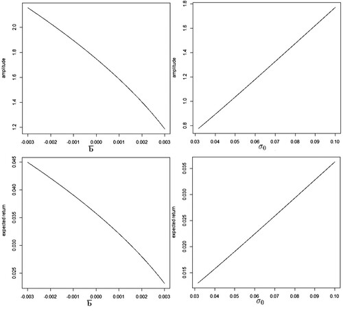
From Tables 9–11, we may observe that the numerical results are consistent with our theoretical analysis. When following the market index it generates the higher expected return and the amplitude is the higher too. On the other hand, since the random target is taken as the market index from the same market, it is reasonable to have positive covariances between the underlying assets and the index. This decreases the target impacts. Then, the amplitude, expected returns and target impact are all lowered due to the positive covariances and smaller variances of the indices. In particular, we can observe negative target impacts in this case. As such, the random targets' impact is summarized by a singe scale $a^{\ast }$, and we can use the portfolio amplitude to characterize the optimal portfolio following random targets. If the amplitude of the optimal portfolio is high, then the investor is not only seeking minimal downside risk but also the higher expected returns, which implies more aggressive trading in his/her portfolio. To further demonstrates the monotonicity, we present Figure 1.

Figure 1. The monotonicity between the expected return, the target impact and the portfolio amplitude.

3.4. Example 4: following random targets when $\mathbf{b}$ is unknown

In this example, we discuss the downside risk optimization following random target from a different market. We consider two cases using the same data of previous examples in the year of 2019. In particular, in the first case we consider weekly returns of the stocks in NYSE market following the NASDAQ index and the 10-year Treasury bond, respectively. Similarly, we consider weekly returns of stocks in Shanghai stock market following the Tokyo stock market index and the 10-year China government bond, respectively. In both cases, it could be insensible to have direct estimation of $\mathbf{b}$ between selected stocks and indices ; however, we may assume that the covariances between the stocks and the market index are positive, i.e. $\mathbf{b}>0$, whilst the covariance between the stocks and the bonds are negative, i.e. $\mathbf{b}<0$ (Singer 2010). Then, using our methodology, we can compute the optimal portfolio when $\mathbf{b}=0$ as a bound to decide whether to follow the random target without estimating the covariances.

From Table 12, we have the optimal portfolio under the downside risk optimization following the random target when $\mathbf{b}$ is taken as 0. Based on our analysis, such portfolio can be regarded as a bound for investors to decide whether to follow the random targets. For instance, it is reasonable to assume $\mathbf{b}>0$ for stock market index, especially for NASDAQ index as the two markets are both in USA. Then, following the market index should generally result in lower target impact and amplitude than the one in the table. Hence, using Proposition 2.14, we may expect the optimal portfolio following the market index would have lower expected return than the expected returns in the table without knowing the estimation of $\mathbf{b}$. If the investor would like to have minimal target shortfall with higher expected return, then he or she should seek other targets rather than the market index provided in this example. Likewise, we assume negative $\mathbf{b}$ between the stocks and the bonds. Then, the optimal portfolios following bonds should have higher expected return than the ones presented in the table. In this regard, our results could explain why investors would construct a stock portfolio following a bond; such investment strategy can have a portfolio that minimizes the target shortfall with respect to the bond and maintains higher expected return simultaneously.

Table 12. Optimal portfolios minimizing the downside risk with random targets when b = 0. Results are based on the data of 2019.

		NASDAQ index	10-year Treasury bond
	target shortfall	0.005891201	0.001051524
NYSE	expected return	0.01629083	0.008246773
	target impact a	0.0003139947	5.792545e−09
	amplitude	1.942691	0.6643609
		Tokyo index	10-year China government bond
	target shortfall	0.005837583	0.002336484
Shanghai	expected return	0.01934497	0.00903813
	target impact a	0.0003279026	2.830799e−10
	amplitude	1.365159	0.7469125

4. Conclusion

Downside risk optimization is an appealing method for portfolio management in both financial and actuarial context. It fits investors' risk averse appetite by minimizing the downside risk and provides flexibility to follow targets based on the investor's preference. In this paper, we derive the explicit solutions to the downside risk optimizations of the first four orders lower partial moments with constant targets. Motivated by the passive portfolio management, we also derive the explicit formulas to the optimal portfolio minimizing the target shortfall with respect to a random target under the multivariate elliptical distributions, and present Gaussian model, Student's t model and symmetric Variance Gamma model as special examples. With some ad hoc assumptions, we analytically prove a mechanism by which the random target influences portfolio selection. In doing so, we propose using portfolio amplitude, as a new measure in the literature, to characterize the impact of following random targets. We present numerical examples based on the data from stock markets across the world to support our theoretical results. In particular, we show that our theoretical analysis could still hold empirically without the ad hoc assumption. Thus, our work in this paper provides new and useful insights into the management of portfolios' downside risk for both financial and actuarial applications. It is our aim to extend the results in this paper to more general models in future research papers.

Acknowledgments

The author wishes to express their indebtedness to the anonymous reviewers and the editor for their many insightful remarks and invaluable comments that helped them improve the paper to a significant extent.

Disclosure statement

No potential conflict of interest was reported by the author(s).

Additional information

Funding

This research was supported by the Israel Science Foundation [grant No. 1686/17) and The Zimmerman Foundation for the study of Banking and Finance. Ming Zhou and Jing Yao also acknowledge National Natural Science Foundation of China [grant no. 11971506). Jing Yao acknowledge London Mathematical Society [grant Ref.42006].

Notes on contributors

Zinoviy Landsman

Zinoviy Landsman Earned his MA in Probability and Statistics in Tashkent State University (1972) and his PhD in Statistics in Romanovsky Mathematical Institute, Department of Mathematical Statistics, Academy of Sciences of Uzbekistan (1978). He is a professor in University of Haifa (from 2007), and he is now the Director of Actuarial Research Center, University of Haifa and a professor of Holon Institute of Technology, Israel.

Udi Makov

Udi Makov has earned his PhD in Mathematical Statistics from University College London and he is currently a Professor of Statistics at the University of Haifa, Israel.

Jing Yao

Jing Yao obtained his PhD in Economics from Vrije Universiteit Brussel in 2013. He is currently associate professor at Maxwell Institute for Mathematical Science and Heriot-Watt University.

Ming Zhou

Ming Zhou earned his PhD at Nankai University (2006) and did Post-Doctoral Fellow at University of Waterloo (2007). Now he is a Professor in Risk Management and Actuarial Science at Renmin University of China and he is also an Associate (ASA) of Society of Actuaries.

Notes

1 In fact, to completely replicate a market index is possible but costly. A market index often consists of a considerable number of traded assets in the market. Full replication would result in over loaned transaction cost. Moreover, the assets that constitute the market index are not always the same and frequent adaptation is inevitable. Therefore, full replication could be averse for passive portfolio management and many index funds are constructed based on a few selected traded assets (Beasley, Meade, and Chang 2003).

2 By contrast, the so-called ‘active’ portfolio management of index tracking is aimed at outperforming the index with frequent trading; see, e.g. Elton, Gruber, and Blake (1995).

3 There is other research strands that study how to invest in the market directly; see for instance (Basak, Shapiro, and Teplá 2006).

4 It is usual that one has an additional constraint on the expected return of the portfolio in downside risk optimization, i.e. $\underset{\mathbf{w}}{min}E[({\mathbf{w}}^T\mathbf{X}-X_0{)}^{-}]\mathrm{subject}\mathrm{to}{\mathbf{1}}^T\mathbf{w}=1\mathrm{and}{\mathbf{w}}^T\mu =c,$where $\mu$ is the expected returns of $\mathbf{X}$ and c is the constant. However, in the context of normal distribution, such optimization has the same optimal solution with the minimization of portfolio variance and has been well-documented in the literature (cf. Corollary 4, Klebaner et al. (2017)). Hence, we focus on (3(3) $\underset{\mathbf{w}}{min}E[(({\mathbf{w}}^T\mathbf{X}-X_0{)}^{-})]\mathrm{subject}\mathrm{to}{\mathbf{1}}^T\mathbf{w}\mathbf{=}1.$(3) ) in our paper.

5 Note that to ensure that the covariance matrix is positive definite, the components in $\mu$ cannot be identical, i.e. $\mu \ne c\mathbf{1}$, where c is a constant.

6 In general, an elliptical distribution does not necessarily has the density function. We focus on the case where the density function exists in this paper.

Appendix

Proof to Theorem 2.1.

For i = 1, 2, the proofs can be found in Klebaner et al. (2017). We prove $i=3$ as follows. First note that (A1) $\frac{\mathrm{\partial }E[((X-K{)}^{-}{)}^3]}{\mathrm{\partial }\sigma }=6\sigma ((K-\mu )\mathrm{\Phi }\left(\frac{K-\mu }{\sigma }\right)+\sigma \phi \left(\frac{K-\mu }{\sigma }\right)),$(A1) and the equation inside the bracket of the right-hand-side is $E[((X-K{)}^{-})]>0$; thus (A1(A1) $\frac{\mathrm{\partial }E[((X-K{)}^{-}{)}^3]}{\mathrm{\partial }\sigma }=6\sigma ((K-\mu )\mathrm{\Phi }\left(\frac{K-\mu }{\sigma }\right)+\sigma \phi \left(\frac{K-\mu }{\sigma }\right)),$(A1) ) is increasing at σ. Thus, for a given expected return z, downside risk optimization (2(2) $\underset{\mathbf{w}}{min}E[(({\mathbf{w}}^T\mathbf{X}-K{)}^{-}{)}^i]\mathrm{subject}\mathrm{to}{\mathbf{1}}^T\mathbf{w}\mathbf{=}1,$(2) ) is equivalent to minimizing ${\mathbf{w}}^T\mathbf{\Sigma }\mathbf{w}$ subject to ${\mathbf{w}}^{\mathbf{T}}\mu =z$ and ${\mathbf{w}}^{\mathbf{T}}\mathbf{1}=1$, and the explicit solution is (Landsman 2008) $\mathbf{w}={\mathbf{\Sigma }}^{-1}{A}_K^T(A_K{\mathbf{\Sigma }}^{-1}{A}_K^T{)}^{-1}\mathbf{z},$We then need is find the optimal $z_0$ that determines the optimal weight. To this end, take ${\mathbf{w}}^{\mathbf{T}}(\mu -K\mathbf{1})=z_0-K=z$. Then, the objective function is $h(z)=-(z^3+zq(z))\mathrm{\Phi }\left(\frac{-z}{\sqrt{q(z)}}\right)+(\sqrt{q(z)}{z}^2+2(\sqrt{q(z)}{)}^3)\phi \left(\frac{-z}{\sqrt{q(z)}}\right).$With some tedious calculation, we can show that $h(z)$ is a convex function and has a global minimum at the solution of $h^{\mathrm{\prime }}(z)=0$. The proof for i = 4 is similar, and we omit it here.

Proof to Theorem 2.2.

By accommodating the notations in (4(4) $(\mathbf{X},X_0{)}^T\sim N_{n+1}((\mathit{\mu }\mathbf{,}{\mu }_0{\mathbf{)}}^T,\left(\begin{array}{cc}\mathbf{\Sigma }& \mathbf{b}\\ {\mathbf{b}}^T& {\sigma }_0^2\end{array}\right)),$(4) ) to Theorem 2.1, we can see Theorem 2.2 follows directly.

Proof to Theorem 2.5.

First note that, for a univariate elliptical random variable $X\sim E_1(\mu ,\sigma ,g_1)$, $E[(X-K{)}^{-}]=\sigma {\int }_{-\mathrm{\infty }}^{\frac{K-\mu }{\sigma }}(\frac{K-\mu }{\sigma }-x)f(x)\mathrm{d}x,$where $f(x)$ is the density function of X's standard form, i.e. $X\sim E_1(0,1,g_1)$, and $f(x)=g_1(\frac{x^2}{2})$. Denoting X's associate as $X^{\ast }$ and using the connection between X and $X^{\ast }$, i.e. $(f^{\ast }(x){)}^{\mathrm{\prime }}=-xf(x)$, we have $\begin{array}{rl}E[(X-K{)}^{-}]& =(K-\mu )F\left(\frac{K-\mu }{\sigma }\right)+\sigma {\int }_{-\mathrm{\infty }}^{\frac{K-\mu }{\sigma }}(f^{\ast }(x){)}^{\mathrm{\prime }}\mathrm{d}x.\\ & =(K-\mu )F\left(\frac{K-\mu }{\sigma }\right)+\sigma f^{\ast }\left(\frac{K-\mu }{\sigma }\right).\end{array}$It is then easy to verify that $\frac{\mathrm{\partial }E[(X-K{)}^{-}]}{\mathrm{\partial }\sigma }>0$, i.e. $E[(X-K{)}^{-}]$ is an increasing function of σ for given μ and K. Thus, similarly with Theorem 2.1, minimising the expected shortfall for given expected return and fixed target has the same solution to minimising the variance for given expected return, and we need to show $h(c)=-cF\left(\frac{-c}{\sqrt{q(z)}}\right)+\sqrt{q(z)}{f}^{\ast }\left(\frac{-c}{\sqrt{q(z)}}\right)$is a convex function of c. With some calculation, we can show that $h^{\mathrm{\prime }\mathrm{\prime }}(c)=f^{\ast }\left(\frac{-c}{\sqrt{q(z)}}\right)\frac{q_1{q}_3-q_2^2}{(\sqrt{q(z)}{)}^3}+f\left(\frac{-c}{\sqrt{q(z)}}\right)\frac{(q_{2}c-q_3{)}^2}{(\sqrt{q(z)}{)}^5},$which justify that $h(c)$ is convex and has unique minimum at $h^{\mathrm{\prime }}(c)=0$. Therefore, we have the theorem holds.

Density function of multivariate Student's t distribution and symmetric Variance Gamma distribution

Student's t distribution:

For ${\mathbf{X}}^T\sim t_n(\nu ,{\mu }^T,\frac{\nu }{\nu -2}\mathbf{\Sigma })$, the density function is $f(\mathbf{x})=\frac{\mathrm{\Gamma }\left(\frac{\nu +n}{2}\right)}{(\sqrt{\nu \pi }{)}^n\mathrm{\Gamma }\left(\frac{\nu }{2}\right)}{(1+\frac{(\mathbf{x}-\mu {)}^T{\mathbf{\Sigma }}^{-1}(\mathbf{x}-\mu )}{\nu })}^{-\frac{\nu +n}{2}}$In particular, for $X\sim t(\nu ,0,\frac{\nu }{\nu -2}),$ the density function is $f(x)=\frac{\mathrm{\Gamma }(\frac{\nu +1}{2})}{\sqrt{\nu \pi }\mathrm{\Gamma }(\frac{\nu }{2})}(1+\frac{x^2}{\nu }{)}^{-\frac{\nu +1}{2}}$

Symmetric Variance Gamma:

For ${\mathbf{X}}^T\sim SV{G}_n(\lambda ,{\mu }^T,\lambda \mathbf{\Sigma })$, the density function is $f(\mathbf{x})=\frac{2^{-\lambda +1+\frac{d}{2}}}{{\left(2\pi \right)}^{\frac{d}{2}}{\left|\mathbf{\Sigma }\right|}^{\frac{1}{2}}\mathrm{\Gamma }(\lambda )}\frac{K_{\lambda -\frac{d}{2}}(\sqrt{2(\mathbf{x}-\mu {)}^T{\mathbf{\Sigma }}^{-1}(\mathbf{x}-\mu )})}{(\sqrt{2(\mathbf{x}-\mu {)}^T{\mathbf{\Sigma }}^{-1}(\mathbf{x}-\mu )}{)}^{-\lambda +\frac{d}{2}}}$In particular, for $X\sim SVG(\lambda ,0,\lambda ),$ the density function is $f(x)=\frac{2^{-\lambda +\frac{3}{2}}{K}_{\lambda -\frac{1}{2}}(\sqrt{2x^2})}{\sqrt{2\pi }\mathrm{\Gamma }(\lambda )(\sqrt{2x^2}{)}^{-\lambda +\frac{1}{2}}}.$

The following Lemma can be easily proved by taking derivatives of the associated functions.

Lemma A.1

The following two statements are true.

1. $\phi (-t)\frac{1}{t}-\mathrm{\Phi }(-t)$ is a non-increasing and positive function of t for t>0.

2. $\phi (t)t-\mathrm{\Phi }(t)$ is a decreasing and negative function of t for t>0.

Proof to Proposition 2.9.

Due to positive-definite matrices, it holds that $p_1>0$, $p_3>0$ and $p_1{p}_3-p_2^2>0$. Define the equation in (5(5) $\phi \left(\frac{-z}{\sqrt{p(z)}}\right)(p_{1}z-p_2)=\sqrt{p(z)}\mathrm{\Phi }\left(\frac{-z}{\sqrt{p(z)}}\right).$(5) ) as $g(z):=$ $\phi (\frac{-z}{\sqrt{q(z)}})(p_{1}z-p_2)-\sqrt{q(z)}\mathrm{\Phi }(\frac{-z}{\sqrt{q(z)}})=0$. It is straightforward to see $g(z)$ is an increasing function based on Theorem 2.2.

For (9(9) $\begin{array}{rl}{p}_1{z}_1-p_2& >0;\end{array}$(9) ), note that $g(z_1)=0$ and $g(\frac{p_2}{p_1})<0$ always hold. Due to the monotonicity of g, we have that (9(9) $\begin{array}{rl}{p}_1{z}_1-p_2& >0;\end{array}$(9) ) is true.

For (10(10) $\begin{array}{rl}{p}_2{z}_1-p_3& <0.\end{array}$(10) ), if $p_2>0$, following Lemma A.1, we have $g\left(\frac{p_3}{p_2}\right)=\phi (-\sqrt{\frac{p_3}{p_1{p}_3-p_2^2}})\left(\sqrt{\frac{p_1{p}_3-p_2^2}{p_3}}\right)-\mathrm{\Phi }(-\sqrt{\frac{p_3}{p_1{p}_3-p_2^2}})>0.$Hence, $z_1<\frac{p_3}{p_2}$. If $p_2<0,$ $\frac{p_2}{p_1}-\frac{p_3}{p_2}=\frac{p_2^2-p_1{p}_3}{p_1{p}_2}>0;$thus, again, $z_1>\frac{p_2}{p_1}>\frac{p_3}{p_2}$, which concludes the proof.

Proof to Theorem 2.11.

We first show that $z_1$ is increasing with respect to $p_3$ in model (4(4) $(\mathbf{X},X_0{)}^T\sim N_{n+1}((\mathit{\mu }\mathbf{,}{\mu }_0{\mathbf{)}}^T,\left(\begin{array}{cc}\mathbf{\Sigma }& \mathbf{b}\\ {\mathbf{b}}^T& {\sigma }_0^2\end{array}\right)),$(4) ).

Note that $z_1$ is an implicit function of $p_3$ according to Equation (5(5) $\phi \left(\frac{-z}{\sqrt{p(z)}}\right)(p_{1}z-p_2)=\sqrt{p(z)}\mathrm{\Phi }\left(\frac{-z}{\sqrt{p(z)}}\right).$(5) ), for which $\frac{\mathrm{\partial }{z}_1}{\mathrm{\partial }{p}_3}=-\frac{\mathrm{\partial }g}{\mathrm{\partial }{p}_3}/\frac{\mathrm{\partial }g}{\mathrm{\partial }{z}_1}.$Theorem 2.2 indicates that $\frac{\mathrm{\partial }g}{\mathrm{\partial }{z}_1}>0$. Thus, we only need to show that $\frac{\mathrm{\partial }f}{\mathrm{\partial }{p}_3}<0.$ We compute $\begin{array}{rl}\frac{\mathrm{\partial }g}{\mathrm{\partial }{p}_3}& =-\phi \left(\frac{-z_1}{\sqrt{q(z_1)}}\right)\ast \frac{H(z_1)}{2(\sqrt{q(z_1)}{)}^5},\\ H(z_1)& =(p_1{z}_1-p_2)q(z_1)+z_1(p_3-p_2{z}_1).\end{array}$We can see that $H(z_1)>0$ holds because of Proposition 2.9.

Moreover, under the assumption that $\mathbf{b}=b\mathbf{1}$, we have $q_3=a+s^{-1}{u}_3$, for which $z_1$ is increasing with respect to a.

Proof to Theorem 2.13.

Note that $\begin{array}{rl}{\mathbf{\Sigma }}_{\mathbf{Y}}^{-1}& ={\mathbf{\Sigma }}^{-1}-\frac{a{\mathbf{\Sigma }}^{-1}{\mathbf{1}{\mathbf{1}}^{\mathbf{T}}\mathbf{\Sigma }}^{-1}}{1+a{u}_1},\\ {\mathbf{\Sigma }}_{\mathbf{Y}}^{-1}{A}_{\mathbf{Y}}^T& =(\frac{{\mathbf{\Sigma }}^{-1}\mathbf{1}}{1+a{u}_1},{\mathbf{\Sigma }}^{-1}{\mu }_{\mathbf{Y}}-\frac{a{\mathbf{\Sigma }}^{-1}\mathbf{1}{u}_2}{1+a{u}_1}).\end{array}$With Theorem 2.2, we can rewrite the optimal weights as (A2) $\begin{array}{rl}{\mathbf{w}}_1& ={\mathbf{\Sigma }}_{\mathbf{Y}}^{-1}{A}_{\mathbf{Y}}^T(A_{\mathbf{Y}}{\mathbf{\Sigma }}_{\mathbf{Y}}^{-1}{A}_{\mathbf{Y}}^T{)}^{-1}{\mathbf{z}}_1\\ & =s^{-1}({\mathbf{\Sigma }}^{-1}\mathbf{1}\mathbf{(}{u}_3-u_2{z}_1\mathbf{)}\mathbf{)}\mathbf{+}{\mathbf{\Sigma }}^{\mathbf{-}\mathbf{1}}{\mu }_{\mathbf{Y}}\mathbf{(}{u}_1{z}_1-u_2\mathbf{)}\mathbf{)}\\ & =s^{-1}(\mathbf{u}+z_1\mathbf{v})\end{array}$(A2) where $\begin{array}{rl}\mathbf{u}& =u_3{\mathbf{\Sigma }}^{-1}\mathbf{1}-u_2{\mathbf{\Sigma }}^{\mathbf{-}\mathbf{1}}{\mu }_{\mathbf{Y}}\\ \mathbf{v}& =u_1{\mathbf{\Sigma }}^{\mathbf{-}\mathbf{1}}{\mu }_{\mathbf{Y}}-u_2{\mathbf{\Sigma }}^{-1}\mathbf{1.}\end{array}$Let us assume that $max({\mathbf{w}}_1)={\mathbf{w}}_1[I]$ and $min({\mathbf{w}}_1)={\mathbf{w}}_1[J]$ for some $I,J\in \{1,2,\dots ,n\}$. Then, $\begin{array}{rl}Amp({\mathbf{w}}_1)& ={\mathbf{w}}_1[I]-{\mathbf{w}}_1[J]\\ & =s^{-1}((\mathbf{v}[I]-\mathbf{v}[J])z_1+(\mathbf{u}[I]-\mathbf{u}[J]).\end{array}$We are able to conclude that $\mathbf{v}[I]-\mathbf{v}[J]>0$ because otherwise $Amp({\mathbf{w}}_1)$ would go negative for large $z_1,$ which cannot be the case. Hence, $Amp({\mathbf{w}}_1)$ is increasing with respect to $z_1$.

References

- Basak, S., A. Shapiro, and L. Teplá. 2006. “Risk Management with Benchmarking.” Management Science 52 (4): 542–557.
- Beasley, J. E., N. Meade, and T. J. Chang. 2003. “An Evolutionary Heuristic for the Index Tracking Problem.” European Journal of Operational Research 148 (3): 621–643.
- Cumova, D., and D. Nawrocki. 2014. “Portfolio Optimization in An Upside Potential and Downside Risk Framework.” Journal of Economics and Business 71: 68–89.
- De Franco, C., and P Tankov. 2011. “Portfolio Insurance Under a Risk-Measure Constraint.” Insurance: Mathematics and Economics 49 (3): 361–370.
- DeMiguel, V., L. Garlappi, and R. Uppal. 2009. “Optimal Versus Naive Diversification: How Inefficient is the 1/N Portfolio Strategy?” The Review of Financial Studies 22 (5): 1915–1953.
- Elton, E. J., M. J. Gruber, and C. R Blake. 1995. “Fundamental Economic Variables, Expected Returns, and Bond Fund Performance.” The Journal of Finance 50 (4): 1229–1256.
- French, K. R., and J. M. Poterba. 1991. “Investor Diversification and International Equity Markets (No. w3609).” National Bureau of Economic Research.
- Gharakhani, M., F. Zarea Fazlelahi, and S. J. Sadjadi. 2014. “A Robust Optimization Approach for Index Tracking Problem.” Journal of Computer Science 10 (12): 2450–2463.
- Haberman, S., and E. Vigna. 2002. “Optimal Investment Strategies and Risk Measures in Defined Contribution Pension Schemes.” Insurance: Mathematics and Economics 31 (1): 35–69.
- Harlow, W. V. 1991. “Asset Allocation in a Downside-Risk Framework.” Financial Analysts Journal 47 (5): 28–40.
- Harlow, W. V., and R. K. S. Rao. 1989. “Asset Pricing in a Generalize Mean-Lower Partial Moments Framework: Theory and Evidence.” Journal of Financial and Quantitative Analysis 24: 285–309.
- Klebaner, F., Z. Landsman, U. Makov, and J. Yao. 2017. “Optimal Portfolios with Downside Risk.” Quantitative Finance 17 (3): 315–325.
- Landsman, Z. 2008. “Minimization of the Root of a Quadratic Functional Under a System of Affine Equality Constraints with Application to Portfolio Management.” Journal of Computational and Applied Mathematics 220 (1-2): 739–748.
- Landsman, Z., and J. Nešlehová. 2008. “Stein's Lemma for Elliptical Random Vectors.” Journal of Multivariate Analysis 99 (5): 912–927.
- Landsman, Z., S. Vanduffel, and J. Yao. 2013. “A Note on Stein's Lemma for Multivariate Elliptical Distributions.” Journal of Statistical Planning and Inference 143 (11): 2016–2022.
- Landsman, Z., S. Vanduffel, and J. Yao. 2015. “Some Stein-Type Inequalities for Multivariate Elliptical Distributions and Applications.” Statistics & Probability Letters 97: 54–62.
- Ling, A., J. Sun, and X. Yang. 2014. “Robust Tracking Error Portfolio Selection with Worst-Case Downside Risk Measures.” Journal of Economic Dynamics and Control 39: 178–207.
- Malkiel, B. G., and E. F. Fama. 1970. “Efficient Capital Markets: A Review of Theory and Empirical Work.” The Journal of Finance 25 (2): 383–417.
- Markowitz, H. M. 1987. Mean-Variance Analysis in Portfolio Choice and Capital Markets. Oxford: Blackwell.
- Platanakis, E., and C. Sutcliffe. 2016. “Pension Scheme Redesign and Wealth Redistribution Between the Members and Sponsor: The USS Rule Change in October 2011.” Insurance: Mathematics and Economics69: 14–28.
- Platanakis, E., and C. Sutcliffe. 2017. “Asset–Liability Modelling and Pension Schemes: The Application of Robust Optimization to USS.” The European Journal of Finance 23 (4): 324–352.
- Platanakis, E., C. Sutcliffe, and A. Urquhart. 2018. “Optimal Vs Naïve Diversification in Cryptocurrencies.” Economics Letters 171: 93–96.
- Platanakis, E., C. Sutcliffe, and X. Ye. 2021. “Horses for Courses: Mean-Variance for Asset Allocation and 1/N for Stock Selection.” European Journal of Operational Research 288 (1): 302–317.
- Platanakis, E., and A. Urquhart. 2019. “Portfolio Management with Cryptocurrencies: The Role of Estimation Risk.” Economics Letters 177: 76–80.
- Platanakis, E., and A. Urquhart. 2020. “Should Investors Include Bitcoin in Their Portfolios? A Portfolio Theory Approach.” The British Accounting Review 52 (4): 100837.
- Roman, D., G. Mitra, and V. Zverovich. 2013. “Enhanced Indexation Based on Second-Order Stochastic Dominance.” European Journal of Operational Research 228 (1): 273–281.
- Rudolf, M., H. J. Wolter, and H. Zimmermann. 1999. “A Linear Model for Tracking Error Minimization.” Journal of Banking & Finance 23 (1): 85–103.
- Singer, N. 2010. “Safety-First Portfolio Optimization: Fixed Versus Random Target (No. 113).” Thüen-Series of Applied Economic Theory-Working Paper.
- Zhu, S., D. Li, and S. Wang. 2009. “Robust Portfolio Selection Under Downside Risk Measures.” Quantitative Finance 9 (7): 869–885.