Hedge fund return predictability in the presence of model risk*

ABSTRACT

Hedge funds implement elaborate investment strategies that include a variety of positions and assets. As a result, there is significant time variation in the set of risk factors and their respective loadings which in turn introduces severe model risk in any attempt to model and forecast hedge fund returns. In this study, we investigate the statistical and economic value of incorporating heteroscedasticity, non-normality, time-varying parameters, model selection risk and parameter estimation risk jointly in hedge fund return forecasting and fund of funds construction. Parameter estimation risk is dealt with a time-varying parameter structure, while model selection uncertainty is mitigated by model averaging or model selection. We adopt a dynamic model averaging approach along with the conventional Bayesian averaging technique. Our empirical results suggest that accounting for model risk can significantly improve the forecasting accuracy of hedge fund returns and consequently the performance of funds of hedge funds.

KEYWORDS:

• Forecasting
• Hedge funds
• dynamic model averaging
• model risk
• fund of funds

1. Introduction

Hedge funds constitute lightly regulated vechicles that promise enchanced performance in all market conditions. To do so, hedge funds employ various sophisticated investment strategies that lead to option-like payoffs and infuse their return distribution with characteristics that differentiate them from traditional asset classes, such as bonds and stocks. Therefore, identifying ways that improve hedge fund return predictability is crucial for optimally defining an investment strategy in hedge funds. To this end, a long list of linear and non-linear risk factors have been proposed, including the Fung and Hsieh asset-based factors, the three Fama-French factors and Carhart's momentum factor, amongst various macroeconomic and financial variables.¹

Predicting hedge funds returns stumbles into obstacles associated with various aspects of model risk. First, there is uncertainty regarding the appropriate set of predictors. This inability of identifying the most appropriate set of factors, or else ‘model uncertainty’, is well established in the traditional asset pricing literature. However, for the hedge funds asset class ‘model uncertainty’ is aggravated by the unique characteristics of their strategies, which call for additional constraints in defining the appropriate set of factors. S. D. Vrontos, Vrontos, and Giamouridis (2008) highlight the magnitude of model uncertainty finding that the posterior probabilities of the ten most probable linear specifications sum to only 18%. Second, hedge fund managers dynamically rebalance their portfolios, thus infusing each factor loading with time-variation, a feature commonly referred to as ‘parameter estimation risk’. Therefore, as stressed by Fung and Hsieh (2004), Fung et al. (2008), Eling and Faust (2010) and Wegener, von Nitzsch, and Cengiz (2010), the parameter estimates and the set of relevant risk factors may change over time. Third, empirical evidence suggests that, due to their characteristics, hedge fund returns exhibit heteroscedasticity, non-normality and fat tails.

To address various sources of model risk, S. D. Vrontos, Vrontos, and Giamouridis (2008) show that a Bayesian Model Averaging approach that accounts for heteroscedasticity improves the pricing of the managers' skills. Similarly, Wegener, von Nitzsch, and Cengiz (2010) employ a specification that recursively excludes the extraneous factors to account for model uncertainty and they use a rolling estimate scheme to account for time variation in parameter estimates. Their results suggest that a non-parametric regression delivers significant gains in returns predictability. From a different perspective, Slavutskaya (2013) employs a panel data approach to overcome the effect of small samples in the estimation process. The author finds an improved out-of-sample accuracy of factor models. Focusing on aggregate data (hedge fund indices), Panopoulou and Vrontos (2015) build on the results of Avramov, Barras, and Kosowski (2013) who find that combining information from single predictor strategies leads to superior selection ability in the presence of inaccurate individual forecasts. Specifically, Panopoulou and Vrontos (2015) account for various model risk sources by implementing a large number of information and forecast combination strategies to unveil significant gains in forecasts accuracy and economic value. Following the respective literature, our paper holds the middle ground between S. D. Vrontos, Vrontos, and Giamouridis (2008) and Panopoulou and Vrontos (2015) as we combine time-varying coefficient models with model averaging/selection schemes and heteroscedastic variance, to account simultaneously for various sources of model risk.

To account for changes in hedge fund strategies, we adopt a time-varying parameter (TVP) model setting with the parameter estimation error assessed by calibrating the posterior distributions of the parameters. Furthermore, to combine or select the most relevant specifications from a set of popular predictors, we utilize the Dynamic Model Averaging (DMA) and Dynamic Model Selection (DMS) methodologies introduced by Koop and Korobilis (2012) in inflation forecasting.² Contrary to the simple Bayesian Model Averaging (BMA) methods, the DMA techniques dynamically update the model probability at the end of each period rather than applying a constant model probability.³ In other words, instead of selecting the appropriate factors, weights are assigned to filtered information (individual forecasts) that arise from the most probable specifications. This approach is in line with the results of Wegener, von Nitzsch, and Cengiz (2010) and Panopoulou and Vrontos (2015), who suggest that reselecting the factors at regular time intervals and combining individual forecasts, respectively, improves accuracy. Another benefit of this approach is that the information update process does not rely on a Markov Chain Monte Carlo (MCMC) algorithm. Therefore, there is a significant decrease in computational time. For all competing specifications, we model the heteroscedasticity of returns via an exponentially weighted moving average (EWMA) approach, to avoid introducing additional estimation risk in our forecasts. Finally, while we do not account directly for the non-normality and excessive kurtosis of returns, any resulting impact on the estimation process is partially treated by the EWMA specification and the non-linear risk factors advocated by Fung and Hsieh (2004) and Agarwal and Naik (2004). To the best of our knowledge, this is the first time that a study addresses all the above issues jointly.

To evaluate the accuracy of our point forecasts, we first forecast the returns of aggregate hedge fund indices and compare the out-of-sample Mean Square Forecasting Error (MSFE) of each competing specification with the MSFE of a simple benchmark autoregressive OLS-AR(1) model. Since gains in point forecast accuracy do not always translate in additional economic value, we assume the position of a risk-averse investor and use utility-based measures to evaluate the economic significance of the gains in forecasting accuracy. In this set-up, the economic evaluation exercise is tantamount to evaluating the predictive density as a whole and not just the point forecasts. Furthermore, we evaluate the performance of our proposed methodology on individual funds by creating hypothetical funds of funds. Our fund selection approach is in line with Agarwal, Green, and Ren (2018), as we focus on the return forecasts instead of chasing past performance in the form of alpha.

As our first contribution, we explore whether our proposed methodology improves the accuracy of point forecasts of hedge fund returns. Our findings suggest that, in terms of point forecast accuracy, simple TVP-AR(1) specifications coupled with heteroscedastic variances can adequately provide significant forecasting improvements. However, when we account for the size of the underlying funds, the BMA, BMS and DMA methods exhibit superior forecasting performance. The negative size-return relationship is well documented in the hedge fund literature. For example, Joenvaara, Kosowski, and Tolonen (2019), Yin and Zhang (2019) and Gao, Haight, and Yin (2019) find that smaller funds yield larger returns. Our findings suggest that the BMA, BMS and DMA models' performance are superior to the TVP-AR(1), once the size-effect is accounted for. Our value weighted indices are more homogeneous compared to the equally weighted ones and driven by a few large size funds. As such, they are more exposed to market factors captured by our predictor list rendering the BMA, BMS and DMA models superior to the simple TVP-AR(1) that does not include any predictors.

Our second contribution builds on the results of the statistical evaluation and investigates whether the forecasting accuracy gains are translated to economic gains. Under the prism of a risk-averse investor, we find that our proposed methods deliver a significantly larger Certainty Equivalent Return (CER) than the benchmark. Our economic evaluation results corroborate the statistical evidence and point towards the superior performance of the TVP specifications coupled with persistent volatility specifications.

Finally, our third contribution emerges from our fund of funds portfolio performance results. Specifically, we find that constructing portfolios based on methods that account for model risk is a superior approach relative to the benchmark. However, these specifications are sensitive to the investor's strategy and the weighting scheme adopted. When we focus on chasing returns, the TVP-AR(1) and DMA methods deliver the best performing portfolios. When we select funds according to the accuracy of forecasts, model averaging/selection methods under mean-variance and mean-CVaR optimization appear superior. Moreover, the crisis evaluation sample highlights the importance of such methods as, depending on the weighting schemes, the TVP and DMA methods select the best performing portfolios.

The rest of the paper is organized as follows: Section 2 describes the forecasting methodologies used in the paper, Section 3 describes the data, and Section 4 presents the empirical results and the predictive ability of the proposed methods. Section 5 presents the portfolio formation strategy and the related findings, while Section 6 concludes.

2. Return prediction models

2.1. Time-varying parameter model

Under the Bayesian framework, the Kalman Filter provides a simple way to recursively forecast the unobservable states (i.e. the coefficients of prediction factors in linear regression models), given new data observations. The normal linear state-space model can be described schematically as a linear regression model with time-varying parameters (Meinhold and Singpurwalla 1983; Koop and Korobilis 2012). Specifically, the normal linear state-space model is defined as: (1) $\begin{array}{rl}{r}_t& =X_{t-1}{\beta }_t+{\epsilon }_t\\ {\beta }_t& ={\beta }_{t-1}+{\eta }_t\end{array}$(1) where $r_t$ is the hedge fund return at time t, ${\mathbf{X}}_{t-1}$ is the vector of predictors with the first column being 1, ${\beta }_t$ is the vector of coefficients, ${\epsilon }_t$ is the regression residual of hedge fund returns (with ${\epsilon }_t\sim N(0,H_t)$), and ${\eta }_t$ is the residual of predictive coefficients (with ${\eta }_t\sim N(0,Q_t)$). The two error terms are assumed to be independent from each other. Equivalently, the above state-space model can be interpreted as a linear hedge fund returns predictive model with time-varying risk exposures ${\beta }_t$. Contrary to the constant coefficient models, time-varying parameter (TVP) models accommodate the variation of coefficients, by allowing them to vary as new observations are added to the data.

The ordinary Kalman filter begins with the posterior result of parameters that satisfies the following: (2) ${\beta }_{t-1}\mid r^{t-1}\sim N({\hat{\beta }}_{t-1},{\mathrm{\Sigma }}_{t-1\mid t-1})$(2) where $r^{t-1}$ denotes the information set of hedge fund returns from time 0 to time $t-1$. Then it proceeds to the following predictive step (3) $\begin{array}{rl}{\beta }_t\mid r^{t-1}& \sim N({\hat{\beta }}_{t-1},{\mathrm{\Sigma }}_{t\mid t-1})\\ {\mathrm{\Sigma }}_{t\mid t-1}& ={\mathrm{\Sigma }}_{t-1\mid t-1}+Q_t\end{array}$(3) To simplify the estimation of ${\mathrm{\Sigma }}_{t\mid t-1}$, Raftery, Karny, and Ettler (2010) adopt the following approximation (4) ${\mathrm{\Sigma }}_{t\mid t-1}=\frac{1}{\lambda }{\mathrm{\Sigma }}_{t-1\mid t-1}$(4) where λ acts as a forgetting factor and it is fixed to a number slightly below one ($0<\lambda ⩽1$), so that the coefficients change gradually. Following the model specification, observations that are located m periods in the past would be weighted by ${\lambda }^m$. Raftery, Karny, and Ettler (2010) and Koop and Korobilis (2012) set the forgetting factor to $\lambda =0.99$ and $\lambda =0.95$ for quarterly data. In the case of $\lambda =0.99$, coefficients evolve relatively slowly, while setting $\lambda =0.95$ results in coefficients that are more unstable. For example, when $\lambda =0.99$, the data located at 5 years before time t will receive a weight equal to 80% of the weight assigned to the observation at t−1. However, when $\lambda =0.95$, the respective weight for the observations 5 years ago will be equal to approximately 35% of the weight for the last period observation. To allow for a similar speed of parameter evolution in our monthly dataset we set $\lambda =0.996$ for a gradual change to coefficients and $\lambda =0.985$ for a more abrupt pattern. In essence, employing the forgetting factors is similar to applying a rolling window regression with a window size of $1/(1-\lambda )$, which would roughly correspond to rolling window estimations of 20 and 5 years, respectively. The attractive feature of forgetting factors in this context is that they allow controlling the degree of instability in the coefficients. This is important since it is unclear whether rapidly changing coefficients are useful in forecasting as changing coefficients might inflate estimation errors.⁴

The important advantage of the simplification in Equation (4(4) ${\mathrm{\Sigma }}_{t\mid t-1}=\frac{1}{\lambda }{\mathrm{\Sigma }}_{t-1\mid t-1}$(4) ) is that it eliminates the need to estimate or simulate $Q_t$. When new data arrives, we proceed to the updating step of the Kalman filter ${\beta }_t\mid r^t\sim N({\hat{\beta }}_{t\mid t},{\mathrm{\Sigma }}_{t\mid t})$ where (5) $\begin{array}{rl}& {\hat{\beta }}_{t\mid t}={\hat{\beta }}_{t\mid t-1}+{\mathrm{\Sigma }}_{t\mid t-1}{X}_{t-1}^{\prime }(H_t+X_{t-1}{\mathrm{\Sigma }}_{t\mid t-1}{X}_{t-1}^{\prime }{)}^{-1}(r_t-{\hat{\beta }}_{t\mid t-1}{X}_{t-1})\\ & {\mathrm{\Sigma }}_{t\mid t}={\mathrm{\Sigma }}_{t\mid t-1}-{\mathrm{\Sigma }}_{t\mid t-1}{X}_{t-1}^{\prime }(H_t+X_{t-1}{\mathrm{\Sigma }}_{t\mid t-1}{X}_{t-1}^{\prime }{)}^{-1}{X}_{t-1}{\mathrm{\Sigma }}_{t\mid t-1}\end{array}$(5) In such a set-up, the predictive distribution of returns is given by (6) $r_t\mid r^{t-1}\sim N({\hat{\beta }}_{t-1}{X}_{t-1},H_t+X_{t-1}{\mathrm{\Sigma }}_{t\mid t-1}{X}_{t-1}^{\prime })$(6) Therefore, results are analytical, conditional on $H_t$, and no MCMC algorithm is required to derive the posterior distribution of parameters and the predictive distribution of hedge fund returns. Hence, there is a significant reduction in computational time. Following Koop and Korobilis (2012), we adopt the Exponentially Weighted Moving Average (EWMA) estimator of $H_t$: (7) ${\hat{H}}_t=\sqrt{(1-\kappa )\sum _{j=1}^t{\kappa }^{j-1}(r_j-{\hat{\theta }}_j{X}_j)}$(7) The above specification suggests that the $H_t$ forecast, given the information available up to time $t-1$, has the following analytical form: (8) ${\hat{H}}_{t\mid t-1}=\kappa {\hat{H}}_{t-1\mid t-2}+(1-\kappa )(r_{t-1}-X_{t-1}{\hat{\beta }}_{t-1})$(8) where $\kappa \in [0,1]$ is the decay factor of the EWMA estimator, which plays a similar role to the forgetting factor λ. We adopt two different values for κ at 0.97 and 0.92, in order to allow for different speeds of decay. The chosen values for the decay factor are guided by RISKMETRICS (1996) who provide an analysis for the specific values and the properties of EWMA estimators in general. Riskmetrics recommend a value of 0.97 for monthly data and 0.94 for daily data. For $\kappa =0.97$, the estimation window roughly corresponds to 150 days (5 months) at a 1% tolerance level, while for the quick decay factor ($\kappa =0.92$), the respective window is 56 days (2 months). Volatility forecasts based on more historical observations (slow decay factor) are smoother than those that rely on fewer data points (fast decay factors). Given that hedge fund returns are quite volatile and exhibit a high degree of heteroscedasticity Giamouridis and Vrontos (2007), we also consider the fast decay factor.

Given all the specifications, the system can be estimated with initial conditions for ${\theta }_0$ and $H_0$.⁵ One important drawback of the TVP model is that the set of predictors remains unchanged throughout time. As a hedge fund manager dynamically adjusts the fund's composition, allowing for time variation of coefficients on a constant set of predictors covers mainly one part of model risk. Implicitly, TVP models can select the most relevant factor by setting its coefficient's value close or equal to zero. However, when the number of selected predictors is large, the problem of in-sample over-fitting is likely to be substantial, which will negatively affect the out-of-sample forecasting performance.

2.2. Model averaging/selection

To account for model uncertainty and time variation of the coefficients, we subject the K possible TVP specifications to model averaging and model selection techniques. This approach is an alternative to combining information via a TVP kitchen sink specification as, instead of focusing on the variables' raw information, it combines the filtered information delivered by each individual forecast. To create forecasts based on the full combination set of the proposed independent variables, we employ the Dynamic Model Averaging (DMA) and Bayesian Model Averaging (BMA) techniques. Contrary to the conventional BMA, the DMA technique allows the weights of each model to evolve dynamically and pays more attention to more recent information.

Consider m potential predictors of hedge funds returns. The model averaging approach evaluates $K=2^m$ models and predicts the hedge funds returns as:⁶ (9) $E(r_t\mid r^{t-1})=\sum _{k=1}^K{\pi }_{t\mid t-1,k}{r}_{t\mid t-1}^{(k)}$(9) where $r_{t\mid t-1}^{(k)}$ denotes the predictions made by each candidate model k and ${\pi }_{t\mid t-1,k}$ is the predictive probability of model k which also serves as the weight of the forecast made by model k in the prediction result. Unlike the ordinal estimation of $p{i}_{t\mid t-1,k}$, which requires the estimation of a transition matrix P with $K\times K$ dimensions, Raftery, Karny, and Ettler (2010) replace the model probability prediction equation with (10) ${\pi }_{t\mid t-1,k}={\displaystyle \frac{{\pi }_{t-1\mid t-1,k}^{\alpha }}{\sum _{l=1}^K{\pi }_{t-1\mid t-1,l}^{\alpha }}}$(10) where $\alpha \in [0,1]$ is a forgetting factor similar to λ in Section 2.1. The approximation is used as it has been shown to be suitable and not too restrictive in other academic areas (Smith and Miller 1986; Raftery 1995; Koop and Korobilis 2012). We assign fixed values close to one, with $\alpha =0.996,0.985$ to derive the forecasts of the DMA approach. Furthermore, by setting $\lambda =\alpha =1$, we obtain the standard BMA approach. The updated equation of model probability is given as: (11) ${\pi }_{t\mid t,k}=\frac{{\pi }_{t\mid t-1,k}{p}_k(r_t\mid r^{t-1})}{\sum _{l=1}^K{\pi }_{t\mid t-1,l}{p}_l(r_t\mid r^{t-1})}$(11) where $p_k(r_t\mid r^{t-1})$ is the predictive density of (6(6) $r_t\mid r^{t-1}\sim N({\hat{\beta }}_{t-1}{X}_{t-1},H_t+X_{t-1}{\mathrm{\Sigma }}_{t\mid t-1}{X}_{t-1}^{\prime })$(6) ) evaluated conditional on $r_t$.

The DMA system is estimated by considering an investor with no preference for specific sources of systemic risk. Hence we select a non-informative prior over the models, i.e. ${\pi }_{0,k}=1/K$.

In addition to the averaging techniques, we employ the Bayesian Model Selection (BMS) and Dynamic Model Selection (DMS) methods, which predict hedge fund returns by using the forecast of the model with the highest predictive density in each period: $E(r_t\mid r^{t-1})=r_{t\mid t-1}^{(M)}$ where $r_{t\mid t-1}^{(M)}$ denotes the predictions made by the qualified model. Model selection techniques are equivalent to the approach of Wegener, von Nitzsch, and Cengiz (2010), who recursively exclude the non-informative variables to derive the most informative set of factors.⁷

2.3. List of prediction models

In our empirical analysis, we employ the OLS-AR(1) model as the benchmark model: (12) $r_t={\beta }_1+{\beta }_2{r}_{t-1}+{ϵ}_t$(12) The proposed competing models are classified into six categories: DMA, DMS, BMA, BMS, TVP-AR(1) and TVP-ALL models, with different parameter values of α, λ and κ. We estimate 4 different models in each of the DMA, DMS, TVP-AR(1) and TVP-ALL categories, by combining two different values for the time-varying parameters α and λ two different values for the EWMA decay factor κ. Similarly, we estimate 3 different models in each of the BMA and BMS categories, by setting three different values for κ. More specifically, we employ the following models/specifications:

DMA:	4 DMA models. Dynamic model averaging over the full combination set of 15 predictors (Number of candidate models $K=2^{15}=\mathrm{32,768}$) with time-varying parameter and heteroscedasticity settings equal to $\alpha =\lambda =0.9960.985$ and $\kappa =0.92,0.97$.
DMS:	4 DMS models. Dynamic model selection models over the full combination set of 15 predictors with time-varying parameter and heteroscedasticity settings identical to the DMA models.
BMA:	2 BMA models. Bayesian model averaging over the full combination set of 15 predictors with constant parameter settings and heteroscedasticity settings equal to (i.e. with forgetting factors) $\alpha =\lambda =1$ and $\kappa =0.92,0.97$.
BMS:	2 BMS models. Bayesian model selection over the full combination set of 15 predictors with constant parameter and heteroscedasticity settings identical to the BMA models.
TVP-AR(1):	4 TVP-AR(1) models with time-varying parameter and heteroscedasticity settings equal to $\lambda =0.9960.985$ and $\kappa =0.92,0.97$.
TVP-ALL:	4 TVP-ALL models. Linear regression models with 15 predictors and AR(1) term with time-varying parameter and heteroscedasticity settings equal to forgetting factors $\lambda =0.9960.985$, and $\kappa =0.92,0.97$.

3. Data

We obtain data on hedge funds from the BarclayHedge database, with the sample period running from January 1994 to December 2014. The BarclayHedge database reports, among other fields, the monthly returns of hedge funds and a large set of fund-specific characteristics. The initial dataset consists of 6489 alive funds and 16,478 graveyard funds. Consistent with the previous literature, we apply several filters to the original dataset (Avramov et al. 2011; O'Doherty, Savin, and Tiwari 2015; Joenvaara, Kosowski, and Tolonen 2021). First, we keep only funds that are denominated in USD and have Assets Under Management (AUM) greater than $10m. Second, we drop all funds that are closed to new investment and those with non-uniquely listed AUM. These filters result in the final dataset comprising 926 alive funds and 1043 graveyard funds.

In order to mitigate the impact of backfill/selection bias, we exclude the first 12 months of returns data for each fund. Selection bias stems from the fact that hedge funds enter the database voluntarily. Naturally, we would expect that only funds with a good track record would choose to do so, as a means to attract outside investors (Avramov et al. 2011). Moreover, since managers are allowed to backfill their fund's past performance, they are unlikely to report poor past performance (O'Doherty, Savin, and Tiwari 2015).

We adopt a recursive forecasting scheme, with the in-sample period running until December 2001. This leaves us with an out-of-sample period of 13 years (156 monthly observations). To ensure that sufficient data is available for the estimation period, forecasting starts only when a fund accumulates at least 8 years (96 monthly observations) of historical data. Therefore, after excluding the first 12 months of return data, each fund would need to have at least seven years of data (84 monthly observations) in the estimation period.

We follow Joenvaara, Kosowski, and Tolonen (2021) and classify funds into 11 categories based on their self-reported strategies. These categories are CTA, Emerging Markets, Event Driven, Fund of Funds, Global Macro, Long Only, Long/Short, Market Neutral, Multi-Strategy, Relative Value, Sector. If we exclude Funds of Funds, our final dataset consists of 1388 individual funds (661 alive and 727 graveyard funds). CTA hedge funds engage in managed futures strategies. These funds are directional trend followers by nature and place their bets on the momentum in asset prices. Event-Driven strategies seek investment opportunities based on mispricings surrounding a wide variety of corporate events, such as mergers, acquisitions, bankruptcies, etc. Both Global Macro and Emerging Markets strategies have a broad investment mandate concentrating on the global macroeconomic environment and on emerging markets, respectively. Market Neutral and Long/Short strategies belong to the family of equity hedge strategies. Hedge funds in the Market Neutral strategy take both long and short positions in equity-related securities with the aim to eliminate a fund's exposure to the systematic risk inherent in the overall market. Hedge funds in the Long/Short strategy establish both long and short positions primarily in equity-related securities with the aim to profit from the stock-picking abilities of their managers. On the other hand, Long Only funds take only long positions in undervalued securities reducing downside risk by holding cash and fixed income securities. Sector hedge funds specialize in specific sectors in the economy, mainly energy/basic materials and technology/healthcare. These funds typically hold more than half of their portfolio exposure in a primary sector and attempt to generate profits by identifying pricing opportunities that may not be easily understood by market generalists. Multi-strategy hedge funds engage in a variety of investment strategies in order to deliver consistently positive returns regardless of the directional movement in equity, interest rate or currency markets. The most diverse strategy is the Relative Value one, which targets profit opportunities from risk-adjusted price differentials between financial instruments, such as equity, debt, and derivative securities. Finally, funds of funds invest directly in hedge funds and add value to investors by acting as intermediaries offering access and selection skills to unskilled investors with small net value.

Table 1 Panel A reports the summary statistics of the sample data. The entire sample exhibits negative skewness and excess kurtosis with an average monthly return of 0.72%. The most common trading strategies are Fund of Funds (581 funds) and Equity Long/Short (444 funds). The Fund of Funds category also accounts for the highest proportion of total asset under management ($162.50 billion), followed by Equity Long/Short ($97.89 billion) and CTA ($95.98 billion). Funds in the Emerging Market strategy group earn the highest monthly return (0.91%) and exhibit the highest standard deviation (5.89%), while FoFs earn the lowest monthly return (0.47%) and exhibit the lowest standard deviation (2.02%). Similarly, funds in the Market Neutral strategy group also exhibit a low standard deviation of monthly returns (2.03%). All strategies exhibit negative skewness over the sample period, except for CTA, Global Macro and Market Neutral. Furthermore, the return distributions of all strategies are fat tailed. Panels B and C of Table 1 suggest that alive and graveyard funds have broadly similar profiles, with the possible exception of alive Global Macro funds offering the highest return and alive Market Neutral funds exhibiting the lowest return volatility.

Table 1. Summary statistics of monthly hedge fund returns.

Category	N	AUM	Mean	Std.Dev	Skewness	Kurtosis
Panel A: All Funds
All	1969	731.02	0.72	3.50	−0.55	5.54
CTA	55	95.98	0.77	4.22	0.56	4.39
Emerging Market	164	54.04	0.91	5.89	−0.48	6.18
Event Driven	152	86.71	0.80	3.05	−0.59	5.25
Fund of Funds	581	162.50	0.47	2.02	−1.07	5.80
Global Macro	92	29.01	0.82	3.78	0.34	4.40
Equity Long Only	65	26.16	0.81	4.83	−0.14	2.43
Equity Long/Short	444	97.89	0.86	4.37	−0.03	3.11
Market Neutral	36	4.76	0.53	2.03	0.10	3.26
Multi-Strategy	93	95.29	0.75	2.76	−0.70	6.41
Relative Value	172	59.97	0.74	3.08	−1.45	13.90
Sector	115	18.71	0.86	5.09	−0.14	3.76
Panel B: Alive Funds
All	926	429.54	0.73	3.55	−0.51	5.38
CTA	27	91.79	0.81	4.16	0.54	5.16
Emerging Market	89	27.71	0.86	5.82	−0.35	4.78
Event Driven	66	23.93	0.75	2.96	−0.47	5.48
Fund of Funds	265	93.70	0.48	2.02	−1.05	6.14
Global Macro	42	18.81	0.92	3.99	0.35	4.29
Equity Long Only	34	10.12	0.83	5.03	−0.23	2.61
Equity Long/Short	211	54.12	0.87	4.39	−0.10	2.89
Market Neutral	18	3.32	0.62	1.82	0.04	3.21
Multi-Strategy	41	54.79	0.82	2.97	−0.49	5.63
Relative Value	71	40.04	0.81	3.01	−1.36	14.87
Sector	62	11.22	0.77	4.77	−0.26	3.30
Panel C: Graveyard Funds
All	1043	301.48	0.71	3.45	−0.58	5.68
CTA	28	4.20	0.72	4.28	0.59	3.66
Emerging Market	75	26.33	0.98	5.98	−0.63	7.84
Event Driven	86	62.78	0.83	3.12	−0.68	5.07
Fund of Funds	316	68.80	0.47	2.02	−1.08	5.52
Global Macro	50	10.20	0.73	3.61	0.33	4.49
Equity Long Only	31	16.04	0.79	4.61	−0.04	2.22
Equity Long/Short	233	43.77	0.86	4.36	0.04	3.31
Market Neutral	18	1.44	0.45	2.25	0.17	3.32
Multi-Strategy	52	40.50	0.70	2.60	−0.87	7.02
Relative Value	101	19.93	0.70	3.14	−1.51	13.21
Sector	53	7.49	0.96	5.46	0.01	4.29

Notes: The table reports the total number and the total asset under management (AUM in $bn.) of funds under each category. The summary statistics are the average monthly return, standard deviation, skewness and excess kurtosis. Sample period: Jan 1994–Dec 2014.

In order to forecast future fund returns, we use a set of factors that are consistent with the existing literature (Amenc, El Bied, and Martellini 2003; Agarwal and Naik 2004; Fung and Hsieh 2004; Wegener, von Nitzsch, and Cengiz 2010; I. Vrontos 2012; Bali, Brown, and Caglayan 2012; Bali, Atilgan, and Demirtas 2013; Panopoulou and Vrontos 2015). First, we adopt the Fung and Hsieh (2004) asset-based factors, namely bond, currency, commodity, short-term interest rate and stock index lookback straddles. These factors are five trend-following risk factors which are returns on portfolios of lookback straddle options on bonds (BTF), currencies (CTF) commodities (CMTF), short-term interest rates (STITF) and stock indices (SITF) constructed to replicate the maximum possible return on trend-following strategies in their respective underlying assets. Following Fung and Hsieh, we also consider the bond market factor (change in the 10-year bond yield), the return on the S&P 500 index (SP500) and the change in equity implied volatility index (VIX). The next set of factors are related to style investing and to investment policies that incorporate size and value mispricings. Specifically, we employ the HML (High minus Low) and SMB (Small minus Big) Fama–French factors along with the change in the risk free interest rate (3-month T-bill). Accounting for the fact that hedge fund managers might employ trend-following and mean-reversion investment strategies, we also include the Carhart momentum factor. Finally, we include in our set of predictors the annual growth rate of industrial production and the monthly return of the MSCI world index excluding the US.

4. Predictive ability

4.1. Statistical evaluation of forecasts

To assess the predictive ability of each model, we provide a snapshot of the statistical evaluation of self-constructed hedge fund indices on the eleven different trading strategies, namely CTA, Emerging Market (EM), Event Driven(ED), Fund of Funds (FoF), Global Macro (GM), Equity Long Only (LO), Equity Long/Short (LS), Market Neutral (MN), Multi-Strategy (MS), Relative Value (RV), and Sector. Furthermore, to account for possible size effects onto the strategies' return distribution, we perform our analysis for both equal-weighted and value-weighted indices.⁸

To measure the forecasting accuracy of each method relative to the benchmark, we employ Theil's U, given by (13) $Thei{l}^{\prime }sU=\frac{MSF{E}_i}{MSF{E}_{OLS-AR(1)}}$(13) where $MSF{E}_i$ is the mean squared forecast error of competing model i over the out-of-sample period, and $MSF{E}_{OLS-AR(1)}$ is the mean squared forecast error of the benchmark OLS-AR(1) model. A value of Theil's U that is less than 1 indicates superior forecasting accuracy for the competing model relative to the benchmark. Statistical significance is assessed via the Clark and West (2007) test.

Table 2 reports the benchmark's MSFE and the estimated Theil's U of each competing model for each strategy. For the equal weighted case (Table 2, Panel A), the benchmark's forecasting accuracy differs significantly across the strategies as the reported MSFE ranges from 0.390 for the MN strategy to 12.358 for the LO strategy. Furthermore, we find the benchmark to perform equally well as all the competing methods for the EM strategy, and to surpass the TVP-ALL specifications across all strategies. Turning to the competing methods, we find specifications that improve the forecasting accuracy in almost all strategies. Specifically, we find the TVP-AR(1) family to rank first in eight strategies and to also provide statistically significant results in two strategies, namely FoF and MS. The most notable TVP-AR(1) improvements in MSFE are found in the CTA strategy group, where the $\lambda =0.985$, $\kappa =0.92/0.94/0.97$ specifications show a statistically significant Theil's U of 0.916, 0.915 and 0.912, respectively. Furthermore, we find that TVP-AR(1) delivers the best results for a slower coefficient decay ($\lambda =0.996$) and faster variance decay ($\kappa =0.92$) for five strategies (ED, LO, LS, RV, Sector).

Table 2. Statistical evaluation – Theil's U.

Panel A: Equal weighted	CTA	EM	ED	FoF	GM	LO	LS	MN	MS	RV	Sector
OLS-AR(1)	1.676	11.156	3.140	1.923	1.829	12.358	6.526	0.390	1.889	1.847	7.030
BMA ($\alpha =\lambda =1$, $\kappa =0.92$)	0.960${}^{\ast }$	1.030	0.990	0.987${}^{\ast }$	1.003${}^{\ast }$	1.011	1.003	1.015${}^{\ast }$	0.976${}^{\ast }$	0.959${}^{\ast }$	1.021
BMA ($\alpha =\lambda =1$,$\kappa =0.97$)	0.974${}^{\ast }$	1.056	1.011	0.990${}^{\ast }$	1.002${}^{\ast }$	1.036	1.021	1.052${}^{\ast }$	0.976${}^{\ast }$	1.045	1.044
BMS ($\alpha =\lambda =1$, $\kappa =0.92$)	0.960${}^{\ast }$	1.021	1.001	0.989${}^{\ast }$	1.044	1.012	1.004	1.051	0.997${}^{\ast }$	0.972${}^{\ast }$	1.042
BMS ($\alpha =\lambda =1$, $\kappa =0.97$)	0.975${}^{\ast }$	1.050	1.013	1.003${}^{\ast }$	1.003${}^{\ast }$	1.045	1.037	1.134	1.013	1.044	1.062
DMA ($\alpha =\lambda =0.996$, $\kappa =0.92$)	0.942${}^{\ast }$	1.048	0.997	0.986${}^{\ast }$	1.008	1.030	1.013	1.011${}^{\ast }$	0.971${}^{\ast }$	0.990	1.027
DMA ($\alpha =\lambda =0.996$, $\kappa =0.97$)	0.948${}^{\ast }$	1.077	1.017	0.996${}^{\ast }$	1.007	1.056	1.032	1.033${}^{\ast }$	0.975${}^{\ast }$	1.062	1.043
DMA ($\alpha =\lambda =0.985$, $\kappa =0.92$)	0.950${}^{\ast }$	1.136	1.036	1.016${}^{\ast }$	1.047	1.085	1.046${}^{\ast }$	1.017${}^{\ast }$	0.990${}^{\ast }$	1.132	1.059${}^{\ast }$
DMA ($\alpha =\lambda =0.985$, $\kappa =0.97$)	0.933${}^{\ast }$	1.158	1.056	1.059${}^{\ast }$	1.036	1.107	1.057	1.011${}^{\ast }$	1.007${}^{\ast }$	1.240	1.057${}^{\ast }$
DMS ($\alpha =\lambda =0.996$, $\kappa =0.92$)	0.947${}^{\ast }$	1.024	1.038	1.019	1.024	1.065	1.034	1.074	1.018	1.064	1.051
DMS ($\alpha =\lambda =0.996$, $\kappa =0.97$)	0.948${}^{\ast }$	1.085	1.018	1.090	1.006${}^{\ast }$	1.041	1.051	1.138	1.013	1.086	1.117
DMS ($\alpha =\lambda =0.985$,$\kappa =0.92$)	0.945${}^{\ast }$	1.157	1.094	1.041${}^{\ast }$	1.088	1.100	1.044	1.110${}^{\ast }$	1.084	1.130	1.158
DMS ($\alpha =\lambda =0.985$, $\kappa =0.97$)	0.944${}^{\ast }$	1.241	1.085	1.172${}^{\ast }$	1.076	1.135	1.084	1.049${}^{\ast }$	1.061${}^{\ast }$	1.237	1.112${}^{\ast }$
TVP-ALL ($\lambda =0.996$, $\kappa =0.92$)	1.143${}^{\ast }$	1.349	1.206	1.158	1.133	1.166	1.153	1.293	1.061${}^{\ast }$	1.324	1.185
TVP-ALL ($\lambda =0.996$, $\kappa =0.97$)	1.128${}^{\ast }$	1.381	1.190	1.178	1.110	1.168	1.149	1.347	1.059${}^{\ast }$	1.332	1.200
TVP-ALL ($\lambda =0.985$, $\kappa =0.92$)	1.119${}^{\ast }$	1.556	1.293	1.328${}^{\ast }$	1.225	1.278	1.270	1.376${}^{\ast }$	1.146${}^{\ast }$	1.532	1.285${}^{\ast }$
TVP-ALL ($\lambda =0.985$, $\kappa =0.97$)	1.073${}^{\ast }$	1.581	1.285	1.387${}^{\ast }$	1.198	1.269	1.253	1.381	1.156${}^{\ast }$	1.575	1.297
TVP-AR(1) ($\lambda =0.996$, $\kappa =0.92$)	0.942${}^{\ast }$	1.014	0.987${}^{\ast }$	0.994${}^{\ast }$	0.994	0.986${}^{\ast }$	0.988${}^{\ast }$	0.957${}^{\ast }$	0.990${}^{\ast }$	0.956${}^{\ast }$	0.977${}^{\ast }$
TVP-AR(1) ($\lambda =0.996$, $\kappa =0.97$)	0.948${}^{\ast }$	1.005	0.991${}^{\ast }$	0.996	0.993${}^{\ast }$	0.991${}^{\ast }$	0.995	0.966${}^{\ast }$	0.993${}^{\ast }$	0.970	0.986
TVP-AR(1) ($\lambda =0.985$, $\kappa =0.92$)	0.916${}^{\ast }$	1.030	0.982	1.007	1.002	0.998	0.997	0.926${}^{\ast }$	0.997	0.961	0.984
TVP-AR(1) ($\lambda =0.985$, $\kappa =0.97$)	0.912${}^{\ast }$	1.024	0.988	1.011	0.995	1.003	1.002	0.915${}^{\ast }$	0.999	1.000	0.991
Panel B: Value weighted	CTA	EM	ED	FoF	GM	LO	LS	MN	MS	RV	Sector
OLS-AR(1)	6.448	7.181	2.671	1.557	1.872	18.679	5.429	0.557	0.982	1.293	6.938
BMA ($\alpha =\lambda =1$, $\kappa =0.92$)	1.071	1.028	0.970${}^{\ast }$	1.007	0.972${}^{\ast }$	1.036	0.996${}^{\ast }$	0.941${}^{\ast }$	0.966${}^{\ast }$	0.930${}^{\ast }$	1.017
BMA ($\alpha =\lambda =1$,$\kappa =0.97$)	1.139	1.074	0.971${}^{\ast }$	0.998${}^{\ast }$	0.971${}^{\ast }$	1.043	1.008	1.006${}^{\ast }$	0.991${}^{\ast }$	1.014	1.029
BMS ($\alpha =\lambda =1$, $\kappa =0.92$)	1.114	1.010	0.961${}^{\ast }$	1.010	0.951${}^{\ast }$	1.063	1.012	0.981${}^{\ast }$	0.963${}^{\ast }$	0.927${}^{\ast }$	1.025${}^{\ast }$
BMS ($\alpha =\lambda =1$, $\kappa =0.97$)	1.176	1.050	0.963${}^{\ast }$	0.988${}^{\ast }$	0.981${}^{\ast }$	1.025	1.018	1.052${}^{\ast }$	1.022	1.077	1.043
DMA ($\alpha =\lambda =0.996$, $\kappa =0.92$)	1.116	1.045	0.978${}^{\ast }$	0.996${}^{\ast }$	0.983${}^{\ast }$	1.052	1.007	0.927${}^{\ast }$	0.964${}^{\ast }$	0.945	1.023
DMA ($\alpha =\lambda =0.996$, $\kappa =0.97$)	1.151	1.086	0.979${}^{\ast }$	1.005${}^{\ast }$	0.977${}^{\ast }$	1.062	1.020	0.975${}^{\ast }$	1.002${}^{\ast }$	1.012	1.027
DMA ($\alpha =\lambda =0.985$, $\kappa =0.92$)	1.260	1.131	1.042${}^{\ast }$	1.017${}^{\ast }$	1.043${}^{\ast }$	1.112	1.046	0.932${}^{\ast }$	1.017${}^{\ast }$	1.072	1.052${}^{\ast }$
DMA ($\alpha =\lambda =0.985$, $\kappa =0.97$)	1.253	1.183	1.030${}^{\ast }$	1.066${}^{\ast }$	1.007${}^{\ast }$	1.117	1.059	0.946${}^{\ast }$	1.084${}^{\ast }$	1.114	1.036${}^{\ast }$
DMS ($\alpha =\lambda =0.996$, $\kappa =0.92$)	1.168	1.009	1.002${}^{\ast }$	1.021	0.953${}^{\ast }$	1.099	1.014	0.976${}^{\ast }$	1.080	0.945${}^{\ast }$	1.086
DMS ($\alpha =\lambda =0.996$, $\kappa =0.97$)	1.208	1.191	1.008${}^{\ast }$	1.014	0.973${}^{\ast }$	1.091	1.061	1.024${}^{\ast }$	1.105	0.999	1.093
DMS ($\alpha =\lambda =0.985$,$\kappa =0.92$)	1.403	1.153	1.080${}^{\ast }$	1.083${}^{\ast }$	1.120${}^{\ast }$	1.137	1.069	1.007${}^{\ast }$	1.129	1.106	1.134${}^{\ast }$
DMS ($\alpha =\lambda =0.985$, $\kappa =0.97$)	1.344	1.279	1.080${}^{\ast }$	1.143${}^{\ast }$	1.015${}^{\ast }$	1.215	1.101	0.990${}^{\ast }$	1.242	1.262	1.136
TVP-ALL ($\lambda =0.996$, $\kappa =0.92$)	1.219	1.360	1.218	1.273	1.494${}^{\ast }$	1.226	1.134	1.226${}^{\ast }$	1.130${}^{\ast }$	1.378	1.258
TVP-ALL ($\lambda =0.996$, $\kappa =0.97$)	1.209	1.477	1.151${}^{\ast }$	1.303	1.543	1.215	1.135	1.315${}^{\ast }$	1.156${}^{\ast }$	1.396	1.253
TVP-ALL ($\lambda =0.985$, $\kappa =0.92$)	1.354	1.571	1.393	1.420${}^{\ast }$	1.514${}^{\ast }$	1.324	1.260	1.312${}^{\ast }$	1.294${}^{\ast }$	1.499	1.376
TVP-ALL ($\lambda =0.985$, $\kappa =0.97$)	1.340	1.720	1.293${}^{\ast }$	1.483${}^{\ast }$	1.496${}^{\ast }$	1.294	1.250	1.324${}^{\ast }$	1.367${}^{\ast }$	1.521	1.364
TVP-AR(1) ($\lambda =0.996$, $\kappa =0.92$)	0.998	1.015	0.996	0.998	0.953${}^{\ast }$	0.995	0.994	0.889${}^{\ast }$	0.962${}^{\ast }$	0.902${}^{\ast }$	0.988
TVP-AR(1) ($\lambda =0.996$, $\kappa =0.97$)	1.005	1.012	0.995	0.996	0.937${}^{\ast }$	0.997	0.995	0.935${}^{\ast }$	0.970${}^{\ast }$	0.950${}^{\ast }$	0.996
TVP-AR(1) ($\lambda =0.985$, $\kappa =0.92$)	1.028	1.038	1.006	1.012	0.965${}^{\ast }$	1.003	1.006	0.859${}^{\ast }$	0.964${}^{\ast }$	0.902${}^{\ast }$	0.996
TVP-AR(1) ($\lambda =0.985$, $\kappa =0.97$)	1.059	1.036	1.004	1.016	0.946${}^{\ast }$	1.008	1.006	0.883${}^{\ast }$	0.971${}^{\ast }$	0.951${}^{\ast }$	1.004

Notes: The table reports Theil's U statistics of each model calculated based on the out-of-sample MSFEs of equal- and AUM-weighted hedge fund strategy indices. The first row of Panel A and B reports the MSFE of the benchmark model. For the remaining rows, Theil's U less than 1 (in boldface) indicates better performance of the underlying model compared to the benchmark model OLS-AR(1). ${}^{\ast }$indicates statistical significance at the 5% significance level, based on the Clark and West (2007) test. Out-of-sample forecasting period: Jan 2002–Dec 2014.

The TVP-AR(1) model does not include any explanatory variables that would potentially absorb the variance dynamics. If the related predictors are not included in the model, a huge portion of unexplained variability is left at the residuals of the process that are modeled through the EWMA process. Since information available to market participants changes with time and is not incorporated in the model (via the mean), variance changes are more abrupt and call for a faster decay factor. On the other hand, for the GM strategy the TVP-AR(1) ($\lambda =0.996,\kappa =0.97$) specification performs better while for the CTA and MN groups the TVP-AR(1) ($\lambda =0.985,\kappa =0.97$) performs better.

From the GM, CTA, and MN strategies' cross-sectional statistics (Table 1), we notice a positive kurtosis while the remaining strategies exhibit negative kurtosis. The positive kurtosis suggests that the variance dynamics depend more on positive deviations from the mean which, in the absence of a leverage effect, do not demand a high decay factor for the variance. Furthermore, CTA and MN comprise a rather small number of funds, which could make them more prone to strategy similarities and/or idiosyncratic characteristics of individual hedge funds return distributions. Hence, in the absence of additional explanatory factors, a low decay parameter ($\lambda =0.985$) is required. Following the TVP-AR(1) family, the DMA ($\lambda =0.996,\kappa =0.92$) specification ranks first in two strategies (FoF, MS) and also provides statistically significant results in CTA. Furthermore, the BMA, BMS and DMS methods report statistically significant results, but for the ED, GM, LO, LS, MN and Sector strategies, there are no members of the averaging or selection families that significantly outperform the benchmark.

The value weighted results (Table 2, Panel B) confirm some of the patterns found in the equal weighted case. However, they also highlight specific differences as the impact of the larger funds alters the dynamics of the indices' returns. The benchmark's MSFE increases for the CTA, LO and MN strategies, and decreases for the EM, ED, FoF, LS, MS and RV. Furthermore, we find the benchmark forecasts to perform equally well as the remaining methods for the CTA, LO and EM strategies, and the forecasting accuracy of the DMA/BMA methods to improve in the GM and MN strategy groups. These fluctuations in forecasting accuracy are attributed to the size effects on the strategies that do not enjoy the ‘diversification effect’ of a large number of funds. The value-weighted case indicates that large funds tend to add noise to the returns (CTA) or follow a more homogeneous investment strategy which, when captured by various factors, improves the predictability of their returns (GM, MN). The benchmark's MSFE variation between the weighting schemes verifies this finding as we note a four times increase for the CTA, no significant increase for the GM and a less than two times increase for the MN strategy.

For the competing methods, the TVP-AR(1) specifications remain the most successful ones as they provide the largest statistically significant decrease in four strategies (GM, MN, MS, RV), with the variance persistence parameter set to $\kappa =0.92$ in all but the MN strategy. The BMS specifications follow, as they rank first in two strategies (ED for $\kappa =0.92$, FoF for $\kappa =0.97$), and also deliver statistically significant results in four (GM, MN, MS, RV), with the consensus on the κ parameter leaning towards 0.92. The BMA ranks first for the LS strategy and also provides significant results in five strategies (ED, GM, MN, MS, RV) for $\kappa =0.92$ in all but the GM strategy. The DMA and DMS families' members do not rank first but significantly outperform the benchmark in five (ED, FoF, GM, MN, MS) and three (GM, MN, RV) strategies, respectively. Finally, the TVP-ALL specifications are again found to be consistently outperformed by the benchmark, with Theil's U exceeding 1 in all groups.

Overall, our findings suggest that accounting for model risk leads to distinctive gains in terms of point forecast accuracy. The group of TVP-AR(1) models perform best, followed by BMA models, BMS models and, finally, DMA models. Therefore, time-variant AR(1) coefficient models coupled with heteroscedastic variances provide significant improvements in point forecasts accuracy. This finding is in line with Getmansky, Lo, and Makarov (2004), who argue that illiquidity could be driving the short-term serial correlation in historical hedge fund returns. Accounting for specification risk with (DMA/DMS) or without time-variant probabilities (BMA/BMS) does provide significant gains, especially for the case where the underlying funds follow more homogeneous strategies. Such a result is in line with S. D. Vrontos, Vrontos, and Giamouridis (2008), who find that accounting for specification risk and heteroskedasticity improves the performance of the pricing models significantly, compared to more traditional approaches where the relevant economic factor could be misspecified. Finally, the predictability of point forecast returns seems to benefit more from slow decaying coefficients ($\alpha =\lambda =0.996$) and fast decaying variance ($\kappa =0.92$).

4.2. Economic evaluation of forecasts

The statistical evaluation of the proposed methods reveals gains in terms of out-of-sample forecasting accuracy. However, as Leitch and Tanner (1991) suggest, there is a relatively weak relationship between MSFEs and forecast profitability. To assess the economic value of our forecasts, we use profit-based and utility-based measures. Implicitly, such metrics evaluate each method's predictive density performance, under the preferences of a risk averse investor. Therefore, they provide a more direct measure of the forecasts' added value compared to conventional forecast error measures.

Following Campbell and Thompson (2008), Cenesizoglu and Timmermann (2012) and Neely et al. (2014), among others, we measure the economic value of our hedge fund return forecasts via an asset allocation exercise. In more detail, we compute the CER for a mean-variance investor with a portfolio consisting of the risk-free asset and one risky asset (i.e. the hedge fund indices). The optimal solution for the weight of wealth to be invested in the risky asset ($w_t$) in period t + 1 is given by (14) $w_t=\left(\frac{1}{\gamma }\right)\left(\frac{{\hat{r}}_{t+1}}{{\hat{\sigma }}_{t+1}^2}\right)$(14) where γ is the relative risk aversion coefficient that reflects the investor's risk appetite, ${\hat{r}}_{t+1}$ is the forecast of the hedge fund return, and ${\hat{\sigma }}_{t+1}^2$ is the forecast of its variance. We assume a parameter of risk aversion of $\gamma =2$ following the extant literature. Specifically, Goetzmann et al. (2007) suggest that the CRSP index is historically optimal for risk aversion levels between 2 and 4, depending on the time period. In general, $\gamma =2$ is typical for an aggressive investor while $\gamma =10$ for a conservative investor. Bali, Brown, and Caglayan (2019) set the parameter of risk aversion at $\gamma =2$, while Avramov, Barras, and Kosowski (2013) consider a slightly increased relative risk aversion of $\gamma =3$. Kandel and Stambaugh (1996), Stambaugh (1999), and Barberis (2000) emphasize the importance of parameter uncertainty in determining the optimal portfolio weights, as historical variation rarely captures the respective uncertainty. To this end, we follow Kandel and Stambaugh (1996) and adopt the variance of the model forecast given by its predictive density. For the benchmark case, we adopt the sample variance since the predictive density of the forecast is not available in non-Bayesian estimation. The optimal weight is subject to the constraints $0⩽w_t⩽1.5$ in order to eliminate short-selling and over-leveraging. Under this specification, the portfolio return over the out-of-sample period $t+1$ is given by (15) $R_{p,t+1}=w_t\cdot r_{t+1}+(1-w_t)\cdot r_{f,t+1}$(15) where $r_{f,t}$ denotes the risk-free rate. Following the calculation of the portfolio returns for all the out-of-sample periods, we proceed to calculate the CER of the portfolio as (16) $CE{R}_p={\hat{\mu }}_p-\frac{1}{2}\gamma {\hat{\sigma }}_p^2$(16) where ${\hat{\mu }}_p$ and ${\hat{\sigma }}_p^2$ are the mean and variance, respectively, of the portfolio returns over the out-of-sample period.

Table 3 reports the economic evaluation results. For the case of equal weighted indices (Table 3, Panel A), the vast majority of the methods outperform the benchmark. Specifically, the MN and CTA strategy groups deliver the highest CER of 151–210 bps and 144–176 bps per month, respectively, whereas LO delivers the lowest maximum CER (around 130bps per month) among all groups. We find the majority of the competing models to significantly outperform the benchmark with, however, small differences between the methods' results. The benchmark proves challenging to outperform in the GM strategy, where only the TVP-AR(1) specification performs better. Overall, the TVP-AR(1) $\kappa =0.97$ specifications deliver the largest CER in six strategies (CTA, EM, GM, LO, MN, RV) while in ED the reported CER is similar to the best performing one. Furthermore, the dominance of the TVP-AR(1) specification is undisputed only in the MN and RV strategies, where the next best performing family's CER is smaller by approximately nine bps per month (DMA, $\alpha =\lambda =0.996,\kappa =0.97$) and 24 bps per month (TVP-ALL, $\lambda =0.996,\kappa =0.97$ ), respectively. Furthermore, we note that the λ parameter does not seem to influence the TVP-AR(1) methods performance since the CERs are similar for the $\lambda =0.996,\kappa =0.97$ and $\lambda =0.985,\kappa =0.97$ settings.

Table 3. Economic evaluation – CER.

Panel A: Equal weighted	CTA	EM	ED	FoF	GM	LO	LS	MN	MS	RV	Sector
OLS-AR(1)	142.06	113.59	139.53	91.77	171.01	115.08	112.60	141.87	129.83	−0.3	88.76
BMA ($\alpha =\lambda =1$, $\kappa =0.92$)	161.42	130.68	147.99	150.41	149.69	121.13	123.71	169.49	163.58	154.48	119.67
BMA ($\alpha =\lambda =1$,$\kappa =0.97$)	175.94	135.04	150.92	145.60	168.31	125.18	134.43	200.36	157.82	143.14	130.26
BMS ($\alpha =\lambda =1$, $\kappa =0.92$)	159.97	129.42	146.16	148.41	147.60	124.48	125.52	156.36	158.80	142.69	118.18
BMS ($\alpha =\lambda =1$, $\kappa =0.97$)	175.66	132.30	144.92	145.73	162.45	127.87	132.65	185.19	136.96	115.39	131.18
DMA ($\alpha =\lambda =0.996$, $\kappa =0.92$)	162.88	131.98	146.27	151.37	151.68	120.79	124.07	175.79	165.33	155.01	125.12
DMA ($\alpha =\lambda =0.996$, $\kappa =0.97$)	176.70	134.72	152.39	144.60	167.16	125.32	134.43	200.50	158.82	149.14	133.77
DMA ($\alpha =\lambda =0.985$, $\kappa =0.92$)	163.76	138.05	151.43	150.09	155.43	124.91	132.27	191.23	162.84	163.34	133.97
DMA ($\alpha =\lambda =0.985$, $\kappa =0.97$)	173.17	134.89	157.87	145.85	163.50	129.93	140.41	198.07	156.16	156.69	139.60
DMS ($\alpha =\lambda =0.996$, $\kappa =0.92$)	161.09	130.04	138.20	146.34	115.55	121.21	118.05	151.27	148.18	146.33	122.37
DMS ($\alpha =\lambda =0.996$, $\kappa =0.97$)	176.37	134.03	142.66	139.01	162.77	129.74	130.20	182.05	131.14	123.04	130.95
DMS ($\alpha =\lambda =0.985$,$\kappa =0.92$)	162.84	125.83	121.68	137.98	100.24	121.39	123.50	159.38	122.92	63.78	94.77
DMS ($\alpha =\lambda =0.985$, $\kappa =0.97$)	173.39	119.55	144.97	127.05	134.88	126.93	131.20	192.93	126.81	89.42	123.17
TVP-ALL ($\lambda =0.996$, $\kappa =0.92$)	154.69	128.51	118.17	136.44	143.04	112.42	122.82	176.42	173.95	161.28	129.39
TVP-ALL ($\lambda =0.996$, $\kappa =0.97$)	155.05	123.85	136.19	130.46	152.82	118.16	133.84	168.62	177.17	179.56	132.78
TVP-ALL ($\lambda =0.985$, $\kappa =0.92$)	144.00	136.73	155.30	144.98	150.11	122.85	133.55	187.10	167.29	164.40	136.33
TVP-ALL ($\lambda =0.985$, $\kappa =0.97$)	148.53	132.76	161.85	142.03	154.43	127.38	139.30	177.33	169.89	175.28	137.99
TVP-AR(1) ($\lambda =0.996$, $\kappa =0.92$)	160.07	130.81	148.54	146.34	162.39	124.68	126.12	173.20	162.12	198.83	124.04
TVP-AR(1) ($\lambda =0.996$, $\kappa =0.97$)	176.62	139.77	159.55	144.06	176.45	130.21	134.95	210.38	152.99	171.22	133.60
TVP-AR(1) ($\lambda =0.985$, $\kappa =0.92$)	164.15	127.96	147.68	143.20	164.44	124.56	129.18	180.95	162.84	204.10	127.49
TVP-AR(1) ($\lambda =0.985$, $\kappa =0.97$)	177.47	137.37	159.69	139.45	175.22	130.76	137.15	208.34	153.82	179.57	133.91
Panel B: Value weighted	CTA	EM	ED	FoF	GM	LO	LS	MN	MS	RV	Sector
OLS-AR(1)	35.63	92.90	175.59	94.15	161.44	121.74	144.55	204.98	77.47	−2.6	90.70
BMA ($\alpha =\lambda =1$, $\kappa =0.92$)	130.08	164.01	169.47	169.24	171.22	114.95	156.06	224.44	193.74	209.68	149.30
BMA ($\alpha =\lambda =1$,$\kappa =0.97$)	135.14	148.76	178.26	163.02	193.42	116.68	156.88	254.00	235.75	200.93	159.84
BMS ($\alpha =\lambda =1$, $\kappa =0.92$)	124.87	168.21	165.67	169.23	172.96	115.77	157.79	232.76	191.10	223.52	150.50
BMS ($\alpha =\lambda =1$, $\kappa =0.97$)	136.19	140.23	198.30	165.09	197.29	116.36	154.69	251.74	240.99	199.15	163.40
DMA ($\alpha =\lambda =0.996$, $\kappa =0.92$)	139.38	166.94	165.33	172.19	176.20	118.78	153.15	230.31	212.59	216.25	155.97
DMA ($\alpha =\lambda =0.996$, $\kappa =0.97$)	141.94	149.26	171.40	164.30	191.23	119.85	154.85	251.60	244.27	204.88	162.25
DMA ($\alpha =\lambda =0.985$, $\kappa =0.92$)	136.87	172.15	170.02	171.25	186.52	124.91	153.09	241.21	238.53	204.91	167.81
DMA ($\alpha =\lambda =0.985$, $\kappa =0.97$)	138.66	150.21	178.34	165.61	184.47	128.49	156.28	240.78	244.55	204.26	169.53
DMS ($\alpha =\lambda =0.996$, $\kappa =0.92$)	132.18	166.19	158.07	161.91	172.78	113.56	155.27	225.95	162.45	224.74	130.78
DMS ($\alpha =\lambda =0.996$, $\kappa =0.97$)	144.75	137.05	165.03	161.51	197.10	113.16	150.98	267.78	209.99	191.75	165.04
DMS ($\alpha =\lambda =0.985$,$\kappa =0.92$)	136.63	164.16	167.83	152.97	153.70	122.08	133.99	208.17	141.62	178.64	140.96
DMS ($\alpha =\lambda =0.985$, $\kappa =0.97$)	139.34	123.86	117.02	145.11	196.53	120.89	137.68	251.04	165.83	172.65	163.19
TVP-ALL ($\lambda =0.996$, $\kappa =0.92$)	137.17	152.34	149.86	138.85	164.74	121.98	147.60	225.35	234.63	196.83	156.54
TVP-ALL ($\lambda =0.996$, $\kappa =0.97$)	139.48	133.00	169.49	130.89	154.55	120.93	150.87	196.46	246.79	209.31	155.73
TVP-ALL ($\lambda =0.985$, $\kappa =0.92$)	136.62	155.74	182.06	155.37	160.87	128.40	152.74	221.83	232.49	172.37	157.70
TVP-ALL ($\lambda =0.985$, $\kappa =0.97$)	137.79	139.42	192.09	150.12	151.30	131.28	154.77	197.60	226.12	189.57	155.97
TVP-AR(1) ($\lambda =0.996$, $\kappa =0.92$)	101.57	163.61	177.91	165.21	172.78	125.17	158.58	229.15	197.35	226.64	151.24
TVP-AR(1) ($\lambda =0.996$, $\kappa =0.97$)	86.67	158.50	193.27	162.63	196.66	129.78	157.22	255.34	233.66	203.11	163.17
TVP-AR(1) ($\lambda =0.985$, $\kappa =0.92$)	104.29	160.33	176.14	160.02	174.65	124.28	155.69	228.90	215.76	236.38	154.48
TVP-AR(1) ($\lambda =0.985$, $\kappa =0.97$)	102.22	155.32	193.11	157.19	194.45	129.46	153.73	245.28	238.07	208.15	160.94

Notes: The table reports the CER of a portfolio consisting of a risk-free asset and one risky asset (i.e. the underlying hedge fund strategy index). CERs of competing models are computed based on the model forecast expected returns and variance. Boldface indicates superiority of the proposed model over the benchmark OLS-AR(1) model. Out-of-sample forecasting period: Jan 2002–Dec 2014.

For the rest of the methods, there are members of the DMA, BMA and DMS families whose performance is approximately as good as that of the TVP-AR(1) model. Following the TVP-AR(1) specifications, the DMA methods deliver the largest CER in three strategies (FoF: $\alpha =\lambda =0.996,\kappa =0.92$, LS: $\alpha =\lambda =0.985,\kappa =0.97$, Sector $\alpha =\lambda =0.985,\kappa =0.97$), and perform similarly to the best method in three strategies (CTA: $\alpha =\lambda =0.996,\kappa =0.97$, EM: $\alpha =\lambda =0.985,\kappa =0.92$, LO: $\alpha =\lambda =0.985,\kappa =0.97$ ). Interestingly, the TVP-ALL methods deliver the largest CER in one strategy (ED: $\lambda =0.985,\kappa =0.97$) and similar performance in two (LS: $\lambda =0.985,\kappa =0.97$, Sector: $\lambda =0.985,\kappa =0.97$). Finally, as with the TVP-AR(1) methods, the performance of the best methods depends more on the κ parameter while the α, λ parameters have a minor influence on the CER.

For the value-weighted case (Table 3 Panel B), MN and MS strategies deliver the highest CER of 186–267 bps and 140–252 bps per month, respectively. On the other hand, LO continues to deliver the lowest maximum CER (around 131 bps per month) among all groups. Similar to the statistical evaluation results, the competing models pick up their performance in the GM strategy group, while the ED strategy reports the weakest results. The most significant improvement in terms of CER magnitude is yet again found in the RV strategy, followed by the MS, FoF and Sector strategies. Furthermore, the set of best-performing methods is more heterogeneous as it includes methods from all families. The BMS methods rank first in four strategies (EM: $\kappa =0.92$, ED: $\kappa =0.97$, GM: $\kappa =0.97$ and LS: $\kappa =0.94$). The DMA methods rank first in three strategies (FoF: $\alpha =\lambda =0.985,\kappa =0.92$, MS: $\alpha =\lambda =0.996,\kappa =0.97$ and Sector: $\alpha =\lambda =0.985,\kappa =0.97$), followed by DMS which ranks first in two strategies (CTA: $\alpha =\lambda =0.996,\kappa =0.97$, MN: $\alpha =\lambda =0.996,\kappa =0.97$). The TVP-AR(1) specifications produce by far the largest CER in RV ($\lambda =0.985,\kappa =0.92$) and similar CER in three strategies (GM: $\lambda =0.996,\kappa =0.97$, LO: $\lambda =0.996,\kappa =0.97$, LS: $\lambda =0.996,\kappa =0.92$). Finally, TVP-ALL ranks first in one strategy (MS: $\lambda =0.985,\kappa =0.97$).

To sum up, our findings verify the results of the statistical evaluation, as they highlight the gains achieved by accounting for various sources of model risk. Similar to the statistical evaluation results, time variation in the coefficients and heteroscedasticity provide a robust economic added value to our forecasts. Hoverer, when we account for the size of the funds, we find that treating for model uncertainty does indeed improve the asset allocation of a risk averse investor. With respect to the decay parameters settings, we find that the rate of decay of the probability and coefficients add only small value to the forecasts results. On the other hand, the consensus on the variance decay parameter points towards more persistent volatility.

5. Dynamic portfolio construction

5.1. Portfolio construction framework

In this section, we evaluate the performance of the competing methods in forecasting the returns of individual funds via a fund selection and portfolio construction exercise.⁹ Common practice in fund selection is to price the funds' abnormal returns and select a portfolio of the best performing ones. This is line with Kosowski, Naik, and Teo (2007) who find that hedge funds that deliver a significant alpha are not just lucky. In our study we follow Panopoulou and Vrontos (2015) and use the out-of-sample predictive densities to select the funds of our portfolio. Using directly the funds' return forecasts, and not their α, is in line with Agarwal, Green, and Ren (2018) who find that investors are either indifferent to the exposures to risk other than than that with respect to the aggregate equity market or they chase them following good performance. Our approach suggests that if the proposed methods deliver more accurate predictive densities, the forecasts will be more successful in identifying the funds that deliver what is expected from them. Hence, a portfolio of such funds should perform better than the benchmark.

Specifically, using the forecasts for each fund over the out-of-sample period Jan 2002–Dec 2014, we select the top-performing funds in two ways. First, we rank the funds according to their return forecasts. In this way we evaluate the ability of the methods to deliver accurate point forecasts for the individual funds. In addition, we follow Avramov, Barras, and Kosowski (2013) and rank the individual funds according to the t-statistics of the forecasts. In this way, we take into account the respective predictive density via point and uncertainty forecasts. These t-statistics are given by (17) $t({\hat{r}}_{t+1})={\displaystyle \frac{{\hat{r}}_{t+1}}{{\hat{\sigma }}_{t+1}}}$(17) where ${\hat{r}}_{t+1}$ is the expected hedge fund return in the next period, and ${\hat{\sigma }}_{t+1}$ is the standard deviation of the model's return forecast. In all competing models, ${\hat{\sigma }}_{t+1}$ is obtained from the predictive density of each forecast. For the benchmark OLS-AR(1) model, ${\hat{\sigma }}_{t+1}$ is computed as (18) ${\hat{\sigma }}_{t+1}^{OLS-AR(1)}=\sqrt{z_t^{\prime }{\mathrm{\Sigma }}_{t+1\mid t}{z}_t}$(18) where $z_t$ is the observation of predictors (i.e. the constant and the lagged return) at time t, and ${\mathrm{\Sigma }}_{t+1\mid t}$ is the variance-covariance matrix of the estimated coefficients.

Once the individual funds are ranked, we select the top 30 ones and construct a hypothetical fund of funds by assigning equal, mean-variance and mean-CVaR optimal weights.¹⁰ The mean-variance optimization problem is defined as follows: (19) $\begin{array}{rl}min& \mathrm{Var}(R_p)\\ \mathrm{s}.\mathrm{t}.& w_L⩽w_i⩽w_U,(i=1,\dots ,n);\\ & \sum _i^n{w}_i=1;\\ & E(R_p)⩾R_G\end{array}$(19) where $E(R_p)$ is the expected return of the n-assets portfolio of hedge funds, and $Var(R_p)$ is the variance of the portfolio return. For the variance we have that $Var(R_p)={\mathbf{w}}^{\prime }\mathbf{V}\mathbf{w}$ where w is the vector which contains the optimal weights $w_i(i=1,\dots ,n)$ of each fund in the portfolio, and V is the $n\times n$ matrix of sample variance-covariance matrix of fund returns. To account for the non-normalities in the hedge funds returns, we also calculate the mean-CVaR optimal weights. We set the target return equal to $R_G=2\mathrm{\%}$ per month, with the upper and lower bounds for $w_i$ set to [0, 0.1] in order to eliminate short-selling and facilitate diversification (Harris and Mazibas 2013; Panopoulou and Vrontos 2015). Finally, we perform our analysis for both the full out-of-sample and the crisis period. We assume a holding period of one year in order to simulate the liquidity constraints of the fund of funds. At this point, we note that our goal is to evaluate the ability of the forecasting methods to predict the returns accurately. Hence, we do not consider additional investor constraints in the spirit of Joenvaara, Kosowski, and Tolonen (2019). By doing so, we would have to constrain the investment set pool and therefore invalidate the methods' performance results.¹¹

5.2. Portfolio performance evaluation criteria

Portfolio performance is evaluated by a set of performance measures. First, we consider the mean realized portfolio return (AR) over the out-of-sample period. Given the weights allocated in each fund ${\mathit{w}}_{\mathit{t}}=w_{1,t},w_{2,t},\dots ,w_{n,t}$ across the n-assets portfolio and the realized returns of each fund ${\mathit{r}}_{\mathit{t}\mathbf{+}\mathbf{1}}=r_{1,t+1},r_{2,t+1},\dots ,r_{n,t+1}$, the realized portfolio return at time t + 1 is computed as (20) $R_{p,t+1}={\mathit{w}}_{\mathit{t}}^{\prime }{\mathit{r}}_{\mathit{t}\mathbf{+}\mathbf{1}}$(20) We also consider the End of Period Value (EPV) measure, which refers to the terminal wealth assuming that we invest 1 unit of wealth at the beginning of the out-of-sample period, and the Fung and Hsieh (2004) 7-factor model α alongside its t-statistic.

Second, we consider various risk-adjusted performance measures, including the Sharpe Ratio (SR), the Sortino ratio and the Upside Potential ratio. The Sharpe Ratio is given by (21) $S{R}_p=\frac{E(R_p)-E(r_f)}{\sqrt{\mathrm{Var}(R_p)}}$(21) where $E(R_p)$ denotes the mean realized portfolio return and $\mathrm{Var}(R_p)$ denotes the variance of portfolio returns over the out-of-sample period, while $E(r_f)$ is the expected risk-free rate of return over the period. To match the monthly return data frequency, we adopt the 1-month T-bill rate as a proxy for the risk-free rate.

The Sortino and Satchell (2001) reward to lower partial moment ratio (Sortino ratio) is defined as the excess portfolio return over a threshold value, divided by the standard deviation of negative excessive returns. We use the risk-free rate of return as the threshold value. (22) $Sortino(R_p)=\frac{E(R_p)-E(r_f)}{\sqrt{E[(r_f-R_p{)}_{+}^2]}}$(22) Sortino, van der Meer, and Plantinga (1999) propose the Upside Potential ratio, which scales the positive excess return of the portfolio (over a threshold return value) with the standard deviation of the negative excess return of the portfolio (23) $Upside(R_p)=\frac{E[(R_p-r_f{)}^{+}]}{\sqrt{E[(r_f-R_p{)}_{+}^2]}}$(23) We also evaluate portfolio performance with the Omega ratio, originally proposed by Keating and Shadwick (2002). The Omega ratio measures performance based on the relationship between positive and negative excess returns, and it can be computed as (24) $Omega(R_p)=\frac{E[(R_p-r_f{)}^{+}]}{E[(r_f-R_p{)}_{+}]}$(24) Finally, we evaluate the tail risk of portfolio returns using the non-parametric historical simulation value-at-risk ${\mathrm{VaR}}_{1\mathrm{\%}}$. To provide a more concise description of the methods' average ability to select superior portfolios, we average the measures mentioned above for each family of portfolios.

5.3. Top expected returns portfolio performance

Table 4 reports the performance of portfolios constructed on the basis of future expected returns. Overall, our findings for the equal weighted portfolios (Panel A) suggest that the TVP-AR(1) ranks first in AR and EPV, followed by the BMA and DMA portfolios. The benchmark OLS portfolio surpasses the BMS and TVP-ALL portfolios in AR and only the TVP-ALL in terms of EPV. Overall, the difference in average return between the best and worst performing portfolios is about 1.78% per year. A similar ranking is provided by the abnormal returns where the difference between the best performing TVP-AR(1) from the worst performing TVP-ALL is on average around 1.43% per year. Sharpe ratios are quite close for all models ranging from 0.640 (OLS) to 0.779 (TVP-AR(1)). Focusing on the tail of the return's distribution, we find the benchmark to be the riskiest portfolio. At the same time, the TVP-ALL is the least risky one, followed by the BMA and the DMA family. Summarizing the risk and return profiles mentioned above, we find the TVP-AR(1) portfolios to rank first on the basis of all reported measures. The DMA and TVP-ALL portfolios following in the second the third position, respectively, exhibiting similar performance.

Table 4. Out-of-sample performance of top expected return portfolios.

Panel A: Equal weighted	AR	EPV	α	$t_{\alpha }$	SR	Omega	Sortino	Upside	VaR 1%
OLS AR(1)	0.999	3.998	0.743	1.997	0.640	1.662	0.281	0.706	13.918
BMA	1.031	4.311	0.793	2.451	0.771	1.827	0.350	0.773	11.183
BMS	0.991	4.062	0.743	2.278	0.728	1.761	0.324	0.751	12.046
DMA	1.011	4.204	0.791	2.481	0.769	1.805	0.344	0.771	11.353
DMS	1.009	4.206	0.774	2.397	0.755	1.785	0.340	0.774	12.108
TVP-ALL	0.940	3.875	0.722	2.417	0.762	1.805	0.348	0.781	10.908
TVP-AR(1)	1.088	4.621	0.841	2.477	0.779	1.858	0.365	0.791	12.438
Panel B: Mean-Variance	AR	EPV	α	$t_{\alpha }$	SR	Omega	Sortino	Upside	VaR 1%
OLS AR(1)	0.881	3.517	0.659	2.488	0.785	1.885	0.337	0.718	8.335
BMA	0.895	3.801	0.744	4.400	1.275	2.576	0.630	1.029	5.755
BMS	0.821	3.385	0.661	3.599	1.044	2.221	0.467	0.852	6.140
DMA	0.920	3.862	0.783	4.171	1.161	2.426	0.533	0.905	6.783
DMS	0.829	3.397	0.674	3.390	0.956	2.105	0.417	0.799	7.948
TVP-ALL	0.826	3.405	0.684	4.385	1.263	2.647	0.643	1.032	5.096
TVP-AR(1)	0.983	4.220	0.802	3.673	1.073	2.306	0.504	0.891	7.607
Panel C: Mean-CVaR	AR	EPV	α	$t_{\alpha }$	SR	Omega	Sortino	Upside	VaR 1%
OLS AR(1)	0.927	3.751	0.689	2.539	0.812	1.915	0.350	0.732	8.335
BMA	0.920	3.955	0.752	4.258	1.250	2.568	0.627	1.028	5.799
BMS	0.886	3.725	0.705	3.622	1.080	2.299	0.512	0.907	6.709
DMA	1.008	4.431	0.851	4.385	1.249	2.591	0.623	1.015	6.373
DMS	0.963	4.118	0.774	3.541	1.046	2.270	0.517	0.928	6.886
TVP-ALL	0.823	3.342	0.652	3.430	1.006	2.175	0.470	0.869	6.736
TVP-AR(1)	1.080	4.905	0.890	4.112	1.219	2.553	0.635	1.043	6.453

Notes: The table reports the out-of-sample performance of portfolios constructed based on the expected future return. Asset weights are allocated by 1/N method for the equal weighted portfolios, by the mean-variance approach and the mean-CVaR approach, with a target of 2% monthly return. The performance measures reported are the average of each portfolio's individual measures within a specific family of methods: average monthly return (AR), end of period value (EPV), annualized Sharpe ratio, Omega ratio, Sortino ratio, Upside Potential ratio, and 1% VaR. Out-of-sample forecasting period: Jan 2009–Dec 2014.

For the mean-variance portfolios (Table 4 Panel B), our results suggest a less risky profile than the equal weighted portfolios, accompanied by reduced returns. We still find the TVP-AR(1) portfolios to rank first in AR, delivering on average 0.983% per month. Following the TVP-AR(1), we have the DMA portfolios offering on average 6 bps less AR than the best-performing ones. The BMA family of portfolios offers about 8 bps less than the best performing portfolios. However, the differences are small for the latter, especially between the TVP-AR(1) and the DMA portfolios. Turning to SRs, we note that these are significantly higher than those of the equal weighted portfolios, exceeding 1 with the exception of the benchmark OLS portfolio. The highest values are attained by BMA (1.250), DMA (1.249) and TVP-AR(1) (1.219). In terms of risk, we find the benchmark portfolio to be the riskiest while the TVP-ALL is the least risky one. The difference between the most and least risky portfolios is about 3.24% in terms of VaR. Following the TVP-ALL portfolios, the BMA portfolios rank the second least risky ones, being about 70 bps on average riskier at the 1% significance level. Turning to the risk-adjusted performance, we find the benchmark portfolio to rank last in each reported measure. In contrast, the BMA and TVP-ALL portfolios outperform the rest with almost equal performance.

For the mean-CVaR portfolios (Table 4 Panel C), we find AR levels to be comparable to the ones from the equal weighted case but with a significantly lower risk profile. In terms of AR, EPV and alpha, the TVP-AR(1) portfolios rank first, the DMA rank second, while the TVP-ALL portfolios rank last. Contrary to the previous cases, the differences between the best and worst performing portfolios are almost 3.08% in AR and 2.86% in abnormal returns per year. Furthermore, in terms of SR, the BMA, DMA, and TVP-AR(1) portfolios are the best performing portfolios with values ranging from 1.219 to 1.250. Our VaR results suggest that the BMA portfolios are the least risky ones, followed by the DMA and TVP-ALL portfolios. The combined effect of the risk-return profile qualifies the BMA, DMA, and TVP-AR(1) portfolios as the best performing portfolios, on average, with practically equal performance.

5.4. T-stat portfolio performance

Table 5 reports the results of portfolios constructed based on the t-statistics of the models' forecasts. We find a significant reduction of the risk and the return levels compared to the top expected return portfolios. For the equal weighted case (Table 5 Panel A), we find the TVP-ALL portfolios to outperform the rest of the portfolios in all AR, EPV and alpha measures, while the benchmark portfolio ranks last. Interestingly, the benchmark ranks first in t-stat, a results that points to least volatile returns. Focusing on the risk profile of the portfolios, we find the TVP-AR(1) portfolios to be the least risky, followed by the BMA. On the other hand, DMS portfolios are the riskiest while the TVP-ALL ones are the second riskiest family of portfolios. Such profiles lead to the TVP-AR(1) portfolios to rank first according to the SR, with the benchmark portfolio ranking second. However, for the Omega and Sortino ratio, we find the second place captured by the DMA portfolios, which then drop third after TVP-AR(1) and TVP-ALL according to upside potential.

Table 5. Out-of-sample performance of top t-statistics portfolios.

Panel A: Equal weighted	AR	EPV	α	$t_{\alpha }$	SR	Omega	Sortino	Upside	VaR 1%
OLS AR(1)	0.570	2.392	0.402	4.249	1.258	2.763	0.583	0.913	4.277
BMA	0.625	2.573	0.457	3.947	1.151	2.712	0.546	0.864	3.771
BMS	0.630	2.596	0.456	3.978	1.166	2.714	0.559	0.886	4.197
DMA	0.664	2.731	0.491	4.031	1.191	2.871	0.618	0.948	4.069
DMS	0.647	2.655	0.472	3.759	1.123	2.587	0.529	0.862	5.055
TVP-ALL	0.718	2.947	0.537	3.814	1.142	2.646	0.608	0.978	4.671
TVP-AR(1)	0.648	2.671	0.467	4.171	1.271	2.848	0.633	0.975	3.356
Panel B: Mean-Variance	AR	EPV	α	$t_{\alpha }$	SR	Omega	Sortino	Upside	VaR 1%
OLS AR(1)	0.628	2.580	0.421	2.986	0.946	2.161	0.395	0.735	5.887
BMA	0.742	3.069	0.609	5.832	1.659	3.753	0.846	1.153	3.222
BMS	0.718	2.966	0.573	5.865	1.688	3.751	0.932	1.271	3.117
DMA	0.783	3.254	0.641	5.523	1.584	3.477	0.813	1.140	4.002
DMS	0.680	2.784	0.523	4.410	1.283	2.805	0.601	0.931	5.098
TVP-ALL	0.710	2.917	0.564	5.703	1.665	3.467	1.008	1.418	2.341
TVP-AR(1)	0.732	3.001	0.558	4.645	1.424	3.116	0.776	1.147	3.926
Panel C: Mean-CVaR	AR	EPV	α	$t_{\alpha }$	SR	Omega	Sortino	Upside	VaR 1%
OLS AR(1)	0.627	2.577	0.419	2.967	0.942	2.160	0.395	0.735	5.887
BMA	0.791	3.293	0.650	5.425	1.539	3.451	0.751	1.057	3.335
BMS	0.732	3.015	0.582	5.044	1.433	3.140	0.698	1.024	3.444
DMA	0.866	3.678	0.715	5.523	1.574	3.499	0.844	1.182	4.017
DMS	0.773	3.189	0.600	4.349	1.271	2.856	0.636	0.978	5.141
TVP-ALL	0.684	2.761	0.512	3.532	1.026	2.288	0.491	0.870	5.395
TVP-AR(1)	0.766	3.163	0.581	4.542	1.397	3.044	0.799	1.190	3.825

Notes: The table reports the out-of-sample performance of portfolios constructed based on the forecasting accuracy (t-statistics) of the expected return. Asset weights are allocated by 1/N method for the equal weighted portfolios, by the mean-variance approach and the mean-CVaR approach, with a target of 2% monthly return. The performance measures reported are the average of each portfolio's individual measures within a specific family of methods: average monthly return (AR), end of period value (EPV), annualized Sharpe ratio, Omega ratio, Sortino ratio, Upside Potential ratio, and 1% VaR. Out-of-sample forecasting period: Jan 2009–Dec 2014.

For the mean-variance portfolios (Table 5 Panel B), DMA and BMA portfolios rank first and second for AR, EPV and alpha measures, respectively. Similar to the previous cases, the benchmark portfolio ranks last in the returns' performance measures. Interestingly, we find the TVP-ALL portfolios to be the least risky ones while surpassing the DMS and the benchmark in AR. On the other hand, we find the benchmark portfolio to be the riskiest one, followed by the DMS portfolios. The remaining portfolios are, on average, on the same levels of risk. Turning to the risk-adjusted performance, we find that on the basis of SR, the BMA, BMS and TVP-ALL portfolios provide a rather similar return-to-risk reward with improved performance relative to the equal weighted and expected returns cases. Specifically, the respective SRs are all greater than 1.65. According to the Omega ratio, BMA and BMS portfolios provide the superior profile, while the TVP-ALL performance slightly declines. Finally, the downside risk-oriented Sortino ratio and Upside potential point towards the TVP-ALL portfolios ranking first.

For the mean-CVaR portfolios (Table 5 Panel C), we find the DMA portfolios to rank first in all return performance measures, followed by the BMA portfolios. On the other hand, the benchmark portfolio ranks last. Focusing on the risk profile of the portfolios, we find the range of the reported VaR to be similar to the previously mentioned mean-variance portfolios. DMA portfolios rank above the median of the reported VaR, with the BMA ones ranking as the least risky portfolios. As expected, the benchmark is the riskiest one. The risk-adjusted performance measures suggest that the DMA and the BMA portfolios offer the first and second-best SR and Omega, respectively. In contrast, according to the upside potential, DMA and TVP-AR(1) portfolios rank in the top with almost equal performance, while the BMA portfolios rank third, with slightly inferior performance.

5.5. 2007–2009 crisis

In order to assess the competing models' performance in volatile market conditions, we re-evaluate our portfolios during the global financial crisis period (Jan 2007–Dec 2009). Portfolios for this period are first constructed at the end of 2006 and rebalanced at the end of each year. We report the results in Tables 6-7. For the equal weighted portfolios (Table 6 Panel A), we find the TVP-AR(1) portfolios to rank first in AR, offering almost 36 bps over the worse performing benchmark portfolio. BMA portfolio ranks second, while the remaining families of portfolios seem to provide similar results. Similar patterns are reported for the EPV and alpha measures, while the TVP-AR(1) portfolios are the only ones providing positive but statistically insignificant abnormal returns. In terms of risk, we find the TVP-ALL portfolios to be the least risky ones while the benchmark registers as the riskiest one. Such profiles pave the way for the TVP-AR(1) portfolios to rank first in all risk-adjusted performance measures while the benchmark portfolios rank last.

Table 6. Crisis period – out-of-sample performance of top expected return portfolios.

Panel A: Equal weighted	AR	EPV	α	$t_{\alpha }$	SR	Omega	Sortino	Upside	VaR 1%
OLS AR(1)	0.667	1.100	−0.327	−0.262	0.133	1.112	0.054	0.536	20.658
BMA	0.821	1.192	−0.142	−0.137	0.246	1.213	0.104	0.593	15.886
BMS	0.740	1.157	−0.190	−0.176	0.194	1.165	0.080	0.565	17.155
DMA	0.796	1.196	−0.131	−0.132	0.243	1.207	0.100	0.582	15.695
DMS	0.788	1.192	−0.138	−0.142	0.232	1.196	0.096	0.586	15.268
TVP-ALL	0.733	1.191	−0.159	−0.183	0.230	1.194	0.099	0.613	13.358
TVP-AR(1)	1.024	1.268	0.093	0.081	0.331	1.296	0.148	0.646	15.690
Panel B: Mean-Variance	AR	EPV	α	$t_{\alpha }$	SR	Omega	Sortino	Upside	VaR 1%
OLS AR(1)	0.482	1.128	−0.268	−0.300	0.064	1.056	0.024	0.449	18.679
BMA	0.616	1.215	0.036	0.093	0.355	1.325	0.134	0.547	7.522
BMS	0.246	1.061	−0.340	−0.651	−0.155	0.885	−0.051	0.393	10.321
DMA	0.609	1.204	−0.071	−0.124	0.258	1.237	0.096	0.505	10.677
DMS	0.257	1.058	−0.365	−0.598	−0.124	0.906	−0.041	0.389	12.172
TVP-ALL	0.570	1.202	−0.039	−0.106	0.285	1.246	0.128	0.634	5.489
TVP-AR(1)	0.745	1.257	0.156	0.229	0.320	1.294	0.125	0.555	12.645
Panel C: Mean-CVaR	AR	EPV	α	$t_{\alpha }$	SR	Omega	Sortino	Upside	VaR 1%
OLS AR(1)	0.493	1.131	−0.290	−0.324	0.071	1.064	0.026	0.439	19.207
BMA	0.738	1.261	0.122	0.291	0.515	1.522	0.204	0.602	8.631
BMS	0.555	1.182	−0.071	−0.142	0.201	1.185	0.074	0.488	10.156
DMA	0.861	1.305	0.163	0.322	0.551	1.551	0.226	0.641	9.468
DMS	0.684	1.221	−0.049	−0.093	0.262	1.247	0.115	0.569	10.223
TVP-ALL	0.376	1.103	−0.332	−0.624	−0.002	1.003	0.002	0.503	9.805
TVP-AR(1)	1.010	1.389	0.417	0.657	0.607	1.645	0.274	0.694	10.568

Notes: The table reports the out-of-sample performance of portfolios constructed based on the expected future return. Asset weights are allocated by 1/N method for the equal weighted portfolios, by the mean-variance approach and the mean-CVaR approach, with a target of 2% monthly return. The performance measures reported are the average of each portfolio's individual measures within a specific family of methods: average monthly return (AR), end of period value (EPV), annualized Sharpe ratio, Omega ratio, Sortino ratio, Upside Potential ratio, and 1% VaR. Out-of-sample forecasting period: Jan 2007–Dec 2009.

For the mean-variance portfolios (Table 6 Panel B), we find the TVP-AR(1) portfolios rank first once again, with the BMA portfolio ranking second in both AR and EPV. We also find the families of TVP-AR(1) and BMA portfolios to provide non-negative abnormal returns. The reported VaR suggests that both the TVP-ALL and BMA have, on average, a thinner left tail against the competing portfolios. As expected, the benchmark portfolio ranks as the riskiest one, with the difference from the least risky portfolios exceeding 13% per year. Focusing on the risk-adjusted performance, we cannot select a specific family of portfolios that dominates the rest according to all reported measures. For instance, the BMA portfolios rank first in SR and Sortino ratio, followed by the TVP-AR(1) and the TVP-ALL. However, according to the Upside potential, TVP-ALL ranks first, followed by the TVP-AR(1) and the BMA, with the difference in performance between the latter two families of models quite small. Finally, according to Omega, the BMA portfolios rank first, with the TVP-AR(1) portfolios second best and the TVP-ALL ranking third.

For the mean-CVaR portfolios (Table 6 Panel C), the AR, EPV and alpha measures suggest that the TVP-AR(1) portfolios rank first, with the DMA and BMA portfolios following and the benchmark ranking last. On the other hand, the VaR results suggest that the BMA is the least risky portfolio, followed by the DMA and the TVP-ALL. The benchmark portfolio ranks last, with the difference from the least risky portfolios being equal to almost 11% per year. Finally, according to the risk-adjusted performance results, we find the TVP-AR(1) portfolios to outperform the rest for all categories of measures. However, the performance differences from the overall second best-performing family of DMA portfolios are relatively small.

The results for the equal weighted case of the portfolios created on the basis of their t-stat (Table 7 Panel A) suggest that according to AR, the TVP-ALL portfolios rank first, followed by the DMA portfolios. The AR differential between the best and worst performing (OLS) portfolios is around 3.8% per year. The respective differential between the second-best performing family of portfolios and the benchmark is almost 2.5% per year. Similar rankings are reported by the EPV and alpha measures. Interestingly, the benchmark portfolio delivers the smallest 1% VaR followed by the TVP-ALL. The DMA portfolios surpass only the BMA, BMS and DMS portfolios in terms of risk. Turning to the risk-adjusted performance, we find the benchmark portfolio ranking last according to the SR and Omega measures. However, for the Sortino and the Upside potential, we find the benchmark to perform better than the DMS portfolios, which now rank last. Overall, the TVP-ALL portfolios dominate the portfolios as they rank first according to all risk-adjusted measures, followed closely by the DMA portfolios.

Table 7. Crisis Period -Out-of-sample performance of top t-statistics portfolios.

Panel A: Equal weighted	AR	EPV	α	$t_{\alpha }$	SR	Omega	Sortino	Upside	VaR 1%
OLS AR(1)	0.542	1.189	0.030	0.078	0.258	1.228	0.105	0.565	5.449
BMA	0.619	1.200	0.047	0.052	0.282	1.287	0.128	0.571	7.955
BMS	0.595	1.192	0.014	0.009	0.265	1.254	0.116	0.573	7.071
DMA	0.751	1.255	0.133	0.192	0.419	1.500	0.219	0.664	6.841
DMS	0.581	1.186	−0.022	−0.054	0.239	1.234	0.104	0.556	7.503
TVP-ALL	0.861	1.297	0.242	0.448	0.558	1.645	0.302	0.773	5.800
TVP-AR(1)	0.653	1.238	0.108	0.236	0.396	1.436	0.190	0.626	6.313
Panel B: Mean-Variance	AR	EPV	α	$t_{\alpha }$	SR	Omega	Sortino	Upside	VaR 1%
OLS AR(1)	0.462	1.144	−0.071	−0.131	0.086	1.071	0.033	0.494	8.210
BMA	0.632	1.234	0.130	0.426	0.512	1.596	0.214	0.573	6.226
BMS	0.671	1.253	0.194	0.713	0.671	1.730	0.287	0.687	4.726
DMA	0.562	1.206	0.047	0.175	0.358	1.468	0.160	0.555	5.517
DMS	0.337	1.114	−0.117	−0.250	−0.033	1.072	0.013	0.414	6.589
TVP-ALL	0.856	1.339	0.401	1.546	1.209	3.072	0.862	1.294	1.868
TVP-AR(1)	0.679	1.268	0.243	1.353	0.935	2.123	0.444	0.857	3.188
Panel C: Mean-CVaR	AR	EPV	α	$t_{\alpha }$	SR	Omega	Sortino	Upside	VaR 1%
OLS AR(1)	0.474	1.149	−0.066	−0.121	0.100	1.083	0.038	0.501	8.210
BMA	0.789	1.286	0.242	0.565	0.610	1.644	0.244	0.629	8.153
BMS	0.679	1.245	0.140	0.341	0.453	1.438	0.182	0.592	7.219
DMA	0.880	1.326	0.314	0.693	0.700	1.788	0.322	0.748	6.266
DMS	0.729	1.259	0.172	0.348	0.424	1.473	0.192	0.626	6.814
TVP-ALL	0.502	1.155	−0.080	−0.114	0.159	1.193	0.090	0.553	7.984
TVP-AR(1)	0.782	1.310	0.312	1.000	0.809	1.994	0.469	0.947	3.411

Notes: The table reports the out-of-sample performance of portfolios constructed based on the forecasting accuracy (t-statistics) of the expected return. Asset weights are allocated by 1/N method for the equal weighted portfolios, by the mean-variance approach and the mean-CVaR approach, with a target of 2% monthly return. The performance measures reported are the average of each portfolio's individual measures within a specific family of methods: average monthly return (AR), end of period value (EPV), annualized Sharpe ratio, Omega ratio, Sortino ratio, Upside Potential ratio, and 1% VaR. Out-of-sample forecasting period: Jan 2007–Dec 2009.

For the mean-variance portfolios (Table 7 Panel B), we once again find the TVP-ALL portfolios to rank first in terms of the AR, EPV and alpha while TVP-AR(1) and BMS portfolios follow with similar performance. However, for the latter two, the t-stat suggests that the TVP-AR(1) portfolios' returns are significantly less volatile than the BMS ones. This finding is also evident in the VaR results where the second least risky TVP-AR(1) portfolios report a VaR estimate about 1.54% lower than the third least risky BMS portfolios. The TVP-ALL portfolios are the least risky ones, while the benchmark portfolio reports the largest 1% VaR, about 6.34% higher than the best performing one. As expected, the best risk-adjusted performance is dominated by the TVP-ALL portfolios, which rank first according to all reported measures. However, contrary to the previously reported results, the TVP-ALL portfolio performs significantly better than the competing portfolios. For instance, the difference in the Sortino Ratio between the TVP-ALL and the TVP-AR(1) is 42 bps per unit of semi deviation.

Finally, for the mean-CVaR portfolios (Table 7 Panel B), the DMA portfolios rank first in AR, EPV and alpha. In contrast, the BMA and TVP-AR(1) portfolios follow in the rankings but with negligible differences in their performance. Focusing on the reported VaR measure, we find the TVP-AR(1) portfolios to rank first as the least risky portfolios, while the benchmark ranks last followed closely by the BMA portfolios. The TVP-AR(1) portfolios dominate the risk-adjusted performance as they rank first in each reported measure. Contrary to the mean-variance case, the difference from the second-best DMA portfolios is not as pronounced. For instance, we find the difference in Sortino ratios to be around 15 bps per unit of semi deviation, while the respective difference from the overall third best BMA portfolios is 22 bps per unit of semi deviation.

5.6. Portfolio composition

Figures 1 and 2 present the portfolio compositions of selected models at four different rebalancing points, namely in January 2002, January 2006, January 2009 and January 2013. The models we present are the OLS-AR(1), BMA, DMA and TVP-AR(1). In portfolios formed based on expected returns, Equity Long/Short and CTA strategies account for the highest proportion of selected funds, followed by Sector and Emerging Market strategies. There is also an increasing trend of selecting CTA funds and a decreasing trend of selecting LS and Sector funds across the sample period.

Figure 1. Optimal portfolio composition (expected returns).

Note: The figure shows the composition of portfolios selected based on the forecasted expected value of fund returns in Jan 2002, Jan 2006, Jan 2009 and Jan 2013. Selected models are OLS-AR(1) BMA, DMA and TVP-AR(1).

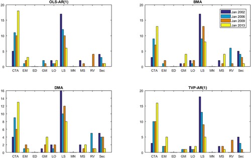
Figure 2. Optimal portfolio composition (t-statistics).

Note: The figure shows the composition of portfolios selected based on t-statistics of expected returns in Jan 2002, Jan 2006, Jan 2009 and Jan 2013. Selected models are OLS-AR(1), BMA, DMA and TVP-AR(1).

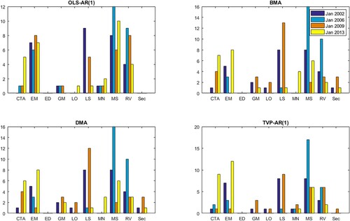
Regarding the portfolios formed based on the forecasts' t-statistics, funds with MS, EM and RV strategies are selected the most. Portfolios selected based on t-statistics are more diversified compared to the portfolios based on expected returns. Interestingly, the ED strategy received a zero weight in all four models, whereas the Sector strategy received a zero weight in the OLS-AR(1) model, but non-zero weights in the other four models. Portfolio composition of the BMA and DMA models seems to show a high degree of similarity when selected based on t-statistics. Finally, the Equity Long/Short strategy attracted a very substantial amount of investment in the crisis period (January 2009). Overall, taking into account model uncertainty in hedge fund return forecasts and portfolio construction is found to lead to a greater degree of diversification when selecting among different trading strategies, compared against the benchmark OLS-AR(1) model. This finding is indicative of the ability of the competing methods to identify the best performing funds from each strategy.

6. Conclusion

In this paper, we jointly investigate the statistical and economic value of incorporating various sources of model risk in forecasting hedge funds returns. Specifically, using an EWMA approach to account for returns' heteroscedasticity, we address parameter uncertainty by applying a time-varying parameter structure while we account for model uncertainty by dynamic model averaging/selection approaches. Our empirical results show that treating for the various sources of model risk significantly improves the forecast accuracy and portfolio performance for both aggregate and fund level returns.

The proposed methods lead to a statistically significant increase in forecast accuracy, as measured by the MSFE, compared to the benchmark OLS-AR(1) model. Specifically, the simplest TVP-AR(1) specification produces the most robust results across the aggregate indices data. However, when we account for the size of underlying funds, we find an increase in the accuracy of the DMA/BMA forecasts. These findings highlight the heterogeneity of the hedge funds investment strategies, which shrinks when we take into account the funds' size. Concerning the decay parameters settings, our results suggest that accuracy benefits more from less persistent volatility, while the coefficients and probability decay rates do not seem to affect the MSFE results significantly.

In the same vein, the economic evaluation results reveal substantial gains from the proposed methods. Furthermore, under the prism of a risk-averse investor, the magnitude of gains is significantly larger than what the statical evaluation suggests. These increased gains are due to the methods' ability to model future uncertainty better than the historical variance of the benchmark. Overall, our findings suggest that TVP-AR(1) specifications provide the most significant gains, while the size effect highlights the need to consider model uncertainty via BMS and DMA specifications. However, a more persistent variance setting is preferable.

Focusing on the individual funds' forecasts, we find that the majority of the competing models select portfolios that significantly outperform the benchmark in average returns and risk-adjusted performance for both evaluation samples. These results provide further support for our approach since we demonstrate that proposed methods provide economic gains by capturing more accurately the predictive density of hedge fund returns.

Disclosure statement

No potential conflict of interest was reported by the author(s).

Additional information

Notes on contributors

Christos Argyropoulos

Christos Argyropoulos received his PhD degree in Finance from the University of Kent, United Kingdom, in 2018. He is a Lecturer (Assistant Professor) in Finance at Essex Business School, University of Essex, UK. He has published in various academic journals in the areas financial time series modelling and forecasting.

Ekaterini Panopoulou

Ekaterini Panopoulou received her PhD degree in Financial Econometrics from the University of Piraeus, Greece, in 2004. She is a Professor of Finance at Essex Business School, University of Essex, UK. She has published in various academic journals in the areas of financial econometrics, time series modelling and forecasting.

Nikolaos Voukelatos

Nikolaos Voukelatos received his PhD in Finance from Lancaster University, UK in 2009. He is a Senior Lecturer in Finance at Kent Business School, University of Kent, UK. He has published in various academic journals in the areas of options, implied information, and asset pricing.

Teng Zheng

Teng Zheng received her PhD degree in Finance from the University of Kent, UK, in 2018. Her thesis topic is “Model Risk in Financial Modelling”. She is currently a VP of the Independent Validation Unit in the Barclays Bank PLC.

Notes

1 ${}^{\ast }$This article represents the views and analysis of the author only and it should not be taken to represent those of her current employer.

1 Key references of this strand of literature include Fung and Hsieh (2001, 2004), Agarwal and Naik (2004), Kosowski, Naik, and Teo (2007), Bali, Gokcan, and Bing (2007), Fung et al. (2008), Jagannathan, Malakhov, and Nomikov (2010), Sadka (2010), Avramov et al. (2011), Bali, Brown, and Caglayan (2011, 2012, 2014), Buraschi, Kosowski, and Sritrakul (2014) and Agarwal, Arisoy, and Naik (2017).

2 The method has been applied recently in several financial research areas, including gold or copper prices forecasting (Aye et al. 2015; Buncic and Moretto 2015; Baur, Beckmann, and Czudaj 2016); house prices forecasting (Bork and Moller 2015; Risse and Kern 2016), bond portfolio strategies selection (Caldeira, Moura, and Santos 2016); stock return forecasting and portfolio construction (Pettenuzzo and Ravazzolo 2016).

3 BMA and BMS specifications are a special case of the DMA and DMS methodologies.

4 Baur, Beckmann, and Czudaj (2016) employ three forgetting factors $\lambda =0.90,0.95,0.99$ in forecasting monthly gold returns and find that DMA or DMS with forgetting factors of at least 0.95 provide more accurate forecasts compared to less flexible alternatives such as BMA or DMA with a forgetting factor fixed to unity, i.e. no forgetting. However, the authors show that a fast rate of forgetting produces instantaneous jumps of the estimated parameters and the posterior predictive model probabilities, which inflates the forecast errors. To this end, they suggest comparing results emerging from the implementation of various forgetting factors. Drachal (2016) focuses on monthly spot oil prices and estimates a total of 121 DMA models based on all combinations of forgetting factors $\alpha ,\lambda =0.90,0.91,\dots ,0.99,1$. The author finds that all DMA models with equal forgetting factors except for the one with $\alpha =\lambda =0.99$ produce larger forecast errors than the naïve forecasting benchmark model. Wang et al. (2016) consider time-varying parameter models to forecast the realized volatility of the S&P 500 index using the heterogeneous autoregressive models for realized volatility. In their experiment, they consider DMA with $\lambda =0.99$ along with constant coefficient models and find that time-varying parameter models have greater forecasting accuracy than models that use constant coefficients. Finally, Catania, Grassi, and Ravazzolo (2019) focus on the predictability of cryptocurrency time series and compare several alternative univariate and multivariate models for point and density forecasting using a forgetting factor of 0.99 in their baseline experiment.

5 Following Koop and Korobilis (2012), we set ${\beta }_0\sim N(0,\frac{\mathrm{var}(r^{t-1})}{\mathrm{var}(z^{t-1})})$ and $H_0=\frac{1}{4}\mathrm{var}(r^{t-1})$.

6 This case refers to linear combinations of predictors.

7 We also considered simple combination schemes, such as the mean, median, trimmed mean. Our results, available from the authors upon request, point to superiority of our time-varying approaches.

8 Joenvaara, Kosowski, and Tolonen (2019), Yin and Zhang (2019), Gao, Haight, and Yin (2019) find that smaller funds yield larger returns. Gao, Haight, and Yin (2019) attribute the recorded performance decline to the diseconomies of scale of large size funds.

9 To address any selection/survival bias, we include in our investment opportunity set both alive and graveyard funds. Graveyard data are sourced from the graveyard database of BarclayHedge. We apply identical data filters as stated in Section 3. All graveyard return series are required to have at least five years of in-sample data prior to 2009, but less than six years of out-of-sample data, depending on when the fund exited the database. This approach results in 395 graveyard funds, post-filtering. Finally, we exclude Funds of Funds from the exercise.

10 The literature hints on the number of funds a FoF typically holds. Specifically, Brown, Gregoriou, and Pascalau (2012) study diversification within FoFs and find that the diversification benefits are maximized when the FoF invests in at most 20 funds. Moreover, they find that adding more funds to the portfolio increases left tail risk and lowers returns. Lhabitant (2006) indicates that the typical number is about 40, while Avramov, Barras, and Kosowski (2013) argue that there is a practical limit to the number of individual funds held by funds of funds and limit the minimum and maximum number of funds in the portfolio to 25 and 75, respectively.

11 Joenvaara, Kosowski, and Tolonen (2019) suggest that realistic investor constraints, such as investors' liquidity constraints, can significantly reduce the recorded performance of hedge funds. While such constraints are essential from the perspective of performance persistence, in our paper we focus on the informational advantage of the proposed specifications and whether such methods could extract performance increments compared to a naïve AR(1) benchmark. Applying the complete set of investor constraints in the spirit of Joenvaara, Kosowski, and Tolonen (2019), in conjunction with our sample size and the data intensity of the suggested specifications, could lead to small sample or selection biases, as the pool of funds in our database would decrease significantly for the most realistic cases. Nevertheless, to emulate broadly such constraints, we impose a one-year rebalancing scheme for our theoretical fund of hedge funds portfolios. By doing so, we restrict our investor to be committed to her selection of funds for the whole year, regardless of a fund offering smaller lock up and redemption periods. Hence, while our portfolios may not be entirely realistic in terms of investors' behavior and practices, they provide a consistent platform for evaluating the proposed portfolios against a similarly defined AR(1) benchmark portfolio.

References

- Agarwal, V., Y. E. Arisoy, and N. Y. Naik. 2017. “Volatility of Aggregate Volatility and Hedge Fund Returns.” Journal of Financial Economics 125: 491–510.
- Agarwal, V., T. Green, and H. Ren. 2018. “Alpha Or Beta in the Eye of the Beholder: What Drives Hedge Funds Flows.” Journal of Financial Economics 127: 417–434.
- Agarwal, V., and N. Y. Naik. 2004. “Risks and Portfolio Decisions Involving Hedge Funds.” Review of Financial Studies 17: 63–98.
- Amenc, N., S. El Bied, and L. Martellini. 2003. “Predictability in Hedge Fund Returns.” Financial Analysts Journal 59: 32–46.
- Avramov, D., L. Barras, and R. Kosowski. 2013. “Hedge Fund Return Predictability Under the Magnifying Glass.” Journal of Financial and Quantitative Analysis 48: 1057–1083.
- Avramov, D., R. Kosowski, N. Y. Naik, and M. Teo. 2011. “Hedge Funds, Managerial Skill, and Macroeconomic Variables.” Journal of Financial Economics 99: 672–692.
- Aye, G., R. Gupta, S. Hammoudeh, and W. J. Kim. 2015. “Forecasting the Price of Gold Using Dynamic Model Averaging.” International Review of Financial Analysis 41: 257–266.
- Bali, T., Y. Atilgan, and O. Demirtas. 2013. Investing in Hedge Funds: A Guide to Measuring Risk and Return Characteristics. Massachusetts, MA: Academic Press.
- Bali, T. G., S. J. Brown, and M. O. Caglayan. 2011. “Do Hedge Funds' Exposures to Risk Factors Predict Their Future Returns?.” Journal of Financial Economics 101: 36–68.
- Bali, T. G., S. J. Brown, and M. O. Caglayan. 2012. “Systematic Risk and the Cross Section of Hedge Fund Returns.” Journal of Financial Economics 106: 114–131.
- Bali, T. G., S. J. Brown, and M. O. Caglayan. 2014. “Macroeconomic Risk and Hedge Fund Returns.” Journal of Financial Economics 114: 1–19.
- Bali, T. G., S. J. Brown, and M. O. Caglayan. 2019. “Upside Potential of Hedge Funds As a Predictor of Future Performance.” Journal of Banking and Finance 98: 212–229.
- Bali, T., S. Gokcan, and L. Bing. 2007. “Value At Risk and the Cross-section of Hedge Fund Returns.” Journal of Banking and Finance 31: 1135–1166.
- Barberis, N. 2000. “Investing for the Long Run when Returns are Predictable.” The Journal of Finance55: 225–264.
- Baur, D. G., J. Beckmann, and R. Czudaj. 2016. “A Melting Pot – Gold Price Forecasts Under Model and Parameter Uncertainty.” International Review of Financial Analysis 48: 282–291.
- Bork, L., and S. V. Moller. 2015. “Forecasting House Prices in the 50 States Using Dynamic Model Averaging and Dynamic Model Selection.” International Journal of Forecasting 31: 63–78.
- Brown, S. J., G. N. Gregoriou, and R. Pascalau. 2012. “Diversification in Funds of Hedge Funds: Is it Possible to Overdiversify?.” The Review of Asset Pricing Studies 2 (1): 89–110.
- Buncic, D., and C. Moretto. 2015. “Forecasting Copper Prices with Dynamic Averaging and Selection Models.” The North American Journal of Economics and Finance 33: 1–38.
- Buraschi, A., R. Kosowski, and W. Sritrakul. 2014. “Incentives and Endogenous Risk Taking: A Structural View on Hedge Fund Alphas.” The Journal of Finance 69: 2819–2870.
- Caldeira, J. F., G. V. Moura, and A. A. Santos. 2016. “Bond Portfolio Optimization Using Dynamic Factor Models.” Journal of Empirical Finance 37: 128–158.
- Campbell, J. Y., and S. B. Thompson. 2008. “Predicting Excess Stock Returns out of Sample: Can Anything Beat the Historical Average?.” Review of Financial Studies 21: 1509–1531.
- Catania, L., S. Grassi, and F. Ravazzolo. 2019. “Forecasting Cryptocurrencies Under Model and Parameter Instability.” International Journal of Forecasting 35 (2): 485–501.
- Cenesizoglu, T., and A. Timmermann. 2012. “Do Return Prediction Models Add Economic Value?.” Journal of Banking and Finance 36: 2974–2987.
- Clark, T. E., and K. D. West. 2007. “Approximately Normal Tests for Equal Predictive Accuracy in Nested Models.” Journal of Econometrics 138 (1): 291–311.
- Drachal, K. 2016. “Forecasting Spot Oil Price in a Dynamic Model Averaging Framework–Have the Determinants Changed Over Time?.” Energy Economics 60: 35–46.
- Eling, M., and R. Faust. 2010. “The Performance of Hedge Funds and Mutual Funds in Emerging Markets.” Journal of Banking and Finance 34: 1993–2009.
- Fung, W., and D. A. Hsieh. 2001. “The Risk in Hedge Fund Strategies: Theory and Evidence From Trend Followers.” The Review of Financial Studies 14: 313–341.
- Fung, W., and D. A. Hsieh. 2004. “Hedge Fund Benchmarks: A Risk-based Approach.” Financial Analysts Journal 60: 65–80.
- Fung, W., D. A. Hsieh, N. Y. Naik, and T. Ramadorai. 2008. “Hedge Funds: Performance, Risk, and Capital Formation.” The Journal of Finance 63: 1777–1803.
- Gao, C., T. D. Haight, and C. Yin. 2019. Size, Age, and the Performance Life Cycle of Hedge Funds. Working Paper.
- Getmansky, M., A. W. Lo, and I. Makarov. 2004. “An Econometric Model of Serial Correlation and Illiquidity in Hedge Fund Returns.” Journal of Financial Economics 74: 529–609.
- Giamouridis, D., and I. D. Vrontos. 2007. “Hedge Fund Portfolio Construction: A Comparison of Static and Dynamic Approaches.” Journal of Banking and Finance 31 (1): 199–217.
- Goetzmann, W., J. Ingersoll, M. Spiegel, and I. Welch. 2007. “Portfolio Performance Manipulation and Manipulation-proof Performance Measures.” Review of Financial Studies 20: 1503–1546.
- Harris, R. D., and M. Mazibas. 2013. “Dynamic Hedge Fund Portfolio Construction: A Semi-parametric Approach.” Journal of Banking and Finance 37: 139–149.
- Jagannathan, R., A. Malakhov, and D. Nomikov. 2010. “Do Hot Hands Exist Among Hedge Fund Managers? An Empirical Evaluation.” The Journal of Finance 65: 217–255.
- Joenvaara, J., R. Kosowski, and P. Tolonen. 2019. “The Effect of Investment Constraints on Hedge Fund Investor Returns.” Journal of Financial and Quantitative Analysis 54: 1539–1571.
- Joenvaara, J., R. Kosowski, and P. Tolonen. 2021. “Hedge Fund Performance: are Stylized Facts Sensitive to which Database One Uses?.” Critical Finance Review 10: 271–327.
- Kandel, S., and R. F. Stambaugh. 1996. “On the Predictability of Stock Returns: An Asset-allocation Perspective.” The Journal of Finance 51: 385–424.
- Keating, C., and W. F. Shadwick. 2002. “A Universal Performance Measure.” Journal of Performance Measurement 6: 59–84.
- Koop, G., and D. Korobilis. 2012. “Forecasting Inflation Using Dynamic Model Averaging.” International Economic Review 53: 867–886.
- Kosowski, R., N. Y. Naik, and M. Teo. 2007. “Do Hedge Funds Deliver Alpha? A Bayesian and Bootstrap Analysis.” The Journal of Financial Economics 84: 229–264.
- Leitch, G., and J. E. Tanner. 1991. “Economic Forecast Evaluation: Profits Versus the Conventional Error Measures.” American Economic Review 81: 580–590.
- Lhabitant, F. S. 2006. Handbook of Hedge Funds. London: John Wiley & Sons.
- Meinhold, R. J., and N. D. Singpurwalla. 1983. “Understanding the Kalman Filter.” The American Statistician 37: 123–127.
- Neely, C. J., D. E. Rapach, J. Tu, and G. Zhou. 2014. “Forecasting the Equity Risk Premium: the Role of Technical Indicators.” Management Science 60: 1772–1791.
- O'Doherty, M. S., N. E. Savin, and A. Tiwari. 2015. “Evaluating Hedge Funds with Pooled Benchmarks.” Management Science 62: 69–89.
- Panopoulou, E., and S. Vrontos. 2015. “Hedge Fund Return Predictability; to Combine Forecasts Or Combine Information?.” Journal of Banking and Finance 56: 103–122.
- Pettenuzzo, D., and F. Ravazzolo. 2016. “Optimal Portfolio Choice Under Decision-based Model Combinations.” Journal of Applied Econometrics 31: 1312–1332.
- Raftery, A. E. 1995. “Bayesian Model Selection in Social Research.” Sociological Methodology 25: 111–164.
- Raftery, A. E., M. Karny, and P. Ettler. 2010. “Online Prediction Under Model Uncertainty Via Dynamic Model Averaging: Application to a Cold Rolling Mill.” Technometrics 52: 52–66.
- RISKMETRICS. 1996. “Technical Document–Fourth Edition.” http://www.riskmetrics.com/system/files/private/td4e.pdf.
- Risse, M., and M. Kern. 2016. “Forecasting House-price Growth in the Euro Area with Dynamic Model Averaging.” North American Journal of Economics and Finance 38: 70–85.
- Sadka, R. 2010. “Liquidity Risk and the Cross-Section of Hedge-Fund Returns.” Journal of Financial Economics 98: 54–71.
- Slavutskaya, A. 2013. “Short-term Hedge Fund Performance.” Journal of Banking and Finance 37: 4404–4431.
- Smith, R., and J. Miller. 1986. “A Non-gaussian State Space Model and Application to Prediction of Records.” Journal of the Royal Statistical Society. Series B (Methodological) 48: 79–88.
- Sortino, F. A., and S. Satchell. 2001. Managing Downside Risk in Financial Markets. Oxford, UK: Butterworth- Heinemann.
- Sortino, F. A., R. van der Meer, and A. Plantinga. 1999. “The Dutch Triangle.” The Journal of Portfolio Management 26: 50–57.
- Stambaugh, R. F. 1999. “Predictive Regressions.” Journal of Financial Economics 54: 375–421.
- Vrontos, I. 2012. “Evidence for Hedge Fund Predictability From a Multivariate Student's T Full-Factor Garch Model.” Journal of Applied Statistics 39: 1295–1321.
- Vrontos, S. D., I. D. Vrontos, and D. Giamouridis. 2008. “Hedge Fund Pricing and Model Uncertainty.” Journal of Banking and Finance 32: 741–753.
- Wang, Y., F. Ma, Y. Wei, and C. Wu. 2016. “Forecasting Realized Volatility in a Changing World: A Dynamic Model Averaging Approach.” Journal of Banking and Finance 64: 136–149.
- Wegener, C., R. von Nitzsch, and C. Cengiz. 2010. “An Advanced Perspective on the Predictability in Hedge Fund Returns.” Journal of Banking and Finance 34: 2694–2708.
- Yin, C., and X. Zhang. 2019. Gambling or De-Risking: Hedge Fund Risk-Taking vs. Management Fees. Working Paper.