International monetary policy and cryptocurrency markets: dynamic and spillover effects

Abstract

Using daily data over the period August 5, 2013 – September 27, 2019, this study investigates the dynamic spillovers between international monetary policies across four major economies (i.e. Eurozone, Japan, UK and US) and three key cryptocurrencies (i.e. Bitcoin, Litecoin and Ripple). In doing so, we apply a Time-Varying Parameter Vector Auto-Regression (TVP-VAR) model, a dynamic connectedness approach and network analysis. The empirical results indicate that cryptocurrency returns and monetary policy spillovers were particularly large when shadow policy rates became negative, moderated during the Fed's ‘tapering process’, and sharpened again more recently as cryptocurrency buoyancy returned. Gross directional spillovers suggest that shadow policy rates have more ‘to give than to receive’, while those from and to cryptocurrency returns are naturally volatile. There is also strong interconnectedness between monetary policy in either the US or the Eurozone and the UK, and between Bitcoin and Litecoin. However, the spillovers across monetary policy and cryptocurrencies tend to be muted. Finally, spillovers were only slightly larger during the Fed's ‘unconventional’ policy compared to the ‘standard’ era, but their composition qualitatively changed over time.

KEYWORDS:

• Monetary policy
• cryptocurrency
• time-variation
• interconnectedness
• spillovers
• international transmission

JEL Codes:

• C32
• C50
• E43
• E52
• G10

1. Introduction

In the aftermath of the global financial crisis, central banks in both developed countries and emerging market economies have deployed a series of unconventional monetary policies (Jawadi et al., 2017; Agnello et al., 2019), whereby the expansion of the monetary authority's own balance sheet is used to support economic activity and promote higher inflation (Blinder, 2000; Bernanke and Reinhart, 2004). These large-scale national policies were quickly transmitted across jurisdictions and a surge in liquidity was globally witnessed (Chen et al., 2016; Tillmann, 2016). Not surprisingly, international monetary policy spillovers became particularly relevant, posing challenges for policymakers (Avdjiev and Hale, 2019; Avdjiev et al., 2020). Thus, understanding their nature and size is crucial.

In this context, abundant liquidity raised concerns about excessive risk-taking with potential disruptions on financial stability (Mostak Ahamed and Mallick 2017a; 2017b; 2019) even though the increased sensitivity of the balance sheets of financial intermediaries to changes in interest rates would warrant a somewhat cautious withdrawal approach (Turner, 2017). Similarly, the extremely accommodative monetary conditions reinforced the role played by the policy toolkit of specialised macro-prudential regulators (Turner, 2018) to the extent that the former might be responsible for large fluctuations of the domestic currency and the emergence of asset bubbles (Tillmann et al., 2019). Among these, cryptocurrencies are the most widely labelled (speculative) bubble (Bouoiyour and Selmi, 2015; Bouoiyour et al., 2016; Selmi et al., 2018), echoing numerous voices from Nobel Prizes (Shiller, 2014; Stiglitz, 2017; Krugman, 2018; Thaler, 2018) and central bank officials (Greenspan, 2013; Carstens, 2017; Constâncio, 2017) to investors (Buffett, 2018; Soros, 2018) and business executives (Dimon, 2017; Ma, 2018), who challenged any interest as investable assets (Dyhrberg et al., 2018). Indeed, being often characterised as digital assets that use encryption to secure transactions, the pricing behaviour of cryptocurrencies typically detaches from commodities (like oil or gold) or traditional financial assets, which explains why investors are attracted by the diversification benefits that they might provide (Baur et al., 2018; Ji et al., 2018; Bouoiyour et al., 2019).

Yet, cryptocurrencies are ‘unique’, as they do not generate cash flows. These virtual currencies rely on decentralised control and require no third-party involvement, being independent of central banks and governments, despite counting on regulated financial institutions to operate (Auer and Claessens, 2018). Thus, in contrast with traditional assets (e.g. bonds, commodities and equities), the standard transmission channels of monetary policy do not apply: in the absence of intrinsic cash flows for investors to discount for or to form expectations about (Lobo, 2000).

Despite this, the empirical evidence on the link between monetary policy and cryptocurrency returns is rather limited and inconclusive: some studies show that (tightening) monetary policy (in China) has a negative effect on cryptocurrency returns (Nguyen et al., 2019); others argue that it depends on the digital asset typology and the (un)conventional nature of policy measures, so (protocol-based) cryptocurrency returns (such as Bitcoin, Litecoin or Ripple) are significantly affected by US monetary policy announcements (Corbet et al., 2020); and some others do not uncover any impact of monetary policy events from major central banks on the Bitcoin price volatility (Vidal-Tomas and Ibañez, 2018). Given the lack of consensus about the response of cryptocurrencies to monetary policy, we aim at filling this literature gap.

Against this backdrop, our contributions are fourfold. First, to the best of our knowledge this is the seminal attempt to examine the dynamic connectedness between international monetary policy and cryptocurrency markets. In this regard, we rely on the innovative Time-Varying Parameter Vector Auto-Regression (TVP-VAR) model developed by Koop and Korobilis (2014) to analyse (the time-varying nature of) the effects of monetary policy on cryptocurrency markets. In this respect, we owe to the work by Antonakakis et al. (2019), who also examine the transmission of international monetary policy spillovers across developed economies by means of a similar framework. The authors find that the size of international monetary policy spillovers has evolved over time, hitting record levels during the global financial crisis of 2008-2009.

Second, we use the TVP-VAR model in conjunction with the dynamic connectedness approach by Diebold and Yilmaz (2009, 2012, 2014). This allows us to distinguish between the dynamics of own shocks and spillovers (i) between international monetary policies; (ii) between cryptocurrency markets; and (iii) across international monetary policy and cryptocurrency markets. Moreover, this combined framework is particularly well-suited to overcome the challenges faced by the dynamic version of the fixed-coefficients VAR model, as it does not require a somewhat arbitrary rolling window size, it is not sensitive to outliers and it does not imply any loss of information (Antonakakis and Gabauer, 2017; Antonakakis et al., 2018, 2019; Gabauer and Gupta, 2018; Korobilis and Yilmaz, 2018). In addition, we build a network analysis (Jacomy et al., 2014) to quantify and visualise the role played by international monetary policy in shaping cryptocurrency returns.

Third, we investigate the asymmetry of such spillovers by distinguishing between conventional and unconventional monetary policy regimes in the US. As noted by Corbet et al. (2020), this consideration is important. Indeed, the US monetary policy is a major source of global risk appetite and financial spillovers (Georgiadis, 2016; Georgiadis and Mehl, 2016). Besides, the US is a dominant transmitter of international monetary policy spillovers (Avdjiev et al., 2020), a feature that has not significantly changed between unconventional and conventional eras (Antonakakis et al., 2019).

Fourth, we use daily data to assess the dynamics and impact of monetary policy (spillovers). While the majority of studies on the macroeconomic impact monetary policy primarily rely on low-frequency data (Claessens et al., 2016), Nakamura and Steinsson (2018a, 2018b) emphasise that high-frequency data is of crucial importance for the accuracy of the results. Thus, we consider the daily shadow short-rate by Krippner (2013, 2015), which is the nominal interest rate that would prevail in the absence of its effective lower bound. This synthetic indicator provides a common metric for the monetary policy stance, so it also has the advantage of allowing a comparison across conventional and unconventional regimes.

Using data for the shadow short-rates of four major developed economies (Eurozone, Japan, UK and US) and the price of three key cryptocurrencies (Bitcoin, Litecoin and Ripple) over the period August 5, 2013 – September 27, 2019, we find a reasonable degree of connectedness: approximately one quarter of the forecast error-variance in all variables comes from spillovers. Moreover, we show that interconnectedness has evolved over time. Thus, cryptocurrency returns and monetary policy spillovers were particularly large when central banks embarked quantitative easing programmes and shadow policy rates hit negative territory. As the Fed began the so-called ‘tapering process’, spillovers started to decrease despite some occasional spikes surrounding monetary policy actions. Finally, spillovers rose sharply since mid-2018, reflecting the fall in shadow policy rates and a cryptocurrency buoyancy revival.

Additionally, we show that gross directional spillovers from shadow policy rates in the US and the Eurozone to all other variables clearly exhibit a cycle pattern. These correspond to the easing, normalisation and tightening cycles of different monetary policy regimes. However, gross directional spillovers of shadow policy rates from all others have remained low (at around 2%-6%) throughout the sample period, which reveals that they have more ‘to give than to receive’. By contrast, gross directional spillovers from and to cryptocurrency returns have been characterised by occasional spikes. This speaks to the clustering and meteoric cryptocurrency price volatility (Bariviera et al., 2017; Urquhart, 2017; Auer, 2019).

Regarding net directional spillovers, the empirical evidence corroborates the view of the lack of monetary policy synchronisation over the past years, as a reflex of a different positioning in the business cycle. Therefore, the US is generally a net transmitter of shocks, the Eurozone and the UK are both net transmitters and receivers of shocks, and Japan remains a net receiver of shocks. Put it differently, the announcement of policy measures by a specific central bank typically meant that it became a net transmitter of shocks, while other central banks turned net receivers of shocks. Concerning the net spillovers of cryptocurrency returns, they have been positive for Bitcoin and Litecoin, and negative for Ripple. Thus, while the former have been net transmitters of shocks, the latter has been a net receiver.

Our network analysis shows strong interconnectedness between monetary policy (in particular, between either the US or the Eurozone and the UK). There are also strong spillovers between cryptocurrency returns (especially, between Bitcoin and Litecoin). However, the spillovers across monetary policy and cryptocurrencies appear muted.

Finally, when we evaluate the main findings through the lens of the US (un)conventional monetary policy eras, the results suggest only a slightly larger spillovers in ‘non-standard’ times compared to those in ‘normal’ periods. However, net directional spillovers shifted from positive to negative in the case of the Eurozone, and from negative to positive in the case of the UK. This suggests that the Eurozone was an important transmitter of monetary spillovers during the first half of the sample period, while the UK became a key source of monetary spillovers afterwards, possibly reflecting the Brexit referendum in 2016 and the corresponding elevated uncertainty. Moreover, they were nil for Litecoin during US unconventional monetary policy and for Bitcoin during US conventional monetary policy.

All in all, our results can prove useful for investors engaging in asset allocation and risk management, who should factor in monetary spillovers in their portfolio decisions. Additionally, as cryptocurrency returns seem relatively immune to such spillovers, they might offer diversification benefits to investors who are eager to take speculative positions. From a policy perspective, while monetary spillovers pose challenges for policymakers in each jurisdiction, they also offer ample opportunities for international policy coordination.

The remainder of the paper is organised as follows. Section 2 provides a brief review of the literature. Section 3 describes the econometric methodologies used in the analysis. Section 4 presents the data and discusses the empirical results. Section 5 concludes.

2. Literature review

Our paper is related with four strands of the literature. The first one lies at the heart of the discussion about international monetary spillovers. In this context, Chen et al. (2016) rely on a global vector error-correction model to study the international effects of US quantitative easing. They find that the impact on emerging markets is larger than for advance economies. Tillman et al. (2019) also detect substantial, asymmetric and nonlinear spillovers from US monetary policy to emerging markets. Belke et al. (2018) and Galariotis et al. (2018) investigate the connectedness between bond yields. Claus et al. (2016) use a constant parameter latent factor model, and find spillovers across monetary policies between the US and Japan, with the effect being stronger during unconventional monetary policy regimes. Liu et al. (2018) analyse the interaction between monetary policy decisions of major central banks in the US, the UK and the Eurozone. Using the dynamic (i.e. rolling-window based) version of the connectedness approach of Diebold and Yilmaz (2009, 2012, 2014), Belke and Dubova (2018) assess the spillovers between shadow rates and global asset markets.

The second line of investigation deals with a range of cryptocurrency dimensions (Corbet et al., 2020), including bubbles and inefficiencies (Bouoiyour and Selmi, 2015; Brandvold et al., 2015; Cheah and Fry, 2015; Bouoiyour et al., 2016, 2019; Nadarajah and Chu, 2017; Selmi et al., 2018; Corbet et al., 2019; Sensoy, 2019), price clustering and volatility (Bariviera et al., 2017; Urquhart, 2017; Auer, 2019) or jurisdictional regulation (Fry, 2018; Auer and Claessens, 2018). The unique technology (Böhme et al., 2015) and characteristics as traded assets (Corbet et al., 2018) that use peer-to-peer networks to overcome the double-spending problem (Dwyer, 2015; Auer, 2019), as well the exceptional fraud levels related to cryptocurrencies (Gandal et al., 2018), have also been studied.

The third avenue of related research looks at the interaction between monetary policy and cryptocurrency markets. In this field, Demir et al. (2018) uncover a negative impact of economic policy uncertainty on Bitcoin returns. Nguyen et al. (2019) use the Generalised Method of Moments (GMM) estimator by Blundell and Bond (1998) in a(n) (otherwise standard) return equation to evaluate the presence of asymmetry in the response of four major cryptocurrency markets (i.e. Bitcoin, Ethereum, Litecoin and Ripple) to a tightening or easing of monetary policy in China and the US. They show that while cryptocurrency returns do not significantly change in response to the level of policy rates in both countries, a tightening of Chinese policy rates leads to a significant rise in cryptocurrency returns. This corroborates the existence of capital flights from equities to cryptocurrencies when such monetary policy actions in China occur. Corbet et al. (2020) use Exponential Generalised Autoregressive Conditional Heteroscedasticity (EGARCH) models to investigate (asymmetric) volatility spillover and feedback effects of US standard and non-standard monetary announcements on 58 digital assets (classified as currencies, protocols, and decentralised applications). They find that while there are significant spillovers in the case of currency-based (and mineable) digital assets, the empirical evidence does broadly not reveal spillover and feedback effects for application or protocol-based (and non-mineable) digital assets. By contrast, Vidal-Tomas and Ibañez (2018) present an event study with monetary policy and Bitcoin news that employs several auto-regressive-component GARCH (AR-CGARCH) model to assess semi-strong efficiency in Bitcoin. The authors show that Bitcoin does not respond to monetary policy events (which are public financial information) from four major central banks (i.e. the Bank of England, the Bank of Japan, the European Central Bank and the Federal Reserve System). Therefore, Bitcoin is semi-strong form inefficient vis-à-vis monetary policy news.

Finally, the fourth strand of the related literature highlights the advantage of cryptocurrencies in international diversification. In particular, being somewhat disconnected from economic fundamentals and the global financial system, cryptocurrencies can be a relevant portfolio diversifier for both alternative and conventional assets (Bouri et al., 2017; Baur et al., 2018). In this context, Corbet et al. (2018) look at the link between three cryptocurrencies (i.e. Bitcoin, Ripple and Litecoin) and several financial assets. The authors show that the idiosyncratic risk of the cryptocurrency market complicates its use as a hedge. Moreover, even though cryptocurrencies provide diversification benefits over the short-term, the fact that they are connected with each other and other economic and financial assets makes them a new investment class on their own. Bouri et al. (2017), Baur et al. (2018), Corbet et al. (2018), Klein et al. (2018) and Guesmi et al. (2019) provide evidence that is not consensual about the hedging ability of Bitcoin vis-à-vis unfavourable equity fluctuations. Sensoy (2019) finds a diversified efficiency degree among different currency Bitcoin markets, which points to arbitrage opportunities and portfolio diversification gains (Makarov and Schoar, 2020). Cryptocurrencies also appear to deliver portfolio diversification benefits in emerging markets (Omane-Adjepong and Alagidede, 2020), vis-à-vis traditional assets (Platanakis and Urquhart, 2020) or relative to domestic currencies (Kyriazis, 2019). Qarni and Gulzar (2021) uncover significant portfolio diversification benefits of Bitcoin for alternative currency foreign exchange portfolios, showing that the former can be used as a hedge against the risk associated with the latter. Finally, Hatemi-J (2021) analyse the potential portfolio diversification benefits of Bitcoin relative to bonds, equities and the US dollar. They show significant advantages, in terms of return per unit risk, only if portfolios are constructed by means of combining risk and return instead of minimising variance.

As can be inferred from above, there are only a few studies that examine the response of cryptocurrencies (which do not intrinsically generate cash flows) to monetary policy events and the empirical evidence therein is inconclusive. For these reasons, the impact of monetary policy on cryptocurrency markets remains largely unanswered. More importantly, almost all existing works implicitly assume that the relationship (and the spillovers) between monetary policy and cryptocurrencies is time-invariant (i.e. static) in nature. Given the number and diversity of monetary policy actions and turbulence events observed in the recent past, such assumption is questionable implying that the use of average estimates would mask important information on the pattern and directional effects. Therefore, our paper examines the dynamic connectedness and spillovers across international monetary policy and cryptocurrencies using a TVP-VAR approach. As such, it fills a key gap in the literature.

3. Econometric methodology

3.1 Dynamic effects of international monetary policy

We assess the dynamic effects of international monetary policy on cryptocurrency markets by estimating a Time-Varying Parameter Vector Auto-Regression (TVP-VAR) model. Thus, along the lines proposed by Koop and Korobilis (2014), we allow the VAR coefficients to vary over time and estimate them via a Kalman Filter equation with a lag-order of one.

This framework substantially improves vis-à-vis the ‘dynamic’ version of the standard (i.e. fixed-coefficients) VAR model, which is estimated on the basis of an often arbitrary rolling-window size. Indeed, the strong flexibility of the TVP-VAR model allows all parameters to be time-varying. As such, potential parameter changes are accurately determined. This is also a key assumption that adheres to the empirical observation of time-variation in the joint dynamics of models that embed both financial and macroeconomic data like ours (Banerjee et al., 2008; Breitung and Eickmeier, 2011; Bates et al., 2013; Koop and Korobilis, 2014). Moreover, as there is no loss of valuable observations and the methodology is immune to the presence of outliers compared to the spillover approach based on the fixed-coefficient VAR framework,¹ the odds of erratic or flattened parameters are low in the TVP-VAR model (Antonakakis et al., 2020). As a result, it can be used in association with the framework put forward by Diebold and Yilmaz (2009, 2012, 2014) to construct spillover indices and examine the dynamic interconnectedness between international monetary policy and cryptocurrency returns.²

Our TVP-VAR model can be written as follows, (1) $\begin{array}{rl}{\mathit{Y}}_t& ={\mathbf{\Psi }}_t{\mathit{Y}}_{t-1}+{\mathit{\xi }}_t,{\mathit{\xi }}_t|{\mathbf{\Omega }}_t\sim \mathrm{N}(0,{\mathbf{\Lambda }}_{\text{t}}),\end{array}$(1) (2) $\begin{array}{rl}{\mathbf{\Psi }}_t& ={\mathbf{\Psi }}_{t-1}+{\mathit{\eta }}_t,{\mathit{\eta }}_t|{\mathbf{\Omega }}_t\sim \mathrm{N}(0,{\mathbf{\Gamma }}_{\text{t}}),\end{array}$(2) where ${\mathit{Y}}_t$ is an $N\times 1$ vector of endogenous variables, ${\mathit{Y}}_{t-1}$ is an $Np\times 1$ lagged conditional vector, ${\mathbf{\Psi }}_t$ is an $N\times Np$ time-varying coefficient matrix, and ${\mathit{\xi }}_t$ is an $N\times 1$ vector of error disturbance terms with an $N\times N$ time-varying variance-covariance matrix, ${\mathbf{\Lambda }}_{\text{t}}$. The parameters ${\mathbf{\Psi }}_t$ depend on their own past values, ${\mathbf{\Psi }}_{t-1}$, and an $N\times Np$ error disturbance matrix, ${\mathit{\eta }}_t$, with an $Np\times Np$ variance-covariance matrix, ${\mathbf{\Gamma }}_{\text{t}}$.

In this setup, ${\mathit{Y}}_t=[\mathit{C}{\mathit{C}}_{\mathit{t}},\mathit{S}\mathit{S}{\mathit{R}}_{\mathit{t}}]{}^{\mathrm{\prime }}$, where $\mathit{C}{\mathit{C}}_t=[BT{C}_t,XR{P}_t,LT{C}_t{]}^{{}^{\mathrm{\prime }}}$ is a vector of cryptocurrencies (i.e. Bitcoin (BTC), Ripple (XRP) and Litecoin (LTC)), $\mathit{S}\mathit{S}{\mathit{R}}_t=[US.SS{R}_t,EZ.SS{R}_t,JP.SSR,UK.SSR]{}^{\mathrm{\prime }}$ is a vector of shadow short-rates capturing the monetary policy stance in the US, the Eurozone, Japan and the UK, respectively.

In the model, there are only two input parameters: (i) the H-step ahead forecast horizon; (ii) the lag length, p, of the TVP-VAR model. The H-step forecast horizon is set to 10 days, as it effectively captures the sort-term impact of international monetary policy on cryptocurrency returns.³ The lag length of the VAR model corresponds to the optimal lag length based on the Bayesian information criterion (BIC), and it is set to two.

3.2 Spillover effects of international monetary policy

The time-varying coefficients and error covariances are used to estimate the spillover indices of Diebold and Yilmaz (2009, 2012, 2014). These are based on generalised impulse response functions (GIRF) and generalised forecast error variance decompositions (GFEVD) developed by Koop et al. (1996) and Pesaran and Shin (1998).

To calculate the GIRF and GFEVD, we express the TVP-VAR model, described by the system (1)-(2), in its moving average representation as follows: (3) ${\mathit{Y}}_t={\mathrm{\Theta }}_t{\mathit{\xi }}_t$(3) where ${\mathrm{\Psi }}_t=[{\mathrm{\Psi }}_{1,t},\dots ,{\mathrm{\Psi }}_{p,t}]{}^{\mathrm{\prime }}$, ${\mathrm{\Theta }}_t=[{\mathrm{\Theta }}_{1,t},\dots ,{\mathrm{\Theta }}_{p,t}]{}^{\mathrm{\prime }}$, and ${\mathrm{\Psi }}_{i,t}$ and ${\mathrm{\Theta }}_{i,t}$ are $N\times N$ parameter matrices, such that ${\mathrm{\Theta }}_{0,t}=\mathit{I},{\mathrm{\Theta }}_{i,t}=0$ for i <0, and ${\mathrm{\Theta }}_{i,t}={\mathrm{\Psi }}_{1,t}{\mathrm{\Theta }}_{i-1,t}+\dots +{\mathrm{\Psi }}_{p,t}{\mathrm{\Theta }}_{i-p,t}$.

In this setup, spillovers (or cross variance shares) correspond to fractions of the H-step-ahead error variances in forecasting a specific variable i of the vector ${\mathit{Y}}_t$ that are due to shocks in variable j = 1, 2, . . ., N, such that $j\ne i$, while the own variance shares are fractions of the H-step-ahead error variances in forecasting a specific variable i of the vector ${\mathit{Y}}_t$ that are due to own shocks, for i = 1, 2, . . ., N.

The H-step ahead forecast error is the difference between the actual value, ${\mathit{Y}}_{t+H}$, and the prediction of the future value, $E_t{\mathit{Y}}_{\text{t}+\text{H}}$. Similarly, the generalised impulse-response function (GIRF) represents the response of all variables following a shock in variable i. Thus, it is the difference between the H-step-ahead forecast where variable i is shocked and the H-step-ahead forecast where variable i is not shocked, and can be computed as (4) $GIR{F}_t(H,{\delta }_{j,t},{\mathit{\Omega }}_t)=E_t({\mathit{Y}}_{t+H}|{\mathit{\xi }}_{j,t}={\delta }_{j,t},{\mathit{\Omega }}_t)-E_t({\mathit{Y}}_{t+H}|{\mathit{\Omega }}_t)$(4) where $H$ represents the forecast horizon, $a_{j,t}$ the selection vector with one as the j^th element and zero otherwise, and ${\mathbf{\Omega }}_t$ the information set until t.

Next, we calculate the generalised H-step-ahead forecast error-variance decomposition (GFEVD), ${\mathit{\lambda }}_{j,t}^g(H)$, for H = 1, 2, . . ., as: (5) ${\mathit{\lambda }}_{j,t}^g(H)={\mathrm{\Lambda }}_{\text{jj},\text{t}}^{-\frac{1}{2}}{\mathrm{\Theta }}_{H,t}{\mathbf{\Lambda }}_{\text{t}}{\xi }_{j,t}=\frac{{\mathrm{\Theta }}_{H,t}{\mathit{\Lambda }}_t{\xi }_{j,t}}{\sqrt{{\mathrm{\Lambda }}_{jj,t}}}\frac{a_{j,t}}{\sqrt{{\mathrm{\Lambda }}_{jj,t}}}$(5) where ${\mathbf{\Lambda }}_{\text{t}}$ is the $N\times N$ time-varying variance-covariance matrix of the vector of error disturbance terms ${\mathit{\xi }}_t$, $\sqrt{{\mathrm{\Lambda }}_{jj,t}}$ is the standard deviation of the error term for the j^th equation. The GFEVD can be interpreted as the fraction of the variation of other variables that can be explained by a shock to a specific variable.

In the computation of the spillover index, we normalise each entry of the variance decomposition matrix, so that each row sums up to one, that is, all variables jointly explain 100% of variable’s i generalised forecast-error variance. This is calculated as follows (6) ${\tilde{\lambda }}_{ij,t}^g(H)=\frac{{\sum }_{t=1}^{H-1}{\mathit{\lambda }}_{ij,t}^{2,g}}{{\sum }_{j=1}^N{\sum }_{\mathit{t}=1}^{\mathit{H}-1}{\mathit{\lambda }}_{ij,t}^{2,g}}$(6) which implies that $\sum _{j=1}^N{\tilde{\lambda }}_{ij,t}^N(H)=1$ and $\sum _{i,j=1}^N{\tilde{\lambda }}_{ij,t}^N(H)=N$.

Therefore, the total spillover index that measures the contribution of spillovers of shocks to the total forecast error-variance can be expressed as: (7) $S_t^g(H)=\frac{{\sum }_{i,j=1,i\ne j}^N{\tilde{\lambda }}_{ij,t}^g(H)}{{\sum }_{i,j=1}^N{\tilde{\lambda }}_{ij,t}^g(H)}\cdot 100=\frac{{\sum }_{i,j=1,i\ne j}^N{\tilde{\lambda }}_{ij,t}^g(H)}{N}\cdot 100,$(7)

The gross directional spillovers received by variable i from all other variables j are computed as: (8) $S_{i.,t}^g(H)=\frac{{\sum }_{j=1,i\ne j}^N{\check{\lambda }}_{ij,t}^g(H)}{{\sum }_{i=1}^N{\check{\lambda }}_{ij,t}^g(H)}\cdot 100.$(8)

Similarly, the gross directional spillovers transmitted by variable i to all other variables j are obtained as: (9) $S_{.i,t}^g(H)=\frac{{\sum }_{j=1,i\ne j}^N{\check{\lambda }}_{ji,t}^g(H)}{{\sum }_{j=1}^N{\check{\lambda }}_{ji,t}^g(H)}\cdot 100.$(9)

Net directional spillovers from variable i to all other variables j, which tells us how much each variable i contributes to other variables j, in net terms, are defined as (10) $S_{i,t}^g(H)=S_{.i,t}(H)-S_{i.,t}(H).$(10) If net directional spillovers from variable i to all other variables j is positive (negative), this implies that variable i impacts more (less) than is influenced by the network.

Finally, net pairwise spillovers, i.e. the difference between gross shocks transmitted from variable i to variable j and those transmitted from j to i, are measured as: (11) $S_{ij,t}^g(H)=\left(\frac{{\check{\lambda }}_{ji,t}^g(H)}{{\sum }_{i,k=1}^N{\check{\lambda }}_{ik,t}^g(H)}-\frac{{\check{\lambda }}_{ij,t}^g(H)}{{\sum }_{j,k=1}^N{\check{\lambda }}_{jk,t}^g(H)}\right)\cdot 100=\left(\frac{{\check{\lambda }}_{ji,t}^g(H)-{\check{\lambda }}_{ij,t}^g(H)}{N}\right)\cdot 100.$(11)

3.3 Network analysis

Following the construction of spillover indices, we illustrate the interconnectedness by applying the ForceAtlas2 algorithm developed by Jacomy et al. (2014). Specifically, we calculate nodes and edges, describing the pairwise directional connectedness obtained from spillover indices.

In a system with k variables, each variable has k-1 edges. As such, for the entire system, there will be k²-kedges since the pairs to the own node are of no use. The information generated by the network analysis is based on the variance decomposition function from the TVP-VAR model estimated in Section 3.1. In this context, each pairwise directional connectedness is illustrated by the edge size and the edge colour.

4. Empirical results

4.1 Data

We use daily closing price data for major cryptocurrencies, i.e. Bitcoin (BTC), Ripple (XRP) and Litecoin (LTC).⁴ The continuously compounded cryptocurrency returns are computed as the first-differences of the logs of the price series.

We also gather daily data for the shadow short-rates (i.e. shadow policy rates) of major developed economies, namely, the US ($US.SSR$), the Eurozone ($EU.SSR$), Japan ($JP.SSR$) and the UK ($UK.SSR$). These are synthetic indicators of (un)conventional monetary policy actions (Krippner, 2013; Lombardi and Zhu, 2014; Christensen and Rudebusch, 2016; Wu and Xia, 2016), and provide an adequate characterisation of the monetary policy stance in times of ‘zero’ or ‘near-zero’ policy rates. International shadow short-rates are sourced from the website of the Reserve Bank of New Zealand.⁵ They are estimated from two-factor shadow/lower-bound term structure models (SLMs), which are robust compared to three-factor SLMs (Krippner, 2015). Thus, shadow short-rates are especially important to monitor and quantitatively evaluate non-standard monetary policy conditions. To ensure stationarity, shadow short-rates are expressed in first-differences.

Finally, the sample period is August 5, 2013 – September 27, 2019, as determined by the data availability.⁶ In particular, while the starting date is defined in accordance with the data available for cryptocurrencies, the ending date is set in accordance with the data available for shadow short-rates.

Table 1 provides a summary of the descriptive statistics for all variables included in the study. As can be seen in the upper panel of this table, average cryptocurrency returns are slightly larger for Bitcoin than for Ripple and Litecoin. Average shadow short-rates are positive in the US and the UK and negative for the Eurozone and Japan. No variable is normally distributed, as corroborated by the Jarque-Bera (JB) tests. The unit-root tests by Stock et al. (1996) (ERS) indicate that all variables are stationary. With the exception of the shadow short-rates of the US and Japan, the kurtosis coefficients are well above 3, which implies that they are leptokurtic.

Table 1. Descriptive statistics.

	BTC	XRP	LTC	US.SSR	EU.SSR	JP.SSR	UK.SSR
Mean	0.003	0.002	0.002	0.003	−0.003	−0.003	0.003
Variance	0.003	0.007	0.006	0.000	0.000	0.000	0.001
Maximum	0.521	0.750	0.800	0.097	0.137	0.050	0.159
Minimum	−0.266	−0.512	−0.513	−0.087	−0.037	−0.080	−0.141
Skewness	0.461	1.672	1.686	0.161	2.005	0.201	0.980
Kurtosis	11.363	14.795	19.218	2.503	6.187	2.916	7.985
JB	8686***	15377***	25444***	425***	3633***	578***	4518***
ADF	−8.02***	−8.22***	−8.13***	−8.08***	−4.39***	−4.53***	−7.48***
ERS	−10.32***	−2.07**	−10.626***	−6.564***	−3.437***	−4.066***	−2.192**
Q(20)	25.716***	62.761***	31.801***	1945.376***	9625.899***	6006.911***	3434.099***
Q2(20)	2.859	42.684***	149.113***	246.789***	1908.259***	289.086***	720.376***
ARCH(20)	71.772***	116.729***	126.022***	35.075***	209.153***	56.481***	38.451***
Correlation Matrix
BTC	1
XRP	0.381	1
LTC	0.653	0.361	1
US.SSR	−0.051	−0.024	−0.028	1
EU.SSR	−0.039	0.006	−0.004	0.167	1
JP.SSR	−0.05	−0.031	−0.021	−0.092	−0.002	1
UK.SSR	−0.014	−0.003	−0.037	0.406	0.273	−0.086	1

Notes: This Table shows descriptive statistics and correlation coefficients of the variables under consideration. The returns of cryptocurrencies are estimated as the first-differences of the logs of Bitcoin (BTC), Ripple (XRP) and Litecoin (LTC) price indices. In addition, the shadow short rates (SSR) for the US (US.SSR), the Eurozone (EU.SSR), Japan (JP.SSR) and the UK (UK.SSR) are presented in first-differences to ensure data stationarity. JB is the Jarque-Bera test for Normality, Q(20), and Q²(20) is the Ljung–Box statistic for serial correlation in raw series and squared residuals, respectively. ARCH (20) tests Engle's ARCH effects up to 20 lags. ADF is the Augmented Dickey–Fuller unit root test. ERS is the ADF-GLS unit root test by Stock et al. (1996). Both test the stationarity properties of the series under considerations, and the appropriate lag orders are chosen in accordance with the (minimum value of the) Bayesian Information Criterion (BIC)et al.. ***, ** indicate significance at the 1% and 5% level, respectively.

The lower panel of Table 1 presents the unconditional correlations. As expected, the correlation among cryptocurrency returns is high and positive, especially between Bitcoin (BTC) and Litecoin (LTC). This corroborates the strong interconnectedness between cryptocurrencies (Corbet et al., 2018). With regard to the co-movement among shadow short-rates, it is positive and relatively large between the US and the UK and, less so, between the US and the Eurozone. This comes as no surprise in light of the ‘secular’ downward trend in real interest rates and their international co-movement (Summers, 2014; Eichengreen, 2015; Hall, 2016). Shadow rates in Japan display a negative correlation with other shadow rates. Finally, while shadow short-rates and cryptocurrency returns typically exhibit a low correlation, this tends to be negative, suggesting that monetary policy tightening (easing) has a negative (positive) effect on cryptocurrency returns (Vidal-Tomas and Ibañez, 2018; Nguyen et al., 2019; Corbet et al., 2020). In a low interest rate environment, this points to a ‘search-for-yield’ behaviour by investors and reinforces the view of some diversification gains provided by cryptocurrencies in addition to portfolios consisting of alternative and conventional assets (Bouri et al., 2017; Baur et al., 2018).

4.2 Full sample results

We start by calculating the static spillovers between international monetary policy and cryptocurrency returns over the full sample period. Specifically, we estimate the TVP-VAR model developed by Koop and Korobilis (2014) and rely on the generalised forecast-error variance decompositions (GFEVD) to calculate the average spillover indices proposed by the connectedness approach of Diebold and Yilmaz (2009, 2012, 2014).⁷

Table 2 displays a summary of the main findings for the full sample. As can be seen, the total connectedness index (TCI) is 24.86%, that is, close to one fourth of the forecast error-variance in all variables comes, on average, from: (i) the international spillovers of monetary policy; (ii) the spillovers between monetary policy and cryptocurrency returns; and (iii) the spillovers among cryptocurrency markets.

Table 2. Connectedness – Full sample.

	BTC	XRP	LTC	US.SSR	EU.SSR	JP.SSR	UK.SSR	FROM others
BTC	62.74	9.39	27.19	0.23	0.14	0.19	0.13	37.26
XRP	11.51	77.75	10.22	0.07	0.20	0.10	0.15	22.25
LTC	27.31	8.86	63.13	0.05	0.30	0.06	0.28	36.87
US.SSR	0.05	0.05	0.01	76.44	8.23	0.19	15.03	23.56
EU.SSR	0.21	0.14	0.17	9.00	77.82	0.26	12.41	22.18
JP.SSR	0.29	0.04	0.12	2.59	2.30	93.25	1.41	6.75
UK.SSR	0.37	0.10	0.19	12.90	11.57	0.10	74.77	25.23
TO others	39.75	18.57	37.90	24.84	22.75	0.89	29.41	174.11
Net spillovers	2.49	−3.68	1.03	1.28	0.56	−5.86	4.18	TCI = 24.87%

Notes: This Table summarises the empirical results of the total, directional and pairwise spillovers. They are based on the generalised forecast-error variance decomposition (GFEVD) obtained from the estimation of a TVP-VAR model of order 2 and 10-step ahead forecasts. The lag length is selected in accordance with the Bayesian information criterion (BIC). The sample period is August 5, 2013 – September 27, 2019. ‘TO' directional spillovers correspond to the off-diagonal column sums (labelled contributions TO others), i.e. spillovers from variable i to all variables j. 'FROM' directional spillovers denote the off-diagonal row sums (labelled contributions FROM others), i.e. spillovers from all variables j to variable i. Net spillovers ('NET') are simply the "from" minus "to" differences. The total spillover index, which appears in the lower right corner of the Table, is approximately the grand off-diagonal column sum (or row sum) relative to the grand column sum including the diagonals (or row sum including diagonals), expressed as a percentage.

The ‘To’ row reveals that, among shadow short-rates, the largest gross directional spillovers to others accrue to the UK (29.4%) and the US (24.8%), being followed by the Eurozone (22.8%). By contrast, gross directional spillovers from the shadow short-rate of Japan to others are negligible (0.9%). As for cryptocurrency returns, the largest gross directional spillovers to others are attributed to Bitcoin (39.8%) and Litecoin (37.9%).

Looking at the ‘‘directional from others’’ column, we find that: (i) among monetary policy, the largest gross directional spillovers from others are observed for the UK (25.2%), while the smallest gross directional spillovers from others are recorded for Japan (6.85%); and (ii) among cryptocurrency returns, the lowest gross directional spillovers from others can be attributed to Ripple (22.3%).

Finally, we turn to the net directional spillovers measures. As can be seen, they range between −5.9% (Japan) and 4.2% (UK) among shadow short-rates. For cryptocurrency returns, net directional spillovers lay between −3.7% (Ripple) and 2.5% (Bitcoin). This result is in accordance with the leading and dominant role played by Bitcoin, and can be explained by its attractiveness, computer programming attention, energy prices and user anonymity (Kristoufek, 2015; Yelowitz and Wilson, 2015; Li and Wang, 2017). Moreover, net directional spillovers are negative only for Ripple and Japan’s shadow short-rate. Hence, these are net receivers of spillovers. By contrast, Litecoin and the US shadow short-rate are net transmitters of shocks to other variables in the system (their net directional spillovers are 1% and 1.3%, respectively) but to a lesser extent than the UK shadow short-rate and the Bitcoin (with net directional spillovers of 4.2% and 2.5%, respectively).

In Figure 1, we present the time-varying total connectedness (spillover) index, which is based on the generalised forecast-error variance decomposition (GFEVD) obtained from the estimation of the TVP-VAR model of order 2.

Figure 1. Dynamic total spillover index.

Notes: This Figure displays the time-varying behaviour of the total connectedness index between international monetary policy and cryptocurrency returns. It is based on the generalised forecast-error variance decomposition (GFEVD) obtained from the estimation of a TVP-VAR model of order 2 and 10-step ahead forecasts. The sample period is August 5, 2013 – September 27, 2019. The lag length is selected in accordance with the (minimum value of the) Bayesian information criterion (BIC).

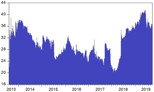
Three striking phases can be detected. First, the spillovers were relatively large (standing at around 35%) at the beginning of the sample period (i.e. 2013-2014), when shadow policy rates in major economies were negative and quantitative easing programmes launched by central banks were largely in place. Cryptocurrency prices also hit record high levels in this phase. Second, the spillovers initiated a downward trend afterwards, to reach a minimum of close to 20% towards the end of 2017, albeit this dynamic is characterised by occasional spikes. During this phase, the Fed started the so-called ‘tapering process’ in December 2013 and ended its large-scale asset purchase programme in October 2014. In addition, it implemented some interest rate hikes in the context of Federal Open Market Committee (FOMC) actions. For instance, towards the end of 2016 and the beginning of 2017, government bond yields started to rise as a reflex of the normalisation of the Fed’s balance sheet. Simultaneously, cryptocurrencies exhibited some price spikes in this period, namely, in mid-2015 and late 2017. Finally, in the third phase, spillovers sharply rose at the end of 2017 and reach a record high level of above 40% in mid-2018, remaining elevated since then. During this period, cryptocurrency prices first hit historically high levels and then sharply declined in 2018. By contrast, shadow policy rates started to fall in the Eurozone (and, similarly, in the US towards the end of 2019).

Figure 2 plots the gross directional spillovers from each underlying variable to all other variables over time. It can be seen that spillovers from cryptocurrency returns to all other variables have typically fallen until late 2017, with occasional upward spikes that reflect episodes of price volatility. Then, they started to rise due to the acute fall in the prices of cryptocurrencies since December 2017 and the increase in the number of cyber-attacks (Bouoiyour et al., 2015) that halted cryptocurrency trading in 2018.

Figure 2. Dynamic gross directional spillovers TO others.

Notes: This Figure displays the time-varying behaviour of the gross directional spillovers from each underlying variable TO all other variables. It is based on the generalised forecast-error variance decomposition (GFEVD) obtained from the estimation of a TVP-VAR model of order 2 and 10-step ahead forecasts. The sample period is August 5, 2013 – September 27, 2019. The lag length is selected in accordance with the Bayesian information criterion (BIC).

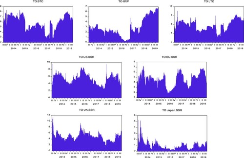
By contrast, the spillovers from shadow policy rates to all other variables clearly exhibit a cycle pattern in the US and the Eurozone (and, to a lesser extent, also in the UK), corresponding to the easing, normalisation and tightening dynamics of the monetary policy stance in different periods.

In Figure 3, we display the dynamic gross directional spillovers to each underlying variable from all other variables over time. Regarding cryptocurrency returns, gross directional spillovers from all others mimic gross directional spillovers to all others, that is, they have fallen until late 2017 – with infrequent upward spikes – and increased afterwards. As for gross directional spillovers of shadow policy rates from all others, they have remained in the range of 2%-6% throughout the sample period.

Figure 3. Dynamic gross directional spillovers FROM others.

Notes: This Figure displays the time-varying behaviour of the gross directional spillovers to each underlying variable FROM all other variables. It is based on the generalised forecast-error variance decomposition (GFEVD) obtained from the estimation of a TVP-VAR model of order 2 and 10-step ahead forecasts. The sample period is August 5, 2013 – September 27, 2019. The lag length is selected in accordance with the Bayesian information criterion (BIC).

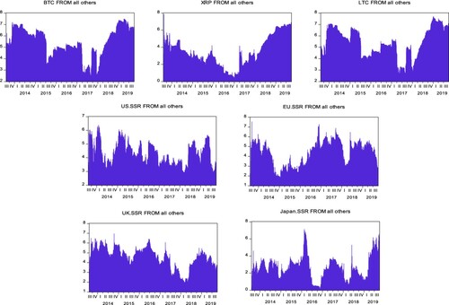
Figure 4 plots the time-varying net directional spillovers from each underlying variable to all other variables. It shows that net spillovers from Bitcoin and Litecoin have generally been positive, while those for Ripple have been negative. Thus, while Bitcoin and Litecoin are net transmitters of shocks, Ripple appears to be a net receiver even though net (negative) spillovers have been narrowing over time.

Figure 4. Dynamic net directional spillover indices.

Notes: This Figure displays the time-varying behaviour of the net directional spillovers from each underlying variable to all other variables. Positive (negative) values indicate that the variable under consideration is a net transmitter (receiver) of spillovers to (from) all other variables. Spillovers are based on the generalised forecast-error variance decomposition (GFEVD) obtained from the estimation of a TVP-VAR model of order 2 and 10-step ahead forecasts. The sample period is August 5, 2013 – September 27, 2019. The lag length is selected in accordance with the Bayesian information criterion (BIC).

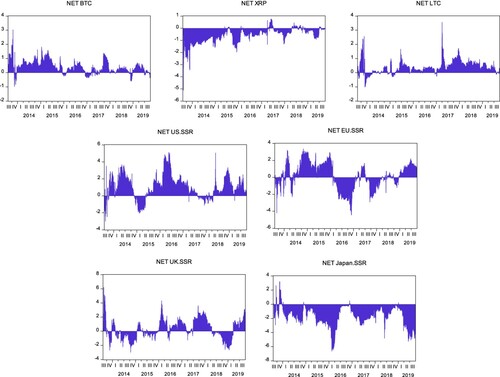
Regarding international monetary policy, the empirical evidence suggests that: (i) the US is typically a net transmitter of shocks; (ii) there are periods in which the Eurozone and the UK are net transmitters of shocks and others where they are net receivers of shocks; and (iii) Japan is generally a net receiver of shocks. Given that monetary policy has not been synchronised over the past years as a reflex of a different positioning of the economies under consideration in the business cycle, these results are indicative of the measures put forward by central banks at specific points in time (i.e. around announcements) and the subsequent international monetary spillovers (Avdjiev et al., 2020). Thus, when a given monetary authority adopted a set of policy measures, it became a net transmitter of shocks, with other economies becoming a net receiver of shocks. Additionally, the ongoing sovereign debt crisis in the Eurozone in the first half of the sample period might help to explain why it was a key source of net monetary spillovers. As for the more recent period, it appears to largely influenced by the Brexit referendum, which made the UK responsible for the largest net directional spillovers.

Finally, in Figure 5, we apply network analysis to plot the net pairwise spillovers. Specifically, the Figure portrays the average pairwise directional spillovers, where a node’s colour identifies if a variable is a net transmitter (receiver) of shocks to (from) other variables. In particular, the red colour indicates that the variable is a net transmitter of spillovers, while the green colour denotes the case in which the variable is a net receiver of spillovers. Furthermore, the thickness and the colour of the arrows represent the magnitude and strength of the average spillover from one node to another, respectively. In this case, the navy colour indicates strong spillovers, the blue colour shows moderate spillovers, and the light blue colour refers to weak spillovers.

Figure 5. Network of directional pairwise spillovers.

Notes: This Figure portrays the net directional pairwise spillovers among all possible pairs of variables. A node’s colour identifies if a variable is a net transmitter/receiver of shocks to/from other variables. The red (green) colour indicates that the variable is a net transmitter (receiver) of spillovers. Furthermore, the thickness and the colour of the arrows represent the magnitude and strength of the average spillover between each pair, respectively. In this case, the navy colour of the arrows indicates strong spillovers, the blue colour shows moderate spillovers, and the light blue colour refers to weak spillovers. Spillovers are based on the generalised forecast-error variance decomposition (GFEVD) obtained from the estimation of a TVP-VAR model of order 2 and 10-step ahead forecasts. The sample period is August 5, 2013 – September 27, 2019. The lag length is selected in accordance with the Bayesian information criterion (BIC).

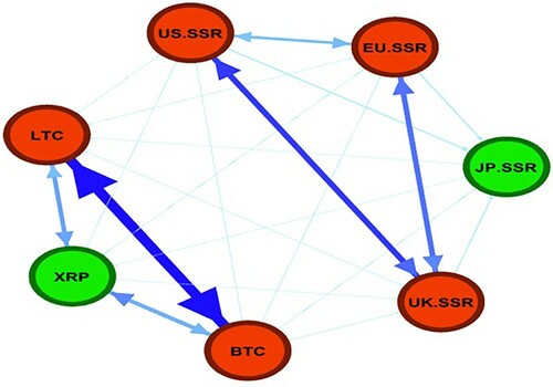
The Figure shows that there is strong interconnectedness among cryptocurrency returns. In particular, the net directional pairwise spillovers between Bitcoin and Litecoin are strong. This finding is close in spirit with the study of Corbet et al. (2018), who also highlight that cryptocurrencies are strongly interconnected and can be seen as a new investment class. Additionally, while both Bitcoin and Litecoin are net transmitters of shocks, Ripple is a net receiver of shocks. Regarding the net directional pairwise spillovers between monetary policy, we find that they are especially strong between the US and the UK. They are also moderate between the US and the Eurozone and between the UK and the Eurozone. Moreover, the shadow policy rates of these three economies are net transmitters of shocks, while Japan is a net receiver of shocks. This corroborates the finding of Antonakakis et al. (2019) about the dominant role of the US and the Eurozone as transmitters of monetary policy spillovers. Finally, the empirical evidence suggests that the spillovers between international monetary policy and cryptocurrency returns are, overall, weak.

4.3 Conventional versus unconventional monetary policy

In this Section, we investigate if the transmission of monetary policy spillovers differs between periods of US conventional monetary policy and unconventional monetary policy (i.e. the zero lower bound). Thus, to assess the importance of this feature, we analyse the spillovers between monetary policy and cryptocurrency markets in two distinct periods. The first (i.e. August 5, 2013 – December 16, 2015) captures the period over which unconventional monetary policy has been in place. The second (i.e. December 17, 2015 – September 27, 2019). This split of the sample is in accordance with the procedure followed by Antonakakis et al. (2019) and Corbet et al. (2020), and largely overlap with the periods over which the US shadow policy rate was either negative or positive. From an empirical perspective, the emphasis in the US monetary policy is also supported by the works of Georgiadis (2016) and Georgiadis and Mehl (2016), who highlight its role as a source of global risk appetite and international financial spillovers. Additionally, several papers analyse the international spillovers from US monetary policy (Avdjiev and Hale, 2019; Hoek et al., 2020; Avdjiev et al., 2020).

Table 3 summarises the findings for the period of US unconventional monetary policy, while Table 4 provides the results for the US conventional monetary era. Overall, the total connectedness index (TCI) was only slightly larger during the zero lower bound period compared to the period of normalisation of monetary policy (28.8% and 25.5%, respectively). Cook and Devereux (2016) also show that unconventional monetary policy spillovers tend to be larger than those associated with monetary policy in ‘normal times’. Our result is in line with the finding of Antonakakis et al. (2019), who point out that monetary policy spillovers did not significantly change between unconventional and conventional eras.

Table 3. Connectedness – Unconventional monetary policy (August 5, 2013 – December 16, 2015).

	BTC	XRP	LTC	US.SSR	EU.SSR	JP.SSR	UK.SSR	FROM others
BTC	58.31	8.87	31.57	0.47	0.21	0.41	0.16	41.69
XRP	12.26	78.21	7.94	0.38	0.72	0.01	0.48	21.79
LTC	31.91	7.42	59.05	0.31	0.62	0.35	0.35	40.95
US.SSR	0.04	0.30	0.09	69.15	9.92	0.61	19.91	30.85
EU.SSR	0.18	0.53	0.28	8.86	81.26	0.05	8.85	18.74
JP.SSR	1.11	0.22	0.11	4.76	6.94	85.98	0.87	14.02
UK.SSR	0.51	0.06	0.18	19.05	13.16	0.23	66.81	33.19
TO others	46.01	17.38	40.15	33.83	31.57	1.66	30.61	201.23
Net spillovers	4.33	−4.41	−0.80	2.98	12.83	−12.36	−2.58	TCI = 28.75%

Notes: This Table summarises the empirical results of the total, directional and pairwise spillovers. They are based on the generalised forecast-error variance decomposition (GFEVD) obtained from the estimation of a TVP-VAR model of order 2 and 10-step ahead forecasts. The sample period is August 5, 2013 – December 16, 2015. The lag length is selected in accordance with the Bayesian information criterion (BIC). ‘TO' directional spillovers correspond to the off-diagonal column sums (labelled contributions TO others), i.e. spillovers from variable i to all variables j. 'FROM' directional spillovers denote the off-diagonal row sums (labelled contributions FROM others), i.e. spillovers from all variables j to variable i. Net spillovers ('NET') are simply the "from" minus "to" differences. The total spillover index, which appears in the lower right corner of the Table, is approximately the grand off-diagonal column sum (or row sum) relative to the grand column sum including the diagonals (or row sum including diagonals), expressed as a percentage.

Table 4. Connectedness – Conventional monetary policy (December 17, 2015 – September 27, 2019).

	BTC	XRP	LTC	US.SSR	EU.SSR	JP.SSR	UK.SSR	FROM others
BTC	66.55	9.98	22.96	0.08	0.07	0.29	0.08	33.45
XRP	10.40	75.16	13.92	0.08	0.07	0.20	0.17	24.84
LTC	22.49	10.95	65.87	0.12	0.19	0.15	0.23	34.14
US.SSR	0.16	0.15	0.21	78.98	8.07	0.42	12.01	21.02
EU.SSR	0.12	0.00	0.10	13.73	68.87	0.76	16.43	31.13
JP.SSR	0.05	0.06	0.19	3.62	6.45	86.81	2.82	13.19
UK.SSR	0.24	0.11	0.25	9.72	9.89	0.22	79.57	20.43
TO others	33.45	21.26	37.62	27.34	24.74	2.04	31.75	178.19
Net spillovers	0.00	−3.58	3.48	6.32	−6.40	−11.14	11.32	TCI = 25.46%

Notes: This Table summarises the empirical results of the total, directional and pairwise spillovers. They are based on the generalised forecast-error variance decomposition (GFEVD) obtained from the estimation of a TVP-VAR model of order 2 and 10-step ahead forecasts. The sample period is December 17, 2015 – September 27, 2019. The lag length is selected in accordance with the Bayesian information criterion (BIC). ‘TO' directional spillovers correspond to the off-diagonal column sums (labelled contributions TO others), i.e. spillovers from variable i to all variables j. 'FROM' directional spillovers denote the off-diagonal row sums (labelled contributions FROM others), i.e. spillovers from all variables j to variable i. Net spillovers ('NET') are simply the "from" minus "to" differences. The total spillover index, which appears in the lower right corner of the Table, is approximately the grand off-diagonal column sum (or row sum) relative to the grand column sum including the diagonals (or row sum including diagonals), expressed as a percentage.

During the period of unconventional monetary policy and among shadow short-rates, the largest gross directional spillovers to others were generated by the US (33.8%), being followed by the Eurozone (31.6%) and the UK (30.6%). By contrast, gross directional spillovers from the shadow short-rate of Japan to others are negligible (1.7%). As for cryptocurrency returns, the largest gross directional spillovers to others are attributed to Bitcoin (46%), followed by Litecoin (40.2%).

As for the period of conventional monetary policy, directional spillovers to others were lower for the US and the Eurozone and slightly larger for the UK and Japan. Regarding cryptocurrency returns, the gross directional spilovers were generally lower, ranging between 21.3% (Ripple) and 37.6% (Litecoin). These results are in line with those reported by Corbet et al. (2020), who find smaller volatility spillovers among cryptocurrencies in the second period compared to the first period, as markets become more mature.

Looking at the ‘‘directional from others’’ column, we find that: (i) among shadow policy rates, the largest gross directional spillovers from others were observed in the US (30.9%) and the UK (33.2%) during unconventional monetary policy and in the Eurozone (31.1%) during conventional monetary policy; and (ii) among cryptocurrency returns, the gross directional spillovers from others were larger for Bitcoin and Litecoin during unconventional monetary policy (i.e. 41.7% and 41%, respectively) than during conventional monetary policy (33.5% and 34.1%, respectively), For Ripple, the opposite was detected.

As for the net directional spillovers, they are positive for the US and negative for Ripple and Japan in both periods. However, they shifted from positive to negative in the case of the Eurozone, and from negative to positive in the case of the UK, again suggesting the role played by the Eurozone sovereign debt crisis in the first half of the sample and the outcome of the Brexit referendum in the second half of the sample period. In this context, Antonakakis et al. (2019) find that the US was a dominant transmitter (receiver) of shocks during the unconventional (conventional) US monetary policy era. Interestingly, net spillovers were roughly nil for Litecoin in the first sub-sample period (i.e. US unconventional monetary policy) and for Bitcoin in the second sub-sample period (i.e. US conventional monetary policy).

Finally, in Figure 6, we apply network analysis to plot the net pairwise spillovers computed for the two sub-sample periods. The left panel denotes the period of non-standard monetary policy, while the right panel corresponds to the period of standard monetary policy. It can be seen that interconnectedness among cryptocurrency returns (in particular, between Bitcoin and Litecoin) remains strong across the two periods. However, while Litecoin was a net receiver of shocks when unconventional monetary policy was in place, it became a net transmitter of shocks afterwards. Moreover, Bitcoin was a net transmitter of volatility spillovers during the first period, but became neutral in the second period (as indicated by the node’s light brown colour). These results are in line with those of Bouoiyour and Selmi (2016), who note that Bitcoin’s volatility rapidly declined over time. Hence, it is less likely to transmit shocks to other markets as a result of becoming a more mature crypto market.

Figure 6. Network of directional pairwise spillovers – Conventional versus unconventional monetary policy.

Notes: Panels A and B portray the net directional pairwise spillovers among all possible pairs of variables. A node’s colour identifies if a variable is a net transmitter/receiver of shocks to/from other variables. The red (green) colour indicates that the variable is a net transmitter (receiver) of spillovers, while the light brown colour indicates that the variable is neutral. Furthermore, the thickness and the colour of the arrows represent the magnitude and strength of the average spillover between each pair, respectively. In this case, the navy colour of the arrows indicates strong spillovers, the blue colour shows moderate spillovers, and the light blue colour refers to weak spillovers. Spillovers are based on the generalised forecast-error variance decomposition (GFEVD) obtained from the estimation of a TVP-VAR model of order 2 and 10-step ahead forecasts. The sub-sample periods are August 5, 2013 – December 16, 2015 and December 17, 2015 – September 27, 2019. The lag length is selected in accordance with the Bayesian information criterion (BIC).

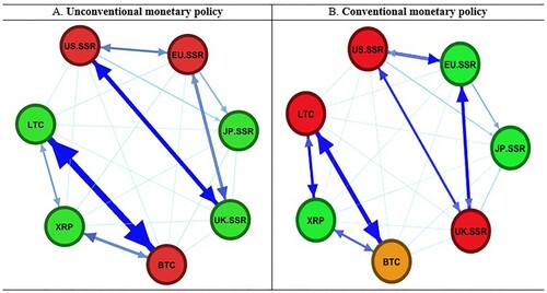
Regarding the net directional pairwise spillovers between monetary policy, we find that they are especially strong between the US and the UK, and somewhat moderate between the US and the Eurozone and between the UK and the Eurozone. The key difference between the two sub-sample periods is that the Eurozone (UK) is a net transmitter (receiver) of shocks during unconventional (conventional) monetary policy. Overall, the net pairwise spillovers between international monetary policy and cryptocurrency returns are weak across the two sub-sample periods.

5. Conclusion

We investigate the time-varying nature of interconnectedness between international monetary policy spillovers, cryptocurrency spillovers and spillovers across monetary policy and cryptocurrency markets using data for shadow policy rates of four major economies (Eurozone, Japan, UK and US) and three large cryptocurrencies (Bitcoin, Litecoin and Ripple) over the period August 5, 2013 – September 27, 2019.

To do so, we employ the Time-Varying Parameter Vector Auto-Regression (TVP-VAR) model developed by Koop and Korobilis (2014) in conjunction with the dynamic connectedness approach by Diebold and Yilmaz (2009, 2012, 2014). We also apply the network analysis developed by Jacomy et al. (2014) to illustrate the interconnectedness between the variables included in the model.

Our framework reveals not only a relatively large degree of interconnectedness, but also one that is time-varying in nature. Specifically, cryptocurrency returns and monetary policy spillovers were particularly large when central banks put forward large-scale non-standard monetary policies and shadow policy rates became negative. Then, they started to diminish as the Fed's ‘tapering process’ was initiated, despite some occasional spikes surrounding monetary policy announcements. Finally, spillovers rose again more recently, as shadow policy rates in the US and the Eurozone fell and cryptocurrency buoyancy returned.

Additionally, while gross directional spillovers of shadow policy rates from all others typically suggest that they have more ‘to give than to receive’, those from and to cryptocurrency returns embed occasional spikes just like their own intrinsic volatility.

The empirical evidence also supports the view of a somewhat low monetary policy synchronisation in recent years, as economic growth geared at different speeds across jurisdictions. Thus, the US (Japan) is generally a net transmitter (receiver) of shocks, while the Eurozone and the UK are both net transmitters and receivers. As for cryptocurrencies, Bitcoin and Litecoin are net transmitters of shocks, while Ripple is a net receiver.

Our network analysis also reveals strong interconnected between monetary policy in either the US or the Eurozone and the UK, and between Bitcoin and Litecoin. However, the spillovers across monetary policy and cryptocurrencies tend to be muted.

Finally, spillovers appear to be only slightly quantitatively larger during the Fed's ‘non-standard’ monetary policy compared to ‘normal’ periods. Yet, their composition appears to have changed qualitatively over time. Specifically, net directional spillovers: (i) shifted from positive (negative) to negative (positive) in the Eurozone (UK); and (ii) are nil for Litecoin (Bitcoin) during US unconventional (conventional) monetary policy.

From a policy perspective, our findings of strong international monetary spillovers pose challenges for national authorities, reinforcing the importance of policy coordination. In particular, setting up a global level playing field might be relevant to avoid regulatory arbitrage and deter any potential financial instability that might be attributed to sharp shifts in capital flows associated with portfolio reallocations into and away from the cryptocurrency space. From a practitioner's view, as cryptocurrency returns appear to be immune to such spillovers, they might offer diversification benefits from speculative positions in digital assets (Bouoiyour and Selmi, 2015; Bouoiyour et al., 2016; Selmi et al., 2018). Specifically, portfolio managers in interest rate-sensitive financial instruments (e.g. derivatives) might improve their returns by using cryptocurrencies as a hedge against the risk embedded in monetary policy actions. Speculative investors could also mitigate risk through the diversification of their portfolios by adding cryptocurrencies to interest rate derivatives.

Our work paves the way for new avenues of research. First, a promising direction to explore consists on investigating the spillovers between cryptocurrency returns and micro- and macro-prudential policies, as well as the exploitation of regulatory arbitrage across cryptocurrency markets. Second, we also plan to assess such interconnectedness not only with the use of time-domain, but also frequency-domain spillover methods. This should enlighten how the dynamic linkages between cryptocurrency returns and economic policy evolve at different business cycle frequencies. We leave this investigation for the future.

Acknowledgments

The authors would like to thank Larisa Yarovaya, Andrew Urquhart, Shaen Corbet, and seminar participants at the Cryptocurrency Research Conference 2020 for their constructive comments and suggestions.

Disclosure statement

No potential conflict of interest was reported by the author(s).

Additional information

Funding

This work was supported by National Funds of the FCT – Portuguese Foundation for Science and Technology [Grant Number UIDB/ECO/03182/2020].

Notes on contributors

Ahmed H. Elsayed

Dr. Ahmed H. Elsayed is an Associate Professor in Economics and Finance at Durham University. He is also a Research Fellow of the SDGs Network, the Economic Research Forum, and the Institute for Middle Eastern and Islamic Studies, among many other institutions. Dr. Elsayed is acting as an Associate Editor of Heliyon Business and Economics and has published in top prestigious Economics and Finance journals such as Economics Letters, European Journal of Finance, International Review of Financial Analysis, Journal of International Financial Markets, Institutions and Money, Energy Economics, Annals of Operation Research, and International Journal of Finance and Economics, among others.

Ricardo M. Sousa

Ricardo M. Sousa is an Associate Professor with Habilitation at the Department of Economics, a Researcher at the Economic Policies Research Unit (NIPE) of the University of Minho, and an Associate Editor of the Economic Modelling. Previously, he worked as a Senior Economist at the Bank for International Settlements (BIS) and the European Stability Mechanism (ESM), as an Economist at the Bank of England (BoE) and the European Central Bank (ECB), and held visiting positions at the Bank of Portugal and the International Monetary Fund (IMF).

Notes

1 As a robustness check of the sensitivity of the model against outliers and asymmetry, we also compute spillovers using a Quantile VAR model (QVAR). In this framework, the estimated spillover index overcomes the outlier sensitivity problem of the VAR model and captures potential asymmetry, as it is calculated based on the conditional median rather than the conditional mean. Our findings show that the spillover index based on the TVP-VAR model strongly co-move with the spillover indices estimated from a rolling window Quantile Vector Autoregressive model (RW-QVAR) and a rolling window Vector Autoregressive model (RW-VAR). However, the TVP-VAR spillover index adjusts faster to market conditions than its counterparts. This empirical advantage has previously been discussed and stressed by Korobilis and Yilmaz (2018) and Antonakakis et al. (2020). For brevity, these results are not reported in the paper, but they are available from the authors upon request.

2 In this context, the TVP-VAR approach has been widely used in the literature to assess connectedness and spillovers (Antonakakis and Gabauer, 2017; Korobilis and Yilmaz, 2018; Bouri et al., 2021).

3 Following the related literature, we have estimated variance decomposition functions based on 10-step-ahead forecasts (Diebold and Yılmaz, 2012; Antonakakis and Gabauer, 2017; Korobilis and Yilmaz, 2018; Antonakakis et al., 2019; Bouri et al., 2021). Despite this and to assess the sensitivity of the empirical findings to the choice of the forecast horizons, we have also considered different forecast horizons (namely, H = 15, H = 20 and H = 30 days). The empirical findings are very similar to those reported in the paper and they are available from the authors upon request.

4 Cryptocurrency price data are obtained from: http://www.coinmarketcap.com.

5 Shadow short-rates can be downloaded at: https://www.rbnz.govt.nz/research-and-publications/research-programme/additional-research/measures-of-the-stance-of-united-states-monetary-policy/comparison-of-international-monetary-policy-measures.

6 While ‘too much’ data can obviously lead to model overfitting and wrong predictions, large amounts of data ease the classification of outliers and improve the clarity about the underlying distribution of such data, thus, improving the power of the TVP-VAR model vis-à-vis a fixed-coefficient VAR model (Koop and Korobilis, 2014). The importance of high-frequency data for the accuracy of the empirical findings is well-portrayed by the computational tractability requirements associated with the use of low-frequency data. More specifically, our study uses more than 2200 daily data points, which compares to a mere 74 monthly data points. Not surprisingly,

despite delivering quantitatively different, but qualitatively similar, gross directional spillovers, the estimation of the TVP-VAR model using monthly data generates several qualitative and quantitative incongruencies. These are available from the authors upon request. Thus, not only is the consideration of the TVP-VAR model relevant, also the data frequency matters in obtaining more accurate and reliable estimates of the dynamic connectedness between international monetary policies and cryptocurrency returns. Indeed, investors and fund managers adjust their portfolios very quickly in respond to monetary policy changes, hence, daily data are more appropriate in capturing such immediate response. For example, Nakamura and Steinsson (2018a, 2018b) stress the importance of high-frequency data to obtain more clarity about the monetary policy dynamics. Furthermore, Antonakakis et al. (2019) point out that knowledge of monetary policy spillovers at a high-frequency is more beneficial to investors and policy makers in determining the direction that the economy is heading to in the future. Consequently, the use of monthly data ‘masks’ important information about the dynamic connectedness and response of cryptocurrency returns to monetary policy changes.

 

 

7 While the outperformance of the TVP-VAR model vis-à-vis the fixed-coefficient VAR model and the sensitivity of the latter to the presence of outliers are confirmed by the application of Monte Carlo simulations, the robustness to the rolling window size and the avoidance of information loss by the former are self-evident by construction. Moreover, the use of a time-varying variance-covariance structure allows us to accurately model structural changes in the underlying system. Despite this, we also estimate a fixed-coefficients VAR model for the full sample period. While qualitatively similar, we find that the Total Connectedness Index (TCI), the gross directional spillovers ‘TO’ others and ‘FROM’ others and the net direction spillovers are larger in the fixed-coefficients VAR model compared to the TVP-VAR model reported in Table 2. Thus, the consideration of the TVP-VAR model is relevant in this regard. For brevity, these results are not reported in the paper, but they are available from the authors upon request.

References

- Agnello, L., V. Castro, G. Dufrénot, F. Jawadi, and R. M. Sousa. 2019. “Unconventional Monetary Policy Reaction Functions: Evidence from the US.” Studies in Nonlinear Dynamics and Econometrics 24 (4): 20180088.
- Antonakakis, N., I. Chatziantoniou, and D. Gabauer. 2020. “Refined Measures of Dynamic Connectedness Based on Time-Varying Parameter Vector Autoregressions.” Journal of Risk and Financial Management 13 (4): 84–106.
- Antonakakis, N., and D. Gabauer. 2017. Refined measures of dynamic connectedness based on TVP-VAR. University Library of Munich, MPRA Paper no. 78282.
- Antonakakis, N., D. Gabauer, and R. Gupta. 2019. “International Monetary Policy Spillovers: Evidence from a Time-Varying Parameter Vector Autoregression.” International Review of Financial Analysis 65: 101382.
- Antonakakis, N., D. Gabauer, R. Gupta, and V. Plakandaras. 2018. “Dynamic Connectedness of Uncertainty Across Developed Economies: A Time-Varying Approach.” Economics Letters 166: 63–75.
- Auer, R. 2019. Beyond the doomsday economics of “proof-of-work” in cryptocurrencies. Bank for International Settlements, BIS Working Paper no. 765.
- Auer, R., and S. Claessens. 2018. Regulating cryptocurrencies: assessing market reactions. BIS Quarterly Review, September, 51–65.
- Avdjiev, S., L. Gambacorta, L. Goldberg, and S. Schiaffi. 2020. “The Shifting Drivers of Global Liquidity.” Journal of International Economics 125: 103324.
- Avdjiev, S., and G. Hale. 2019. “US Monetary Policy and Fluctuations of International Bank Lending.” Journal of International Money and Finance 95: 251–268.
- Banerjee, A., M. Marcellino, and I. Masten. 2008. Forecasting macroeconomic variables using diffusion indexes in short samples with structural change. Frontiers of Economics and Globalization, Forecasting in the Presence of Structural Breaks and Model Uncertainty: Volume 3, Chapter 4, 149–194.
- Bariviera, A. F., M. J. Basgall, W. Hasperué, and M. Naiouf. 2017. “Some Stylized Facts of the Bitcoin Market.” Physica A: Statistical Mechanics and its Applications 484: 82–90.
- Bates, B. J., M. Plagborg-Møller, J. H. Stock, and M. W. Watson. 2013. “Consistent Factor Estimation in Dynamic Factor Models with Structural Instability.” Journal of Econometrics 177: 289–304.
- Baur, D. G., K. Hong, and A. D. Lee. 2018. “Bitcoin: Medium of Exchange or Speculative Assets?” Journal of International Financial Markets, Institutions & Money 54: 177–189.
- Belke, A., and I. Dubova. 2018. “International Spillovers in Global Asset Markets.” Economic Systems 42 (1): 3–17.
- Belke, A., I. Dubova, and U. Volz. 2018. “Bond Yield Spillovers from Major Advanced Economies to Emerging Asia.” Pacific Economic Review 23 (1): 109–126.
- Bernanke, B. S., and V. R. Reinhart. 2004. “Conducting Monetary Policy at Very low Short-Term Interest Rates.” American Economic Review 94 (2): 85–90.
- Blinder, A. 2000. “Monetary Policy at the Zero Lower Bound: Balancing the Risks.” Journal of Money, Credit and Banking 32 (4): 1093–1099.
- Blundell, R., and S. Bond. 1998. “Initial Conditions and Moment Restrictions in Dynamic Panel Data Models.” Journal of Econometrics 87 (1): 115–143.
- Bouoiyour, J., and R. Selmi. 2015. “What Does Bitcoin Look Like?” Annals of Economics and Finance 16 (2): 449–492.
- Bouoiyour, J., and R. Selmi. 2016. “Bitcoin: A Beginning of a new Phase?” Economics Bulletin 36 (3): 1430–1440.
- Bouoiyour, J., R. Selmi, and A. K. Tiwari. 2015. “Is Bitcoin Business Income or Speculative Foolery? New Ideas Through an Improved Frequency Domain Analysis.” Annals of Financial Economics 10 (1): 1–23.
- Bouoiyour, J., R. Selmi, A. K. Tiwari, and O. R. Olayeni. 2016. “What Drives Bitcoin Price?” Economics Bulletin 36 (2): 843–850.
- Bouoiyour, J., R. Selmi, and M. E. Wohar. 2019. “Bitcoin: Competitor or Complement to Gold?” Economics Bulletin 39 (1): 186–191.
- Bouri, E., O. Cepni, D. Gabauer, and R. Gupta. 2021. “Return Connectedness Across Asset Classes Around the COVID-19 Outbreak.” International Review of Financial Analysis 73: 101646.
- Bouri, E., P. Molnár, G. Azzi, D. Roubaud, and L. I. Hagfors. 2017. “On the Hedge and Safe Haven Properties of Bitcoin: Is it Really More Than a Diversifier?” Finance Research Letters 20: 192–198.
- Böhme, R., N. Christin, B. Edelman, and T. Moore. 2015. “Bitcoin: Economics, Technology, and Governance.” Journal of Economic Perspectives 29 (2): 213–238.
- Brandvold, M., P. Molnár, K. Vagstad, and O. C. Andreas Valstad. 2015. “Price Discovery on Bitcoin Exchanges.” Journal of International Financial Markets, Institutions & Money 36: 18–35.
- Breitung, J., and S. Eickmeier. 2011. “Testing for Structural Breaks in Dynamic Factor Models.” Journal of Econometrics 163 (1): 71–84.
- Buffett, W. 2018. Probably rat poison squared. Berkshire Hathaway's annual shareholder meeting. Omaha, Nebraska, USA, 6 May.
- Carstens, A. 2017. A combination of bubble, a Ponzi scheme and an environmental disaster. G30 International Banking seminar, Washington, DC, USA, 15 October.
- Cheah, E. T., and J. Fry. 2015. “Speculative Bubbles in Bitcoin Markets? An Empirical Investigation Into the Fundamental Value of Bitcoin.” Economics Letters 130: 32–36.
- Chen, Q., A. Filardo, D. He, and F. Zhu. 2016. “Financial Crisis, US Unconventional Monetary Policy and International Spillovers.” Journal of International Money and Finance 67: 62–81.
- Christensen, J., and G. D. Rudebusch. 2016. “Modeling Yields at the Zero Lower Bound: Are Shadow Rates the Solution?” In Dynamic Factor Models, Advances in Econometrics, 35, edited by E. Hillebrand, and S. J. Koopman, 75–125. Bingley: Emerald Group Publishing Limited.
- Claessens, S., L. Stracca, and F. E. Warnock. 2016. “International Dimensions of Conventional and Unconventional Monetary Policy.” Journal of International Money and Finance 67: 1–7.
- Claus, E., I. Claus, and L. Krippner. 2016. “Monetary Policy Spillovers Across the Pacific When Interest Rates are at the Zero Lower Bound.” Asian Economic Papers 15 (3): 1–27.
- Constâncio, V. 2017. Bitcoin is a sort of tulip. ECB conference, Frankfurt, Germany, 22 September.
- Cook, D., and M. B. Devereux. 2016. “Exchange Rate Flexibility Under the Zero Lower Bound.” Journal of International Economics 101 (C): 52–69.
- Corbet, S., C. Larkin, B. Lucey, A. Meegan, and L. Yarovaya. 2020. “Cryptocurrency Reaction to FOMC Announcements: Evidence of Heterogeneity Based on Blockchain Stack Position.” Journal of Financial Stability 46: 100706.
- Corbet, S., B. Lucey, A. Urquhart, and L. Yarovaya. 2019. “Cryptocurrencies as a Financial Asset: A Systematic Analysis.” International Review of Financial Analysis 62: 182–199.
- Corbet, S., A. Meegan, C. Larkin, B. Lucey, and L. Yarovaya. 2018. “Exploring the Dynamic Relationships Between Cryptocurrencies and Other Financial Assets.” Economics Letters 165: 28–34.
- Demir, E., G. Gozgor, C. K. M. Lau, and S. A. Vigne. 2018. “Does Economic Policy Uncertainty Predict the Bitcoin Returns?” An Empirical Investigation. Finance Research Letters 26: 145–149.
- Diebold, F. X., and K. Yilmaz. 2009. “Measuring Financial Asset Return and Volatility Spillovers, with Application to Global Equity Markets.” Economic Journal 119: 158–171.
- Diebold, F. X., and K. Yilmaz. 2012. “Better to Give Than to Receive: Predictive Directional Measurement of Volatility Spillovers.” International Journal of Forecasting 28: 57–66.
- Diebold, F. X., and K. Yilmaz. 2014. “On the Network Topology of Variance Decompositions: Measuring the Connectedness of Financial Firms.” Journal of Econometrics 182: 119–134.
- Dimon, J. 2017. It’s just not a real thing, eventually it will be closed. Delivering Alpha conference, New York, USA, 12 September.
- Dwyer, G. P. 2015. “The Economics of Bitcoin and Similar Private Digital Currencies.” Journal of Financial Stability 17: 81–91.
- Dyhrberg, A. H., S. Foley, and J. Svec. 2018. “How Investible is Bitcoin? Analyzing the Liquidity and Transaction Costs of Bitcoin Markets.” Economics Letters 171: 140–143.
- Eichengreen, B. 2015. “Secular Stagnation: The Long View.” American Economic Review 105: 66–70.
- Fry, J. 2018. “Booms, Busts and Heavy-Tails: The Story of Bitcoin and Cryptocurrency Markets?” Economics Letters 171: 225–229.
- Gabauer, D., and R. Gupta. 2018. “On the Transmission Mechanism of Country-Specific and International Economic Uncertainty Spillovers: Evidence from a TVP-VAR Connectedness Decomposition Approach.” Economics Letters 171: 63–71.
- Galariotis, E., P. Makrichoriti, and S. Spyrou. 2018. “The Impact of Conventional and Unconventional Monetary Policy on Expectations and Sentiment.” Journal of Banking & Finance 86: 1–20.
- Gandal, N., J. Hamrick, T. Moore, and T. Oberman. 2018. “Price Manipulation in the Bitcoin Ecosystem.” Journal of Monetary Economics 95: 86–96.
- Georgiadis, G. 2016. “Determinants of Global Spillovers from US Monetary Policy.” Journal of International Money and Finance 67: 41–61.
- Georgiadis, G., and A. Mehl. 2016. “Financial Globalisation and Monetary Policy Effectiveness.” Journal of International Economics 103: 200–212.
- Greenspan, A. 2013. It's a bubble. Bloomberg Television, interview, 4 December.
- Guesmi, K., S. Saadi, I. Abid, and Z. Ftiti. 2019. “Portfolio Diversification with Virtual Currency: Evidence from Bitcoin.” International Review of Financial Analysis 63: 431–437.
- Hall, R. 2016. Understanding the decline in the safe real interest rate. Stanford University, Manuscript.
- Hatemi-J, A., M. A. Hajji, E. Bouri, and R. Gupta. 2021. “The Benefits of Diversification Between Bitcoin, Bonds, Equities and the US Dollar: A Matter of Portfolio Construction.” Asia-Pacific Journal of Operational Research, doi:https://doi.org/10.1142/S0217595920400242.
- Hoek, J., S. Kamin, and E. Yoldas. 2020. When is bad news good news? US monetary policy, macroeconomic news, and financial conditions in emerging markets. Board of Governors of the Federal Reserve System, International Finance Discussion Paper no. 1269.
- Jacomy, M., T. Venturini, S. Heymann, and M. Bastian. 2014. “ForceAtlas2, a Continuous Graph Layout Algorithm for Handy Network Visualization Designed for the Gephi Software.” PloS one 9: e98679.
- Jawadi, F., R. M. Sousa, and R. Traverso. 2017. “On the Macroeconomic and the Wealth Effects of Unconventional Monetary Policy.” Macroeconomic Dynamics 21 (5): 1189–1204.
- Ji, Q., E. Bouri, R. Gupta, and D. Roubaund. 2018. “Network Causality Structures among Bitcoin and Other Financial Assets: A Directed Acyclic Graph Approach.” Quarterly Review of Economics and Finance 70: 203–213.
- Klein, T., H. P. Thu, and T. Walther. 2018. “Bitcoin is not the New Gold - a Comparison of Volatility, Correlation, and Portfolio Performance.” International Review of Financial Analysis 59: 105–116.
- Koop, G., and D. Korobilis. 2014. “A new Index of Financial Conditions.” European Economic Review 71: 101–116.
- Koop, G., M. H. Pesaran, and S. M. Potter. 1996. “Impulse Response Analysis in Nonlinear Multivariate Models.” Journal of Econometrics 74: 119–147.
- Korobilis, D., and K. Yilmaz. 2018. Measuring dynamic connectedness with large Bayesian VAR models. Koç University-TUSIAD Economic Research Forum, Working Paper no. 1802.
- Krippner, L. 2013. “Measuring the Stance of Monetary Policy in Zero Lower Bound Environments.” Economics Letters 118 (1): 135–138.
- Krippner, L. 2015. A comment on Wu and Xia (2015), and the case for two-factor shadow short rates. Australian National University, Crawford School of Public Policy, Centre for Applied Macroeconomic Analysis, CAMA Working Paper no. 48.
- Kristoufek, L. 2015. “What are the Main Drivers of the Bitcoin Price? Evidence from Wavelet Coherence Analysis.” PloS one 10 (4): e0123923.
- Krugman, P. 2018. Bubble, bubble, fraud and trouble. The New York Times, 29 January.
- Kyriazis, N. A. 2019. “A Survey on Empirical Findings About Spillovers in Cryptocurrency Markets.” Journal of Risk and Financial Management 12 (4): 170.
- Li, X., and C. A. Wang. 2017. “The Technology and Economic Determinants of Cryptocurrency Exchange Rates: The Case of Bitcoin.” Decision Support Systems 95: 49–60.
- Liu, L., C. Matthes, and K. Petrova. 2018. Monetary policy across space and time. Federal Reserve Bank of Richmond, Working Paper no. 14.
- Lobo, B. J. 2000. “Asymmetric Effects of Interest Rate Changes on Stock Prices.” Financial Review 35: 125–144.
- Lombardi, M., and F. Zhu. 2014. A shadow policy rate to calibrate US monetary policy at the zero lower bound. Bank for International Settlements, BIS Working Paper no. 452.
- Ma, J. 2018. There's a bitcoin bubble. 2nd World Intelligence Congress, Tianjin, China, 16 May.
- Makarov, I., and A. Schoar. 2020. “Trading and Arbitrage in Cryptocurrency Markets.” Journal of Financial Economics 135 (2): 293–319.
- Mostak Ahamed, M., and S. K. Mallick. 2017a. “Does Regulatory Forbearance Matter for Financial Stability? Evidence from Creditors’ Perspective.” Journal of Financial Stability 28: 163–180.
- Mostak Ahamed, M., and S. K. Mallick. 2017b. “House of Restructured Assets: How do They Affect Bank Risk in an Emerging Market?” Journal of International Financial Markets, Institutions and Money 47: 1–14.
- Mostak Ahamed, M., and S. K. Mallick. 2019. “Is Financial Inclusion Good for Bank Stability? International Evidence.” Journal of Economic Behavior & Organization 157: 403–427.
- Nadarajah, S., and J. Chu. 2017. “On the Inefficiency of Bitcoin.” Economics Letters 150: 6–9.
- Nakamura, E., and J. Steinsson. 2018a. “High Frequency Identification of Monetary non-Neutrality: The Information Effect.” Quarterly Journal of Economics 133: 1283–1330.
- Nakamura, E., and J. Steinsson. 2018b. “Identification in Macroeconomics.” Journal of Economic Perspectives 32 (3): 59–86.
- Nguyen, T. V. H., B. T. Nguyen, K. S. Nguyen, and H. Pham. 2019. “Asymmetric Monetary Policy Effects on Cryptocurrency Markets.” Research in International Business and Finance 48: 335–339.
- Omane-Adjepong, M., and I. P. Alagidede. 2020. “Dynamic Linkages and Economic Role of Leading Cryptocurrencies in an Emerging Market.” Asia-Pacific Financial Markets 27: 537–585.
- Pesaran, H. H., and Y. Shin. 1998. “Generalized Impulse Response Analysis in Linear Multivariate Models.” Economics Letters 58: 17–29.
- Platanakis, E., and A. Urquhart. 2020. “Should Investors Include Bitcoin in Their Portfolios? A Portfolio Theory Approach.” The British Accounting Review 52 (4): 100837.
- Qarni, M. O., and S. Gulzar. 2021. “Portfolio Diversification Benefits of Alternative Currency Investment in Bitcoin and Foreign Exchange Markets.” Financial Innovation 7 (17): 1–37.
- Selmi, R., A. K. Tiwari, and S. Hammoudeh. 2018. “Efficiency or Speculation? A Dynamic Analysis of the Bitcoin Market.” Economics Bulletin 38 (4): 2037–2046.
- Sensoy, A. 2019. “The Inefficiency of Bitcoin Revisited: A High-Frequency Analysis with Alternative Currencies.” Finance Research Letters 28: 68–73.
- Shiller, R. 2014. In search of a stable electronic currency. The New York Times, 1 March.
- Soros, G. 2018. Cryptocurrencies are a bubble. World Economic Forum, Davos Switzerland, 25 January.
- Stiglitz, J. 2017. Bitcoin ‘ought to be outlawed’. Bloomberg Television, interview, 29 November.
- Stock, J., G. Elliott, and T. Rothenberg. 1996. “Efficient Tests for an Autoregressive Unit Root.” Econometrica 64 (4): 813–836.
- Summers, L. 2014. “U.S. Economic Prospects: Secular Stagnation, Hysteresis, and the Zero Lower Bound.” Business Economics 49: 65–73.
- Thaler, R. 2018. The market that looks most like a bubble to me is Bitcoin and its brethren. ECO Portuguese Economy, 22 January.
- Tillmann, P. 2016. “Unconventional Monetary Policy and the Spillovers to Emerging Markets.” Journal of International Money and Finance 66: 136–156.
- Tillmann, P., G.-Y. Kim, and H. Park. 2019. “The Spillover Effects of U.S. Monetary Policy on Emerging Market Economies.” International Journal of Finance and Economics 24 (3): 1313–1332.
- Turner, P. 2017. Did central banks cause the last financial crisis? Will they cause the next? LSE Financial Markets Group (FMG) Paper Series, Special Paper no. 249.
- Turner, P. 2018. “The Macroeconomics of Macroprudential Policies.” In Macroprudential Policy and Practice, Chapter 1, edited by P. Mizen, M. Rubio, and P. Turner, 19–45. Cambridge, UK: Cambridge University Press.
- Urquhart, A. 2017. “Price Clustering in Bitcoin.” Economics Letters 159: 145–148.
- Vidal-Tomas, D., and A. Ibañez. 2018. “Semi-strong Efficiency of Bitcoin.” Finance Research Letters 27: 259–265.
- Wu, J. C., and F. D. Xia. 2016. “Measuring the Macroeconomic Impact of Monetary Policy at the Zero-Lower Bound.” Journal of Money, Credit and Banking 48 (2-3): 253–291.
- Yelowitz, A., and M. Wilson. 2015. “Characteristics of Bitcoin Users: An Analysis of Google Search Data.” Applied Economics Letters 22 (13): 1030–1036.