Revealing the risk perception of investors using machine learning

Abstract

Corporate disclosures convey crucial information to financial market participants. While machine learning algorithms are commonly used to extract this information, they often overlook the use of idiosyncratic terminology and industry-specific vocabulary within documents. This study uses an unsupervised machine learning algorithm, the Structural Topic Model, to overcome these issues. Our findings illustrate the link between machine-extracted risk factors discussed in corporate disclosures (10-Ks) and the corresponding pricing behavior by investors, focusing on a previously unexplored US REIT sample from 2005 to 2019. Surprisingly, when disclosed, most risk factors counterintuitively lead to a decrease in return volatility. This resolution of uncertainties surrounding known risk factors or the provision of additional facts about these factors contributes valuable insights to the financial market.

KEYWORDS:

• Risk
• textual analysis
• machine learning
• structural topic model
• 10-K filing

JEL Classifications:

• C45
• C80
• G14
• G18
• M41
• R30

1. Introduction

It is still a matter of academic debate, whether markets efficiently incorporate information into prices. In financial markets, pricing is a continuous process of investors’ reactions to new information (Fama 1970) characterized by its volatility around the expected value. A low volatility is a sign of consistent expectations across investors regarding values when new information emerges. Contrary, high volatility indicates dissent about how to value and incorporate new information. By revealing a piece of new information, a new pricing process begins after their release date resulting in three possible outcomes: no price reaction if the information is irrelevant or already known among the investors, increasing volatility if the investors are in disagreement with the pricing outcome of the information, or decreasing volatility if the investors coincide about the informational impact on the firm’s future prospect. From a theoretical perspective, new information can increase or decrease investors’ risk perception. In line with this ambiguity, empirical research identifies information factors increasing as well as decreasing the volatility; whereas the latter finding is in the majority. We use a machine-learning based approach to identify which information factors are positive or negative linked with risk to dissolve these mixed empirical findings.

Previous studies about market efficiency show theoretically and empirically that information asymmetry reduces market efficiency and increases stock misvaluation (e.g. Miller and Rock 1985; Myers 1984; Myers and Majluf 1984; Ross 1973). An effective tool to overcome this asymmetry is to inform the public of any relevant news helping them to make the right decision and thereby finding the right price. For the US, the Securities and Exchange Commission (SEC) demands various standardized disclosures of publicly listed firms to establish and maintain efficient markets. For that, firms are mandated to discuss the factors which make a firm speculative or risky in their 10-Ks (see SEC 2005). Although all types of risk – whether quantified or described qualitatively – influence the decisions of managers and investors alike, mandatory risk disclosures in qualitative form (i.e. Item 1A – a section describing risk factors in 10-K filings) are less explored than in quantitative form (e.g. stock volatility).

Recognizing the temporal and cognitive limitation of humans to read and process to the massive amount of text, ‘topic models’ have gained great importance over the last few years both in industry and research. Topic models are statistical models used in natural language processing (NLP) and unsupervised machine learning (ML) to discover latent topics within documents. Their goal is to find the ‘topics’ embedded in textual data without any prior knowledge of the topics. These models are particularly useful for analyzing large sets of unstructured text data such as corporate disclosures. The Latent Dirichlet Allocation (LDA) method has become predominant in economics, accounting, and finance. The advantage of LDA is that it does not require predefined rules (i.e. a priori determined keywords aka bag of words) to quantify latent topics within; the disadvantage is that LDA tends to identify already known or trivial topics since the Dirichlet distribution assumes almost uncorrelated topics and ignores the existence of idiosyncratic language (covariate words) within a subset of the documents. Previous research (e.g. Lopez-Lira 2023) shows this disadvantage wherein extracted topics closely align with the industrial sectors of the firms, as their textual content utilizes similar words. Consequently, LDA frequently reaffirms the existing classification, providing minimal new insights into why firms are exposed to specific risk topics. This methodical drawback is partly solved with its technical successor, the Correlated Topic Model (CTM, see Blei and Lafferty 2007) which has so far not been used empirically. Even if sophisticated approaches have been developed over the last years (e.g. Cong, Liang, and Zhang 2019; Das et al. 2022; Kelly, Manela, and Moreira 2021; Li et al. 2021), they are not widely used in the accounting and financial domain.

To overcome the problems encountered in the quantitative analysis of textual disclosures, we propose the application of the Structural Topic Model (STM). Its key innovation lies in the ability to integrate metadata (e.g. industry sectors) and their corresponding words into each document before initiating the automated process of discovering topics and estimating their likelihood of occurrence in a document. Technically speaking STM is based on LDA but includes covariates (i.e. idiosyncratic language within a subset of the documents) and covariances between topics (see Roberts, Stewart, and Tingley 2019). Figure 1 highlights the formulized problem of the LDA as well as the proposed solution by the STM.

Figure 1. Stylized illustration of LDA and STM.

This figure shows text corpora provided by a firm in the healthcare sector (corpus A) and a firm in the residential sector (corpus B). Both corpora address the topic “Legal & Litigation Risk” which is identified by STM as the common topic. Words associated with the topic “Legal & Litigation Risk” are highlighted in yellow. Words associated with the LDA topic “Health Care” are highlighted in blue. Words associated with the LDA topic “Residential” are highlighted in red. Words associated with either the metadata covariate “Health Care” or “Residential” are in bold.

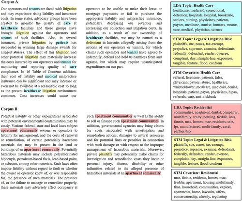
The text corpora (corpus A and B) in Figure 1 illustrate examples of our later-used data set. The identified words defining the topics by LDA correspond to the already known sectors – corpus A is provided by a firm in the healthcare sector and corpus B by a firm in the residential sector. At the same time, both corpora address the topic ‘Legal & Litigation Risk’ which is not identified by LDA but by STM as the common topic. Thus, STM allows extracting common factors across documents by excluding the already known metadata (e.g. healthcare and residential) and their corresponding words. Consequently, the industry-specific vocabulary distracts the LDA and CTM from extracting common risk factors.

This research delves into the question of whether risk topics, extracted from unstructured text data using advanced machine learning methods, yield more effective results in explaining return volatility compared to older methods that focus on text length and readability, or overlook the correlation between topics and words in documents. Our aim is to contribute to the growing utilization of text data in accounting and financial research. Additionally, we seek to shed light on the unresolved question of whether the capital market perceives it positively (i.e. risk-minimizing) when firms provide more comprehensive disclosures about risks in their documents.

We find that LDA and CTM are distracted from extracting common risk factors and can therefore hardly be linked to the pricing behavior of investors. Contrary, the STM-extracted risk factors are statistically significantly associated with volatility and consequently, with the risk perception of investors. Simple methods of measuring risk by counting words are of minor importance but a hybrid model – combining machine learning with a word-counting factor – explains best the return volatility within our dataset. Our results mostly support that executives use disclosures to resolve firms’ known risk factors or give more facts about known risk factors and thus, reduce risk perceptions on the market. In a supplementary analysis, we discover supporting evidence for extending our findings also to sectors with heterogeneous business models and lower investor perception.

Our findings carry implications for the accounting and finance research community, as well as for industry practices. By leveraging advanced machine learning-based methods that consider the covariate and covariance aspects of words, we can effectively identify risk-relevant factors from textual data. This capability enables us to incorporate information into our risk analyses that would otherwise be hard to include, given the limitations of human capacity to process thousands of documents. The observed predominantly risk-reducing effect associated with a higher likelihood of occurrence of risk topics may serve as motivation for firm executives to enhance the discussion of risk factors in their disclosures. This could potentially clarify the impact of risks on the firm’s future development.

Our study contributes to the literature in various ways. To the best of our knowledge, this is the first study applying STM to the accounting and finance domain while also benchmarking it with LDA and CTM. We show, that the so-far predominantly used LDA is biased by the used idiosyncratic language within an industry reflecting rather the already known operative line of business or business models than significant topics of a document. This is also true for CTM, the advanced LDA algorithm, which is the most suitable benchmark for STM although it is not used in the economic literature so far. In addition, our analysis provides insights into whether and how information is incorporated into the pricing process. By introducing STM, we apply the algorithm to the important but rather neglected industry sector of REITs (Real Estate Investment Trusts). This industry is an appealing testing ground for multiple reasons. First, while the sector is described by relatively homogenous business models and firm characteristics, its firms invest in different property types (e.g. healthcare, residential). This sample allows us to show that even in a sample favorable to LDA, it is more likely to find already known topics (i.e. property types) rather than uncovering common risk factors across the entire sector. In contrast, STM has the capability to directly discern these shared risk factors. Second, REIT’s managers must turn to the capital markets repeatedly to raise funding for new projects since they have very limited cash reserves due to regulation requirements. This regulation incentivizes REITs to be transparent, disclose their fillings with a relatively high quality, act for the long-term, and sustain investor trust. Third, REITs are distinguished by substantial investments in fixed assets, resulting in relatively stable cash flows. This stability appeals to institutional investors, equipped to navigate through lengthy and intricate disclosures more effectively. Therefore, it is reasonable to anticipate observable stock market reactions based on the disclosed information for this sector.

The remainder of the paper is organized as follows. Section 2 discusses related literature on mandatory risk disclosures and develops hypotheses. Section 3 explains the textual analysis procedures (i.e. LDA, CTM, and STM) and the empirical model, while Section 4 introduces the data used and describes the variables. The empirical results are reported in Sections 5 and 6 concludes.

2. Previous literature and hypotheses development

2.1. Textual analysis in accounting and finance

Fueled by the rise of computational power and the tremendously increasing online availability of text, a growing body of literature in accounting and finance has focused on computer-based techniques to find and quantify information revealed in qualitative disclosures (e.g. media news, public corporate disclosures, analyst reports, and internet postings). Within the finance research, probably Tetlock (2007) provides the pioneering study by employing automated content analysis to extract sentiment from the Wall Street Journal’s column ‘Abreast of the Market’ by counting specific words. He demonstrates, that media pessimism induces downward pressure on market prices and leads to temporarily high market trading volume. Thereafter, multiple studies analyze how sentiment predicts the reactions of financial markets. For example, Garcia (2013) processes finance news from The New York Times and provides evidence that positive words also help to predict stock returns. Tetlock, Saar-Tsechansky, and Macskassy (2008) analyze firm-specific news from the Dow Jones News Service and The Wall Street Journal and prove that negative words convey negative information about firm earnings beyond stock analysts’ forecasts and historical accounting data. Antweiler and Frank (2004), Das and Chen (2007), and Chen et al. (2014) investigate the textual sentiment of internet messages. Hereby, Antweiler and Frank (2004) find evidence that the amount of message posting predicts market volatility and trading volume. Chen et al. (2014) figure out that the fraction of negative words contained in articles published on Seeking Alpha negatively correlates with contemporaneous and subsequent stock returns. Das and Chen (2007) make assumptions about the relationship between textual sentiment and investor sentiment when interpreting textual sentiment or tone of internet messages as small investor sentiment. They link market activity to small investor sentiment and message board activity. Regarding the studies addressing corporate disclosures, textual sentiment has been found to be positively related to abnormal stock returns (e.g. Chen et al. 2014; Feldman et al. 2010; Jegadeesh and Wu 2013), subsequent stock return volatility (e.g. Loughran and McDonald 2011; 2015), and future earnings and liquidity (e.g. Li 2010).

Further research investigates the readability of corporate disclosures and provides evidence that lower annual report readability is associated with increased stock return volatility (Loughran and McDonald 2014), lower earnings persistence as well as higher earnings surprise (Li 2008; Loughran and McDonald 2014), larger analyst dispersion (Lehavy, Li, and Merkley 2011; Loughran and McDonald 2014), and lower trading due to a reduction in small investor trading activity (Miller 2010). Only recently, Cohen, Malloy, and Nguyen (2020) use sentiment and multiple similarity measures to show that changes to the language and construction of corporate disclosures impact stock prices with a time lag. The authors conclude that investors need time to process complex and lengthy disclosures.

Other recent papers try to develop new machine-learning-based methods for textual comprehension and topic extraction in financial economics. Among them, Cong, Liang, and Zhang (2019) generate textual factors using neural-network language processing and generative statistical modeling which can be used for macroeconomic forecasting and factor asset pricing. Kelly, Manela, and Moreira (2021) develop a high-dimensional selection model that focuses more on a phrase than the frequency of repetition. They apply it not only to U.S. congressional speeches but also to estimate macroeconomic indicators using newspaper text. Li et al. (2021) create a culture dictionary based on the word embedding model and earnings call transcripts and show that an innovative culture is wider than the usual way to measure innovation. Das et al. (2022) present an automated approach to generate wordlists that have a comparable performance to traditional lists on machine learning classification tasks.

This study contributes to the emerging literature on textual analysis by adopting a new perceptive based on an often applied method. Instead of focusing on the tone conveyed through the narrative, the complexity of the language, or document similarity, we extract topics out of corporate risk disclosures using machine learning approaches.

2.2. Textual analysis of risk disclosures

The literature has applied various methods to assess a firms’ risk disclosure, which we classify in two categories. Within the first and more straightforward category, the entire risk disclosure is observed as a unit and its ‘size’ is considered as a proxy for risk. Within the second and more sophisticated category, the individual risk itself comes to the forefront. The former category comprises studies that count risk keywords (e.g. Kravet and Muslu 2013; Li 2006) or rely on the total length of the risk section (e.g. Campbell et al. 2014; Nelson and Pritchard 2016) to measure firms’ risk disclosures. Hereby, increased levels of forward-looking disclosures (e.g. risk disclosures) are linked to an increased trading volume (Kravet and Muslu 2013), and lower future earnings and stock returns (Li 2006). The result for stock return volatility is not so clear; the majority find a decreasing effect (e.g. Beyer et al. 2010; Muslu et al. 2015), whereas others an increasing effect (e.g. Campbell et al. 2014; Kravet and Muslu 2013). Common to the studies using straightforward approaches is that they can process a large number of textual documents which is beyond human capacity, but they obviously lose a lot of information written in the text.

Only recently and within the latter category, researchers have started to focus more on the written content by making use of machine learning approaches to identify and quantify the individual risks. In this context, the unsupervised machine learning approach Latent Dirichlet Allocation (LDA) is most popular for finding the individual risks discussed in firms’ filings. The outcomes are manifold: Israelsen (2014), for example, examines the association between the risks disclosed in Item 1A and stock return volatility, as well as betas of the Fama-French Four-Factor model. Employing a variation of the LDA, Bao and Datta (2014) analyze whether and how risk disclosures affect investor risk perceptions. Their findings indicate that some risk factors increase or decrease investor risk perceptions, and thus lead to higher or lower post-filing return volatility, whereas the majority have no effect at all. Gaulin (2019) uses disclosed risk factors to analyze disclosure habits and suggests that managers time the identification of new risks, as well as the removal of previously identified ones, to match their expectations of adverse outcomes in the future. Recently, Lopez-Lira (2023) demonstrates the importance of risk disclosures by providing a factor model that uses only identified firm risk factors to explain stock returns and performs as least as well as traditional models, without including any information from past prices.

The key benefit of machine learning approaches is that they do not require predefined rules (i.e. a priori determined keywords) to identify risk factors. Instead, risk factors or general speaking topics derive naturally from fitting the statistical model to the textual corpus, based on word co-occurrences in the documents.

2.3. Hypotheses

Common to all approaches, whether straightforward or sophisticated, is that they attempt to quantify qualitative information in disclosures without the need for a human being to read them. However, quantifying risk disclosures is quite challenging given that firms neither reveal the likelihood that a disclosed risk will ultimately affect the company, nor the quantified impact a risk might have on the firm’s current and future financial statements. Thus, forward-looking risk disclosures might inform the reader, for the most part about a vague range, but certainly not the level of future performance (Kravet and Muslu 2013). Nevertheless, assuming that firm executives truthfully report their views under SEC scrutiny and penalty of litigation, it can be argued that detailed firm-specific information is provided in 10-K filings. In fact, previous research (e.g. Bao and Datta 2014; Kravet and Muslu 2013) finds a stock market reaction of risk disclosures confirming its informativeness.

Recognizing that management’s discretion entails considerable leeway in deciding which information about a risk factor is disclosed and how much of the filing is allocated to a particular risk-factor topic, we assume that these probabilities of topics provide valuable information on how companies assess the extent of the risks. Accordingly, the topic probabilities in the filings derived from unsupervised machine learning algorithm, mostly by the Structural Topic Model (STM), could serve as a proxy for risk beyond the level of previous straight-forwarded proxies (e.g. word count, text length), allowing investors to quantify the information provided in narrative form.

Hypothesis 1: The probabilities of risk topics in textual reports – derived from the STM model – present significant explaining factors in empirical models analyzing investor risk perception.

The nature of risk disclosures is that it explains but does not necessarily resolve uncertainties. Thus, theoretic models (e.g. Cready 2007; Kim and Verrecchia 1994) see the possibility that risk disclosures increase or decrease investors’ risk perceptions. Kravet and Muslu (2013) define three opposing arguments. The first argument suggests that investor risk perceptions remain unaffected since risk disclosures are vague and use boilerplates because managers are likely to report all possible risks and uncertainties without considering their impact on businesses just to be on the safe side (null argument). The second argument states that risk disclosures reveal unknown risk factors or risk-increasing facts about known risk factors causing diverging investor opinions and increasing risk perceptions (divergence argument). The third argument assumes that executives use disclosures to resolve firms’ known risk factors or give more facts about known risk factors and thus, reduce risk perceptions (convergence argument). This ambiguity is supported by the mixed results in empirical research (see the previous subsection), whereas the majority find resolved uncertainties (i.e. lower volatility) in response to corporates’ disclosures. Since we are able to extract risk topics at a higher level of granularity than previous straight-forwarded risk proxies, we assume that we find all three risk perceptions (null, convergence, and divergence argument). Knowing that the annual frequency of 10-Ks is from the legal and practical perspective inappropriate to discuss new risks, we assume that the majority of disclosures resolve known risk factors and contingencies and formulate our next hypothesis as follows.

Hypothesis 2: The majority of the risk factors present a risk-reducing effect, supporting the convergence argument.

3. Model design

3.1. Textual analysis with machine learning: LDA and CTM

Topics derive naturally from fitting the statistical model to the textual corpus based on word co-occurrences in the documents. Thus, this procedure eliminates subjectivity that would otherwise be introduced by predefined wordlists, and yet provides more informative results than straight-forwarded approaches, which can still be interpreted economically. The Latent Dirichlet Allocation (LDA) is the most frequently used topic modeling approach in the scientific literature; it is borrowed from genetic science (Pritchard, Stephens, and Donnelly 2000) and transferred to machine learning by Blei, Ng, and Jordan (2003). It is a mixture model, generating the probabilities of co-occurring topics (subpopulation) within the distribution over all words (population). Put simply, the mixture model aims to break documents down into topics, whereby the words within each topic co-occur most frequently. Thus, applying the LDA to a textual corpus results in two data structures in the output. The former presents the probability of appearance of each topic in each document (${\theta }_d$), with documents being indexed by $d$. The latter lists a set of words and their probabilistic relation with each of the extracted topics (${\beta }_k$), with topics being indexed by $k$.

LDA comes with the limitation that the used Dirichlet distribution assumes almost uncorrelated topics. However, they are likely correlated in reality since particular topics occur at the same time. For an illustration, see Figure 1 in our Introduction. These covariances are addressed by Blei and Lafferty (2007) in their Correlated Topic Model (CTM) method. Also, the CTM is a mixture model but replaces the Dirichlet distribution with a logistic normal distribution in order to include the covariance structure among topics. Surprisingly, it is not very often applied even if Blei and Lafferty (2007) show the theoretical and practical importance of a covariance structure by using 16,351 Science articles. They find that CTM is always superior to LDA for altering the number of topics from 5 to 120.¹

3.2. Textual analysis with machine learning: STM

The Structural Topic Model (STM) by Roberts, Stewart, and Tingley (2019) goes even one step further and incorporates metadata of pre-specified covariates (industry-specific vocabulary), not only covariances; see Figure 1 and discussion in the Introduction for healthcare vs. residential. Again, it remains a mixture model based on a logistic normal distribution, so that it corresponds to CTM if covariates are ignored. The covariates cover for topical prevalence, topical content, or both. The former affects how much a topic is discussed (${\theta }_d$), whereas the latter affects which words are used to discuss a particular topic parameter (${\beta }_k$) (Roberts et al. 2014). In order to allow the algorithm to find topics beyond the already known identifiers, we include property types as metadata covariates. Contrary to the LDA, where the topic proportion ${\theta }_d$ is drawn from a Dirichlet distribution, the STM employs a logistic-normal generalized linear model which is based on document covariates ($X_d$). Thus, the frequency with which a topic is discussed that is common across all documents in the LDA is now affected by the observed metadata, as indicated by the following equation: (1) ${\overrightarrow{\theta }}_d|X_d\gamma ,\mathrm{\Sigma }\sim \mathrm{LogisticNormal}(\mu =X_d\gamma ,\mathrm{\Sigma }),$(1) where $X_d$ is a 1-by-$p$ vector, $\gamma$ is a $p$-by-$(K-1)$ matrix of coefficients and $\mathrm{\Sigma }$ is $(K-1)$-by-$(K-1)$ covariance matrix.

Whereas LDA assumes that word proportions within each topic ($k$) are represented by the model parameter ${\beta }_k$, which is identical for all documents ($d$), STM allows that the words describing a topic vary. Specifically, given a document-level content covariate $y_d$, the STM forms document-specific distributions of words representing each topic ($k$) based on the baseline word distribution ($m$), the topic-specific deviation $K_k$, the covariate group deviation $K_{y_d}$, and the interaction between the two $K_{y_d,k}$. 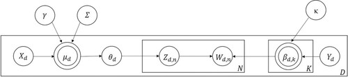The following equation provided by Kuhn (2018), and based on Roberts, Stewart, and Tingley (2019), summarizes this relationship as follows: (2) ${\beta }_{d,k}\propto \exp (m+K_k+K_{y_d}+K_{y_d,k})$(2) Figure 2 presents the STM in the common plate notation for topic modeling. Hereby, one ‘plate’ exists for each document $(D)$ and its associated topic distribution $({\theta }_d)$ in the textual corpus. The inner plate, comprising topics $(Z_{d,n})$ and words $(W_{d,n}),$ is replicated for each of the $N$ words in the document. Analogously, the plate including the model parameter ${\beta }_{d,k}$ is replicated for each of the $K$ topics in a textual corpus (Blei 2012; Kuhn 2018)

Figure 2. Structural topic modeling, in plate notation (following Roberts, Stewart, and Tingley 2019).

After pre-processing, we estimate the STM, based on a variational Expectation-Maximization algorithm. The maximum number of iterations is set to 100, so that convergence is always reached before this threshold.

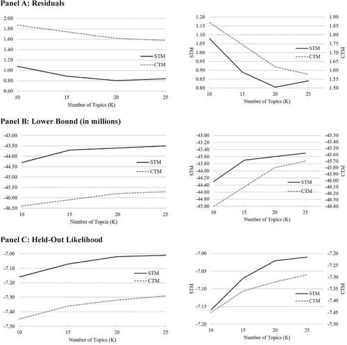
We run various tests checking whether the higher flexibility of STM corresponds to a better fitting among the approaches. The better the topic identification works the higher the probability that the topics may help to explain the investors’ risk perception. In a pre-test, we run a technical comparison for CTM and STM similar to Blei and Lafferty’s (2007) comparison for LDA and CTM. We fit a smaller collection of documents of our later-used dataset to a varying number of topics (between 10 and 25) and calculate the residuals, lower bounds, and log likelihoods of the held-out data. The better a model fits the lower are the residuals and the higher are the lower bounds as well as the probability of the held-out data. All three measures indicate a better fit for STM for the full range of topic numbers (see Figure 3, Panel A-C). Additionally, topic modeling requires an a priori determination of the number of topics to be generated. All comparison measures indicate directly or converge to a topic number of 20 as the best number. Consequently, we extract 20 individual risk factors from the risk disclosures.

Figure 3. Comparison of CTM and STM.

This figure shows the standard criteria for comparing different topic models, namely residuals regarding the text corpora (Panel A), lower bound (Panel B), and held-out likelihood with a standard of 20 percent (Panel C). On the left hand side and identical scale, the STM outperforms the CTM on our data set. The right side shows two different scales for each model to clarify the turning points of optimization process for a different number of topics (K) within each model.

Based on the superiority of CTM over LDA (see Blei and Lafferty 2007) and STM over CTM as well as LDA (see Roberts et al. 2014 and our pre-test), we assume that STM is most suitable to extract topics explaining the investors’ risk perception. In our later analysis (Subsection 5.5), we compare the explanatory power of all three approaches to explain the investors’ risk perception.

3.3. Topic identifications: pre-steps

Several preprocessing steps are necessary before running the topic models. First, we parse the downloaded 10-K filings to extract the risk report part from the entire document.² In addition, we clean the data by removing spaces, numbers, and punctuation. Second, relying on the ‘stop word’ list provided by Grün and Hornik (2011) and Roberts, Stewart, and Tingley (2019), words like ‘and’, ‘or’, and ‘the’ are removed from the corpus, since they lack semantic information, and thus do not help to identify the topics. Third, we eliminate words appearing in fewer than 20 disclosures to avoid their influence. On the one hand, this threshold (20 occurrences) rules out words occurring solely in 10-K filings of one particular firm (e.g. the firm names), since we have 14 years of observations. On the other hand, low-frequency words cannot be clearly assigned to an individual topic, and thus introduce noise into the process. Excluding them ensures the robustness of the algorithm, and in addition, increases computational speed (Papilloud and Hinneburg 2018). Unlike Roberts, Stewart, and Tingley (2019), we do not stem the words and instead use explicit word inflections for reasons of interpretability. This abandonment is supported by Schofield and Mimno (2016), who find that stemming does not improve topic stability, and possibly even degrades it.

3.4. Topic identifications: risk factors labeling

Although topic-modeling approaches classify textual data without further instruction by the user, the topics created by the algorithms (LDA, CTM, and STM) do require an interpretation. More specifically, a human being has to assign labels with an assessment of the most plausible content to the algorithm-based topics, which are only equipped with a number and a set of words most frequently associated with each topic.

In order to label the risk-factor topics appropriately, we read a random sample of disclosures comprising 2% of the overall sample. Two of us then independently reviewed the word lists comprising the 20 highest associated terms for each risk-factor topic. As recommended by Roberts, Stewart, and Tingley (2019), we also inspected documents that were considered to be highly associated with a specific topic, and thus, are expected to represent the topic most clearly. We discuss the associated words selected labels in Subsection 5.4. Table A.1 in Appendix A presents the full list of the 20 highest associated words for each risk factor topic for STM and the corresponding name; Table B.1 in Appendix B does it for LDA.

3.5. Risk model specification

Drawing on prior research investigating the associations between risk disclosures and stock return volatility (e.g. Bao and Datta 2014; Kravet and Muslu 2013), we construct a model that incorporates various potential risk factors. These factors include textual data obtained through machine learning methods (e.g. Bao and Datta 2014; Israelsen 2014; Muslu et al. 2015), textual data derived from simple counting methods (e.g. Campbell et al. 2014; Lehavy, Li, and Merkley 2011; Li 2008), changes in performance, ownership, trading volume, firm-specific and market-wide risk measures (e.g. Bamber and Cheon 1995; Kim and Verrecchia 1991; Kravet and Muslu 2013), and REIT-specific risk factors taking into account that REIT’s returns have become sensitive to factors influencing small-cap stocks (e.g. Bond and Xue 2017; Ooi, Webb, and Zhou 2007). With the exception of the first category, all other variables are grouped within the control variables category. A detailed description of the independent variables is provided in Subsection 4.3.

To assess whether the probabilities of appearance of the extracted risk factors helps to explain the perceived risk on the stock market, we regress whose frequencies ($\mathrm{Freq}\mathrm{\_Topics}$) on the firms’ stock return volatility ($\mathrm{Vola}$) by using the following two-way fixed-effects regression model: (3) $\mathrm{Vol}{a}_{\mathrm{it}}={\beta }_0+{\beta }_1\mathrm{Freq}\mathrm{\_Topic}{s}_{\mathrm{it}}+{\beta }_2\mathrm{Control}{s}_{\mathrm{it}}+a_i+{\lambda }_t+u_{\mathrm{it}},$(3) where $i$ denotes the firm, and $t$ the year. In addition to the vector of the distribution of the individual risk topics ($\mathrm{Freq}\mathrm{\_Topics}$), the regression equation includes a vector of control variables ($\mathrm{Controls}$). The parameters $a_i$ and ${\lambda }_t$ incorporate the unobserved firm and time effects and $u_{\mathrm{it}}$ is the error term. The two-way fixed effects model incorporates the specific differences between individuals in a micro panel dataset covering roughly 14 years (Wooldridge 2010). To produce consistent, efficient, and unbiased estimates, we examine whether any of the models’ assumptions are violated. Employing Variance Inflation Factors (VIF) to check for multicollinearity, we find values greater than 5 for Topic #7, Topic #11, Topic #14, and Topic #18. Thus, these topics are explained by all other topics by at least 80% each, so we exclude these topics from our later analysis. In doing so, we apply a stricter threshold often applied (greater than 10 or 90% is explained by the other topics), since we prefer to have a parsimonious model with fewer variables, which make it less susceptible to spurious relationships and harder to verify that our topics are significant. The VIFs of the remaining variables are within the range of 1.1 and 4.4.

4. Data

4.1. Data source and sample

To test our hypotheses, we combine multiple datasets: (1) investors’ risk perception proxied by stock return volatility from CRSP, (2) the text corpus given by the Risk Factor report (Item 1A) of the annual 10-Ks obtained from the Electronic Data Gathering and Retrieval (EDGAR) database, and (3) firms’ financial and accounting fundamentals obtained from Compustat or Thomson Reuters.

Our sample begins with the earliest date when ‘Item 1A. Risk Factors’ was available (1 December 2005)³ and extends through the fiscal year-end 2019. To mitigate potential confounding factors related to the pervasive risk associated with the COVID-19 pandemic, we concluded our sample in 2019. This deliberate decision ensures the avoidance of any overlap with the pandemic's impact on our analysis. In contrast to other studies focusing on the entire firm-year sample available from the EDGAR database, we limit our examination to a single industry, namely the REIT industry, for multiple reasons. First, while the sector is characterized by relatively homogenous business models and firm characteristics, different investment foci in property types (e.g. healthcare, residential) are salient and distract the LDA from extracting common risk factors (see Figure 1). Second, REITs’ 10-Ks guarantee a relatively high disclosure quality, given their high dividend payout requirement of at least 90% of their taxable earnings. Consequently, they have a very limited cash reserve and must turn to the capital markets repeatedly to raise funding for new projects. This regulation incentivizes that REITs are transparent, act for the long-term, and sustain investor trust (Danielsen et al. 2009; Doran, Peterson, and Price 2012; Price, Seiler, and Shen 2017). Third, the real estate industry is characterized by a well-known business model – high investments in fixed assets generate relatively constant cash flow for their investors. This property is attractive for institutional investors since the early 1990s as shown by others (e.g. Lee, Lee, and Chiang 2008; Ling and Ryngaert 1997). This type of investor can process lengthy and complex disclosures easier, so it is reasonable to assume that we can observe stock market reactions based on the disclosed information. Furthermore, investors must intensively monitor this type of industry for adverse information and outcome (risk) since their capital is tied in fixed assets, which do not have high future expectancies regarding new technologies or where losses can be compensated by new exceptional growth opportunities. In addition, institutional investors are rarely driven by noise trading or herding behavior, which irrationally influence the stock prices. However, institutional investors apply often passive investment styles with a buy-and-hold strategy and a long-term horizon (see e.g. Chung, Fung, and Hung 2012; Devos et al. 2013). Consequently, positive news keeps the ownership of institutional investors constant whereas negative news may not lead to a direct divestment if they are not severe.

Our sample consists of all Equity REITs present in the FTSE NAREIT All REITs Index at any point of time during the sample period. Mortgage REITs are excluded from the analysis because they differ in characteristics (e.g. underlying asset, risk structure), exposed risk factors, and are recognized as more difficult to value for external investors (Buttimer, Hyland, and Sanders 2005). Out of the 246 distinct firms, 25 consistently remain in the index throughout the entire sample period, while 221 firms either enter, exit, or both enter and exit the sample. After including control variables, our subsequent regression analyses are based on 199 distinct firms. Figure 4 displays the sample composition of the 10-Ks over years; our observations mostly follows the number of REITs included in the FTSE NAREIT All REITs Index over the same time period. For some years, the observations exceed the number of index constituents, since we include a firm in our sample if it was a constituent at any point during the period. We thus address survivorship bias and index effects such as greater investor attention to firms listed in an index. Firm-year observations that lack necessary control variables or stock prices are excluded, resulting in an overall sample of roughly 1,230 observations consisting of 199 unique firms. The limiting variables are the control variables obtained from CRSP and Compustat and not the risk factors extracted from the 10-K filings (see Table 1 for more details about N).

Figure 4. Sample distribution over years.

This figure shows the number of observations included in the sample and the number of Equity REITs present in the FTSE NAREIT All REITs Index over years.

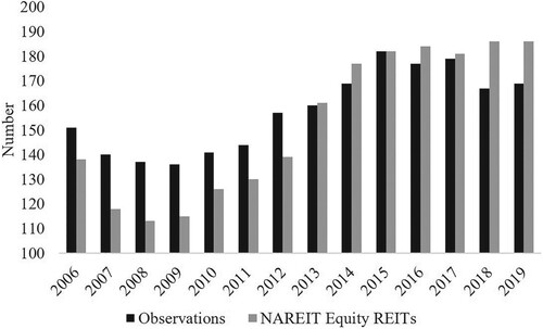
Table 1. Descriptive statistics.

	N	Mean	StDev	Min	Q1	Median	Q3	Max
Item 1A
Freq_Topic 1	2,207	5.121	20.447	0.000	0.003	0.007	0.017	99.940
Freq_Topic 2	2,207	5.043	20.626	0.000	0.003	0.007	0.020	99.934
Freq_Topic 3	2,207	2.441	13.409	0.000	0.008	0.018	0.055	99.773
Freq_Topic 4	2,207	3.968	17.793	0.000	0.004	0.012	0.036	99.901
Freq_Topic 5	2,207	3.475	16.227	0.000	0.005	0.014	0.044	99.835
Freq_Topic 6	2,207	4.828	19.686	0.000	0.003	0.009	0.020	99.934
Freq_Topic 7	2,207	3.715	17.584	0.000	0.004	0.010	0.025	99.894
Freq_Topic 8	2,207	4.317	18.118	0.000	0.007	0.014	0.043	99.877
Freq_Topic 9	2,207	4.883	20.521	0.000	0.004	0.008	0.020	99.978
Freq_Topic 10	2,207	4.813	16.571	0.000	0.011	0.024	0.116	99.870
Freq_Topic 11	2,207	3.330	15.479	0.000	0.004	0.009	0.025	99.959
Freq_Topic 12	2,207	6.648	23.855	0.000	0.002	0.008	0.024	99.939
Freq_Topic 13	2,207	6.406	22.932	0.000	0.004	0.009	0.028	99.932
Freq_Topic 14	2,207	2.221	13.626	0.000	0.001	0.004	0.012	99.973
Freq_Topic 15	2,207	5.477	21.310	0.000	0.004	0.009	0.022	99.952
Freq_Topic 16	2,207	7.566	25.358	0.000	0.003	0.008	0.019	99.939
Freq_Topic 17	2,207	6.527	23.341	0.000	0.004	0.009	0.023	99.939
Freq_Topic 18	2,207	7.043	23.956	0.000	0.004	0.012	0.036	99.983
Freq_Topic 19	2,207	6.913	23.799	0.000	0.003	0.009	0.025	99.975
Freq_Topic 20	2,207	5.265	21.145	0.000	0.004	0.008	0.020	99.931
Control Variables
FFO/Share	1,861	1.986	4{,}114	−18.258	0.593	1.385	2.579	127.368
Size	2,020	7.759	1.314	−1.931	7.106	7.907	8.558	10.556
Leverage	2,020	0.566	0.181	0.000	0.473	0.560	0.660	1.638
$\mathrm{\Delta }$REV	1,876	47.207	204.435	−4{,}403.782	1.039	21.619	68.020	3{,}701.640
Sales_Growth	1,862	0.034	0.436	−0.800	0.001	0.011	0.027	16.478
Beta	1,892	0.974	0.495	−0.692	0.622	0.927	1.259	4.661
BTM	1,956	−0.116	3.018	−64.892	−0.049	0.0002	0.001	75.038
IO	1,749	0.760	0.283	0.000	0.637	0.838	0.954	2.383
Vola^S&P (−5, 0 days)	1,543	0.019	0.012	0.002	0.010	0.017	0.025	0.082
Vola^S&P (−40, 0 days)	1,537	0.056	0.030	0.025	0.038	0.047	0.056	0.175
Vola^S&P (−60, 0 days)	1,535	0.068	0.031	0.030	0.052	0.056	0.078	0.193
$\mathrm{\Delta }$Volume (0, 5 days)	1,543	0.119	0.893	−4.306	−0.049	0.025	0.183	20.333
$\mathrm{\Delta }$Volume (0, 40 days)	1,529	0.052	0.545	−2.601	−0.085	0.001	0.095	7.790
$\mathrm{\Delta }$Volume (0, 60 days)	1,519	0.050	0.520	−2.860	−0.082	0.003	0.100	7.646
Text_Length	2,207	68,231	50,034	36	38,302	57,270	87,198	516,463
FOG	2,207	22.460	1.707	5.000	21.665	22.496	23.307	29.698
Dependent Variables
Vola (0, 5 days)	1,543	0.041	0.047	0.001	0.020	0.032	0.047	1.125
Vola (0, 40 days)	1,537	0.116	0.123	0.030	0.071	0.085	0.110	2.119
Vola (0, 60 days)	1,535	0.142	0.132	0.033	0.088	0.107	0.141	2.130

This table shows the descriptive statistics for the frequencies (in %) for the risk factor topics (Freq_Topic) of Item 1A, further control variables, and dependent variables (Vola). The definition of all variables is presented in Table A.3 in Appendix A. N is the number of observations, StdDev stands for standard deviation, Q1 is the first and Q3 the third quartile of the distribution, and Min is the minimum and Max the maximum of each variable. N is set to the maximal available number of observations for each variable.

4.2. Investors’ risk perception

The dependent variable of interest is the perceived risk on the stock market measured by the return volatility after the filing date using the daily closing prices from CRSP. It is unclear how long it takes until investors read 10-Ks, and new information is incorporated into price changes. Thus, we apply multiple testing periods for firms’ stock return volatility after the 10-K filing is published – a 5, 40, and 60 trading-day period. The 5 trading-day period gives investors enough time to read, interpret and react to disclosures while being short enough to minimize the influence of other disruptive events that may also affect volatility. The 60 trading-day period accounts for investors comparing risk factors disclosed in 10-Ks to changes disclosed in quarterly reports (10-Qs).⁴ We calculate volatility as the standard deviation of daily log returns extrapolated to the 5, 40, and 60 trading-day periods after the 10-K filing day. (4) $\mathrm{Vol}{a}_T=\sqrt{T}\ast \sqrt{\frac{{\sum }_{t=1}^T{(\ln (1+r_t)-{\mu }_T)}^2}{T-1}},$(4) where $\mathrm{Tϵ}\{5,40,60\}$.

In contrast to the common approach using a 252 trading-day volatility, our procedure concentrates on the volatility induced by the information released in the 10-K. A 252 trading-day window may be too diluted since it includes price-sensitive information over the entire prior trading year. Thus, past information that is already known and has been incorporated into prices, would be extrapolated to our testing period. Additionally, the standard deviation over a 252 trading-day window would cause autocorrelation problems after adding a control variable for the lag volatility for the days before the 10-K filing date, since the majority of the time window overlap. We illustrate this in Figure 5, Panel A.

Figure 5. Volatility around publication date.

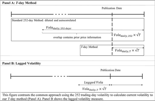
By contrast, our method surveys volatility, starting from the filing publication date until the end of the processing period. To account for the problem of autocorrelation due to volatility clustering around specific dates and other influencing filing events, we include a lagged volatility measure in the model as a control variable. This variable gauges the standard deviation $T$ days before the publication date, see Figure 5, Panel B. We also attempted to utilize alternative risk measures, such as implied volatility based on options and credit default spreads. However, we faced difficulties in acquiring an ample number of observations for our subsequent analyses, and consequently, we have retained volatility as our risk measure.

4.3. Independent variables

Our primary influencing variables of interest are the frequencies of the machine learning-extracted risk factors discussed in corporate disclosures ($\mathrm{Freq}\mathrm{\_Topic}$). We start with the STM and verify our results using CTM and LDA; their calculations are described in Section 3. To control for information beyond the risk factors, a set of control variables is included. Besides firm characteristics, performance, and risk measures, we additionally consider textual 10-K characteristics that previous research has revealed as determinants of return volatility. We describe all control variables below, and provide more specific definitions, including Compustat data items, in Table A.3 in Appendix A. We cluster the controls into two subsets: (1) accounting-based/market-based and (2) textual.

For the first of the two, we include the REIT-specific performance measure Funds From Operations per share ($\mathrm{FFO}/\mathrm{Share}$), to incorporate the real-estate-specific income characteristics. We calculate $\mathrm{FFO}$ by following NAREIT’s guideline: the sum of net income, amortization & depreciation, and the difference of the net of gains and losses originated by the sale of assets from the net income. Since $\mathrm{FFO}/\mathrm{Share}$ is a performance measure, we expect a negative coefficient sign. The variable $\mathrm{Size}$, measured as the natural logarithm of the firm’s total assets, controls for Fama and French’s (1993) finding that small firms are more volatile than large firms; we expect its coefficient to be negative. $\mathrm{Leverage}$ is a common proxy for firm risk, so we expect the variable to be positively related to volatility. The motivation for the next two factors is purely at the operating level – the annual change in revenue ($\mathrm{\Delta }\mathrm{REV}$) as well as sales growth ($\mathrm{Sales}\mathrm{\_Growth}$). $\mathrm{\Delta }\mathrm{REV}$is defined as current sales or rental income less prior year sales.$\mathrm{Sales}\mathrm{\_Growth}$is calculated as $\mathrm{REV}$ scaled by total assets in the previous year. We expect a positive influence from both variables. Among the market-based controls, $\mathrm{Beta}$ proxies the firm risk similar to $\mathrm{Leverage}$, so that we expect a positive nexus to volatility. Book-to-Market $(\mathrm{BTM})$ is calculated as the book value of equity, scaled by the market capitalization of equity. Our expectations of $\mathrm{BTM}$ are ambiguous. On the one hand, the coefficient could be positive if market participants have little confidence in the future prospects of a firm. On the other hand, the coefficient on $\mathrm{BTM}$ will be negative if growth opportunities are positively related to firm risk (Campbell et al. 2014; Fama and French 1993). The standard control variables, BTM and Size (natural logarithm of total assets), are employed independently of the Fama-French methodology. This is crucial, as early analyses of REITs revealed that their return characteristics, predominantly influenced by stable cash flows, bear a closer resemblance to bonds than to stocks (Karolyi and Sanders 1998). Consequently, it comes as no surprise that Fama and French (1993) excluded REITs, along with other financial firms, from their dataset. However, the REIT landscape had undergone significant structural changes in the early 1990s, reshaping them into instruments that bore a closer resemblance to stocks (Glascock, Lu, and So 2000). This transformation prompted a shift in research, revealing that REIT returns became increasingly responsive to the same factors influencing small-cap stocks and specific drivers within the real estate sector (Clayton and MacKinnon 2003). As a result, contemporary research has adopted Size and Book-to-Market as risk factors to elucidate the dynamics of REIT returns (e.g. Bond and Xue 2017; Ooi, Webb, and Zhou 2007).

Additionally, we include the stock return volatility ($\mathrm{Lag}\mathrm{\_Vola}$) for the corresponding $T$ trading-days before the 10-K filing date, to control for positive volatility correlation in the short-run and information released in other outlets as the 10-K. We expect a positive relationship between the pre – and post-filing-date volatility. We also add the stock return volatility of the S&P 500 (Vola^S&P) for $T$ trading-days before the 10-K filing date, as a benchmark for changes in the general market volatility and expect a positive coefficient. The change of a firms’ average daily trading volume from the symmetric period of $T$ trading-days before to after the 10-K is filed ($\mathrm{\Delta }$Volume), serves as a factor of the economic interactions in the financial market. In addition to stock price changes, trading volume conveys important information about the underlying economic forces. We expect that higher changes in the trading volume go in line with higher volatilities. Furthermore, the percentage of institutional ownership ($\mathrm{IO}$), defined as the sum of shares held by institutional investors, divided by the shares outstanding, is incorporated as obtained from Thomson Reuters. Institutional investors have higher capacities to process 10-Ks, and thus could react in a timely manner to the disclosed information, causing a positive coefficient on $\mathrm{IO}$. Conversely, the coefficient could be negative if the long-term orientation of sophisticated investors is predominant and they behave inertially.

For the second subset of controls, we include straight-forwarded textual content measures of previous research. In line with Campbell et al. (2014) who show that the number of words is positively related to stock return volatility, we incorporate the natural logarithm of the total text length of the risk sections ($\mathrm{Text}\mathrm{\_Length}$). Additionally, we follow Li (2008) and Lehavy, Li, and Merkley (2011) and incorporate the readability measured by the Gunning fog index ($\mathrm{FOG}$) to account for higher information-processing costs of complex language.

4.4. Descriptive statistics

Table 1 presents descriptive statistics for all variables. The STM’s frequencies for the risk factor topics ($\mathrm{Freq}\mathrm{\_Topic}$) sum to 1 within each document but not over all documents. We observe rather small topic frequencies for Item 1A by looking at their means; the highest is around 7.6% for Topic #16 ‘Property’, the lowest for Topic #14 ‘REIT Status’ at 2.2%. An equal distribution over all topics would result in 5% (1/20) for each topic. Focusing on the extreme values (Min and Max), we see that all topics constitute the core of any 10-K filing (lowest Max is 99.8%) or are practically not discussed (highest Min is 0.0004%). The distribution of all topics is extremely skewed so that we use a log transformation of these factors in our later regressions. By using the Shapiro and Wilk’s test, we can conclude that the logs of the risk factors are normally distributed (Royston 1982). The correlation coefficients among the logged risk factors are not higher/lower than 0.47/−0.63 (Table A.4 in Appendix A). Thus, the topics have no direct linear relationship, but as shown in Section 3, the VIF for 4 topics (#7, #11, #14, and #18) is high. Thus, these topics are explained substantially by a linear combination of the other topics, so that we exclude them from our later analysis and restrict our model to topics that mostly convey new information.

The classical fundamentals in the control set show the common values and are comparable with other REIT studies (e.g. Doran, Peterson, and Price 2012; Koelbl 2020; Price, Seiler, and Shen 2017). The percentage of institutional ownership $(\mathrm{IO})$ is on average 76%, with an interquartile range from 64% to 95%. The restriction to shares outstanding in the denominator results in extreme ratios of greater than 1 for a few observations where the institutional investors own more than the outstanding shares. The $\mathrm{Text}\mathrm{\_Length}$ counted by words included in Item 1A varies in the interquartile range from 38,302–87,198. The extreme values are surprising; the shortest Item 1A has only 36 words, whereas the longest has 516,463 words. The low number of words is driven by small REITs which do not have to publish risk reports according to the SEC requirements; see Example 1–2 in Table A.5 in Appendix A. In total, we have only 8 reports with fewer than 1600 characters (including stop words) for their reports; see Example 3 in Table A.5 for a short Item 1A with 374 words. The readability of the text, as measured by the Gunning fog index, is complex. The interquartile range is close with 21.7–23.3 and higher than the reading level of a colleague graduate given by 17. What is surprising is the low minimum with 5.0, probably induced by the short reports mentioned above, since the value 10 is only at the level of a high school sophomore (usually aged 15–16).

5. Results

5.1. Topic models and investor risk perception

To test whether the probabilities of risk topics help to explain investor risk perception (Hypothesis 1) in Table 2, we regress those probabilities on the stock return volatility. We run three model specifications, for which we alternate the dependent variable ($\mathrm{Vola}$) according to the time horizon of investor risk perception – 5 trading days (Model 1), 40 trading days (Model 2), and 60 trading days (Model 3) after the respective 10-K filing was published.

After controlling for firm-level characteristics and other textual measures that have been shown to be associated with volatility in previous studies, we find that the STM extracted risk factors help to explain investor risk perceptions for all three model specifications. The relevance of risk factors is statistically more pronounced in the short run (Model 1), encompassing 12 out of 16 topics, compared to the long run (Models 2 and 3), where the count decreases to 6 and 7 topics, respectively. Beyond the numerical shift, the magnitudes of risk factor coefficients decrease across the three time horizons of investor risk perception (Models 1-3), with the exception of Topic #1 ‘Transaction’ and Topic #15 ‘Single Tenant Risk’. The diminishing effects of coefficients over time, transitioning from significant to insignificant, align with the efficient market hypothesis, suggesting that the impact of new information diminishes as time progresses. The signs of coefficients remain consistent across horizons, barring Topic #15 ‘Single Tenant Risk’, indicating a robust association between the risk topics and return volatility. While the number of significant controls remains constant across the three time horizons, their magnitudes exhibit mostly an increase in the long run. Once again, this aligns with the efficient market hypothesis, implying that firm fundamentals gain greater impact over time.

The results for the other topic model approaches (LDA and CTM) have similar results for the fundamentals (significance and magnitude). However, the majority of whose risk topics are insignificant which is in line with Bao and Datta (2014). We compare all approaches in more detail in Subsection 5.6 and use STM for the next analyses since it is more efficient to extract topics explaining the investors’ risk perception.

Some fundamentals are never relevant ($\mathrm{FFO}/\mathrm{Share}$, $\mathrm{\Delta }\mathrm{REV}$, and $\mathrm{Sales}\mathrm{\_Growth}$), others increase their impact over the time horizons and mitigate the impact of risk factors. $\mathrm{Leverage}$ is the only fundamental variable that is significant in the short-run, but insignificant in the long run. This is not surprising since $\mathrm{Beta}$ already incorporates a large part of the risk. The ratio of institutional owners ($\mathrm{IO}$), volatility of the last trading days ($\mathrm{Lag}\mathrm{\_Vola}$), and trading volume ($\mathrm{\Delta }\mathrm{Volume}$) also increase their impact over the models with a longer time window. The two alternative textual variables ($\mathrm{Text}\mathrm{\_Length}$ and $\mathrm{FOG}$) are never relevant so that the risk factors convey the information. Consequently, the alternatives are not very suitable as viable alternatives for the risk topics.

We examine multicollinearity among all control and topic variables by employing the Variance Inflation Factor (VIF) in our models. The minimal and maximal VIF values (VIF Min and VIF Max) are reported in Table 2. Notably, all topic probabilities exhibit a VIF below 5, as we exclude topics with elevated VIF values in a preliminary step. Among the control variables, only the volatility of the S&P 500 surpasses a VIF of 5, specifically in the longest time horizon (Model 3). The goodness of fit (R²) decreases from Model 1 to Models 2 and 3 (32% vs. 18% and 27%) due to the lower importance of the risk factors but improves from Models 2 and 3. This latter effect is mostly driven by the higher importance of few controls ($\mathrm{IO}$, $\mathrm{Beta}$, and $\mathrm{Lag}\mathrm{\_Vola}$) in the long run.

5.2. Baseline models without risk topics

In order to better assess the extent to which the probabilities of risk topics have an impact on volatility, we repeat the previous analysis without the topic probabilities (baseline models).

Most of the control variables (10 of 13) show a similar influence on the stock return volatility in the baseline models compared to the previous analysis. They are either insignificant or significant to a comparable magnitude. Among the variables that behave differently are Size (significant in Models 2 and 3 in risk perception models, Table 2) and Leverage (significant in Model 1 in risk perception models, Table 2). The third variable, which behaves differently, deserves a closer look. In the baseline models, the volatility of the market index (Vola^S&P) is significantly positive for all three time windows (Models 1–3) but not if we include the topic probabilities (Table 2). In addition, the two alternative textual variables ($\mathrm{Text}\mathrm{\_Length}$ and $\mathrm{FOG}$) are still not significant so these cannot be used as alternatives for our developed risk topic probabilities. The last two results in particular show that our method used in Table 2 helps to disentangle a simple linear relationship between market-wide risk (Vola^S&P) and a firm’s volatility into specific risk topic-related relationships.

Based on a comparison of the adjusted R² (not reported in the tables) between the models of Tables 2 and 3, we confirm the previous findings: the risk factors are statistically more relevant in the short-run (Model 1) than in the long run (Model 3). After adding topic probabilities, the adjusted R² increases by 51% in Model 1 (0.301 vs. 0.200), decreases by 4% in Model 2 (0.162 vs. 0.166), and increases by 6% in Model 3 (0.254 vs. 0.241).

Table 2. Probability of appearance – risk perception.

	Model 1	Model 2	Model 3
	(0, 5 days)	(0, 40 days)	(0, 60 days)
Freq_Topic 1	−0.006***	−0.015***	−0.014***
Transaction	(0.002)	(0.005)	(0.005)
Freq_Topic 2	0.031***	0.028***	0.030***
Regulation	(0.003)	(0.007)	(0.007)
Freq_Topic 3	−0.011***	−0.004	−0.006
Business Process	(0.002)	(0.004)	(0.004)
Freq_Topic 4	0.039***	0.028***	0.031***
Unsecured Claims and Debts	(0.003)	(0.007)	(0.007)
Freq_Topic 5	0.009***	0.008*	0.008
Rating	(0.002)	(0.005)	(0.005)
Freq_Topic 6	−0.0003	−0.008*	−0.009**
Tax and Capital Contribution	(0.002)	(0.005)	(0.004)
Freq_Topic 8	−0.010***	−0.005	−0.008**
Capital Products and Market	(0.002)	(0.003)	(0.003)
Freq_Topic 9	0.002	−0.004	−0.004
Acquisition	(0.002)	(0.004)	(0.004)
Freq_Topic 10	−0.003***	0.001	0.001
Contingencies	(0.001)	(0.002)	(0.002)
Freq_Topic 12	0.0001	−0.005	−0.004
IT	(0.001)	(0.003)	(0.003)
Freq_Topic 13	−0.017***	−0.008	−0.010**
Legal & Litigation Risk	(0.002)	(0.005)	(0.005)
Freq_Topic 15	−0.013***	0.009**	0.010**
Single Tenant Risk	(0.002)	(0.004)	(0.004)
Freq_Topic 16	−0.007***	−0.003	−0.005
Property	(0.002)	(0.004)	(0.004)
Freq_Topic 17	−0.004**	−0.004	−0.004
Politics	(0.002)	(0.004)	(0.004)
Freq_Topic 19	−0.013***	−0.005	−0.006
Cash-flow	(0.002)	(0.005)	(0.005)
Freq_Topic 20	0.003	0.002	0.003
Location	(0.002)	(0.004)	(0.004)
FFO/Share	0.0005	0.002	0.001
	(0.001)	(0.002)	(0.002)
Size	0.002	0.013*	0.014*
	(0.003)	(0.007)	(0.007)
Leverage	0.025**	0.016	0.006
	(0.013)	(0.028)	(0.027)
$\mathrm{\Delta }$REV	0.00000	−0.00001	−0.00002
	(0.00001)	(0.00002)	(0.00002)
Sales_Growth	0.005	−0.004	−0.004
	(0.004)	(0.009)	(0.009)
Beta	0.009***	0.024***	0.013*
	(0.003)	(0.008)	(0.008)
BTM	−0.020***	0.056***	0.066***
	(0.002)	(0.006)	(0.006)
IO	−0.018***	−0.043***	−0.036***
	(0.006)	(0.013)	(0.013)
Lag_Vola	0.350***	0.352***	0.542***
	(0.038)	(0.062)	(0.045)
Vola^S&P	0.168	0.079	0.316
	(0.123)	(0.231)	(0.212)
$\mathrm{\Delta }$Volume	0.008***	0.022***	0.022***
	(0.002)	(0.004)	(0.004)
Text_Length	−0.005	0.014	0.011
	(0.004)	(0.010)	(0.009)
FOG	−0.0001	−0.0003	−0.0003
	(0.002)	(0.004)	(0.004)
VIF Min	1.065	1.099	1.065
VIF Max	3.724	4.801	5.703
N	1,228	1,224	1,223
R^2	0.318	0.182	0.272

This table presents the results of fixed-effect models controlling for unobserved firm and time effects for Item 1A. The table reports panel regression results of fixed effects models, which include coefficients and standard errors (in parentheses) of determinants affecting investor’s risk perception. The dependent variable (Vola) takes a different number of trading days after the 10-K filing date into account – 5 trading days (Model 1), 40 trading days (Model 2), and 60 trading days (Model 3). The definition of all variables is presented in Table A.3 in Appendix A.

*p < 0.10, ** p < 0.05, *** p < 0.01

Table 3. Baseline models.

	Model 1	Model 2	Model 3
	(0, 5 days)	(0, 40 days)	(0, 60 days)
FFO/Share	−0.00004	0.001	0.001
	(0.001)	(0.002)	(0.002)
Size	0.0005	0.006	0.006
	(0.003)	(0.007)	(0.007)
Leverage	0.018	0.003	−0.008
	(0.013)	(0.027)	(0.026)
ΔREV	0.00000	−0.00002	−0.00002
	(0.00001)	(0.00002)	(0.00002)
Sales_Growth	0.004	−0.001	−0.003
	(0.004)	(0.009)	(0.009)
Beta	0.010***	0.027***	0.019**
	(0.003)	(0.007)	(0.007)
BTM	−0.019***	0.055***	0.065***
	(0.002)	(0.006)	(0.006)
IO	−0.019***	−0.044***	−0.038***
	(0.006)	(0.013)	(0.013)
Lag_Vola	0.316***	0.308***	0.499***
	(0.040)	(0.058)	(0.043)
Vola^S&P	0.895***	1.592***	1.300***
	(0.144)	(0.293)	(0.309)
$\mathrm{\Delta }$Volume	0.006***	0.020***	0.020***
	(0.002)	(0.004)	(0.004)
Text_Length	−0.001	0.010	0.006
	(0.004)	(0.009)	(0.009)
FOG	0.001	0.002	0.003
	(0.002)	(0.004)	(0.004)
VIF Min	1.065	1.099	1.065
VIF Max	3.724	4.801	5.703
N	1,228	1,224	1,223
R^2	0.208	0.175	0.249

This table presents baseline models for the results of Table 2; we excluded the probabilities of risk topics but all other specifications are the same as in Table 2.

This table presents the results of fixed-effect models controlling for unobserved firm and time effects for Item 7A. The table reports panel regression results of fixed effects models, which include coefficients and standard errors (in parentheses) of determinants affecting investor’s risk perception. The dependent variable (Vola) takes a different number of trading days after the 10-K filing date into account – 5 trading days (Model 1), 40 trading days (Model 2), and 60 trading days (Model 3). The definition of all variables is presented in Table A.3 in Appendix A.

*p < 0.10, ** p < 0.05, *** p < 0.01.

5.3. Risk disclosures resolve uncertainties

To test Hypothesis 2, which predicts a risk-reducing effect for the majority of risk factors, we evaluate the coefficient signs of the extracted risk factors. Consistent with Bao and Datta (2014), our results provide support for all three influencing effects. Contrary to those who find that the majority of their LDA-extracted risk factors carry no relevant information for the market, the majority of our STM – extracted risk factors reduce significantly the volatility and follow therefore the convergence argument.

In Model 1 (5-day window), four risk factor topics #6, #9, #12, and #20,⁵ have an insignificant coefficient, supporting the null argument of an uninformative risk factor. Three risk factors, including topics #2, #4, and #5 are positively associated with stock return volatility (divergence argument). The convergence factors are in the majority (topics #1, #3, #8, #10, #13, #15, #16, #17, and #19), which is in line with the assumption that firms use 10-Ks to resolve known risk factors or give more facts about known risk factors and thus, reduce risk perceptions among investors. These values are economically significant, too. For example, the standardized beta of topics #1, #3, and #13; if we increase the risk topic by one standard deviation, the volatility decreases by – 17%, – 24%, and – 53% of its standard deviation. The economic impact for the divergence topics is on average greater with 91%, 107%, and 23%. Overall and on average, the risk topics’ impact is on the same scale as those of the traditional fundamental variables (e.g. $\mathrm{Size}$ 6%, $\mathrm{Lag}\mathrm{\_Vola}$ 37%, or $\mathrm{BTM}$ – 137%). The results for the longer time windows (Models 2 and 3) are the same as discussed in the previous subsection: the risk factors are more relevant in the short-run (Model 1) than in the long run (Models 2 and 3) and most fundamentals increase their impact in the long run.

Based on the statistical and economic significance of the convergence factors, we conclude that executives use this type of disclosure (Item 1A in 10-K) mainly to resolve risk instead of presenting new risk factors so that risk disclosures may even be seen as ‘good news’ as long as they clarify the impact of already known factors. This is in line with the majority of the previous literature of a volatility reducing effect of risk disclosures even if they are not or only to a limited extent able to explain why this happens (e.g. Huang and Li 2011). Common to most of the so-far used measures (e.g. text length or number of keywords) is that they do not allow a deeper look (i.e. semantic) into the risk-reducing drivers of their – mostly – single risk factor model. Our proposed solution instead allows to combine risk increasing and reducing effects in a single model.

5.4. Semantic and economic interpretation

Topic modeling has the advantage that it delivers more risk factors with a higher granularity which can be interpreted economically (e.g. Bao and Datta 2014). For example, STM does not only provides frequencies of appearance, but also the corresponding set of words representing the topic. Our results indicate, that risk factors talking about Tax and Capital Contribution, Acquisition, IT, and Property (#6, #9, #12, and #20) have no effect on stock return volatility after the filing submission date (see Model 1 of Table 2). The risk factor topics supporting the divergence argument comprise Regulation, Unsecured Claims and Debts, and Rating (#2, #4, and #5). The convergence factors cover the topics Transaction, Business Process, Capital Products and Market, Contingencies, Legal & Litigation Risk, Single Tenant Risk, Property, Politics, and Cash-flow (#1, #3, #8, #10, #13, #15, #16, #17, and #19).

However, these topic labels give only a first insight. Topic modeling provides the set of words (e.g. top 20) representing the risk factor while researchers choose the label. Therefore, labels may not describe topics entirely. Israelsen (2014) gets to the heart of this dilemma by stating that ‘it is the words that define the topics, not the title’. For example, the convergence factor #1 ‘Transaction’ includes words such as ‘unenforceable’, ‘origination’, ‘repurchases’, and ‘sale-leaseback’. The frequent appearance of phrases such as ‘plaintiffs’, ‘defendant’, ‘supreme’, and ‘prejudice’ suggests that the corresponding topic #13 is related to ‘Legal & Litigation risk’. For other topics, however, it is more difficult to find a one-title-fits-all label. For example, topic #10 of contains phrases such as ‘hackers’, ‘terrorists’, ‘libor’, and ‘tcja’ (Tax Cuts and Jobs Act), and thus, the interpretation is somewhat blurry or mixed. In this case, examining disclosures including these keywords can be helpful in finding the missing link among the STM-identified words for a topic, being able to find a generic topic and interpret its meaning. The annual report of Boston Properties, Inc. in 2018 discusses certain ‘risks associated with security breaches through cyber attacks’, ‘terrorist attacks may adversely affect the ability to generate revenues’, and ‘tax changes that could negatively impact financials’ in close proximity to each other. A deeper look into the documents shows that numerous disclosures raise these risks directly one after the other. Given that topic models rely on word co-occurrences and ignore visual clues (e.g. subsection titles, boldface fonts, extra spacing) or logical coherence, the resulting ‘mixture of topics’ is the consequence. At a higher level, however, topic #10 can be subsumed as ‘Contingencies’.

Similarly, polysemy – the capacity for a word to have multiple meanings – makes it harder to label topics. At first glance, the words ‘migration’ and ‘recycling’ do not fit with the other words in the divergence topic #5 (e.g. ‘moodys’, ‘poors’) which intuitively entails the label ‘Rating’. However, the word ‘migration’ may also be used in the context of ‘rating migration’ and ‘recycling’ might refer to ‘capital recycling’ which may be the reason for a rating upgrade or downgrade.

5.5. Probability of appearance vs. Absolute allocation of words

So far, our analyses focus on the probability of appearance of risk factor topics and ignore the number of words a firm allocates towards a specific risk. For example, even in the extreme case that a firm describes litigation risk with 100% within its 10-word long risk disclosure, it seems that this risk is for this firm much less material than for another firm that allocates 20% of its 1000-word long disclosure towards litigation risk. We adapt our target variables by multiplying the probability of appearance for each risk factor ($\mathrm{Freq}\mathrm{\_Topics}$) with the total length of the corresponding disclosure ($\mathrm{Text}\mathrm{\_Length}$). This approach presents a hybrid model using machine learning and widely used word-count methods. We regress the log transformation of the new target variable ($\mathrm{Abs}\mathrm{\_Allocation}$) on the stock return volatility following the 5, 40, and 60 trading-day windows. The descriptive statistics of $\mathrm{Abs}\mathrm{\_Allocation}$ are given in Table 4 and the results of the regression model which follows Equation (3) are in Table 5.

Table 4. Descriptive statistics – absolute allocation of words.

	N	Mean	StDev	Min	Q1	Median	Q3	Max
Item 1A
Abs_Allocation 1	2,157	4,784.894	20,770.350	0.025	1.368	3.466	9.380	211,302.900
Abs_Allocation 2	2,157	3,180.996	14,577.500	0.001	1.536	3.854	11.476	138,226.600
Abs_Allocation 3	2,157	899.028	6,324.319	0.106	4.675	10.062	28.268	133,751.700
Abs_Allocation 4	2,157	2,200.952	11,153.190	0.003	2.174	6.535	21.225	108,071.900
Abs_Allocation 5	2,157	1,680.289	8,918.072	0.104	3.044	7.509	21.734	142,100.100
Abs_Allocation 6	2,157	4,300.814	20,565.220	0.053	1.514	4.321	11.861	175,507.700
Abs_Allocation 7	2,157	2,074.562	10,261.370	0.001	2.203	5.334	14.812	97,628.020
Abs_Allocation 8	2,157	2,005.718	8,796.460	0.207	4.073	8.368	21.142	87,897.500
Abs_Allocation 9	2,157	4,258.056	23,163.760	0.057	1.985	4.361	9.766	358,091.100
Abs_Allocation 10	2,157	2,517.047	8,149.857	0.156	6.277	12.305	48.238	72,535.240
Abs_Allocation 11	2,157	2,618.542	13,752.160	0.001	1.997	5.100	15.108	186,137.400
Abs_Allocation 12	2,157	3,524.577	14,625.800	0.0001	1.418	4.120	12.151	132,529.400
Abs_Allocation 13	2,157	4,080.354	16,148.920	0.001	1.704	4.595	14.166	173,824.100
Abs_Allocation 14	2,157	2,124.229	14,972.500	0.001	0.593	2.183	6.113	180,428.300
Abs_Allocation 15	2,157	4,613.534	20,843.580	0.023	2.390	5.010	12.168	241,480.400
Abs_Allocation 16	2,157	4,252.121	16,687.200	0.071	1.798	4.441	11.206	159,719.300
Abs_Allocation 17	2,157	4,191.365	16,482.040	0.161	2.496	4.602	12.725	126,125.000
Abs_Allocation 18	2,157	4,892.229	26,515.550	0.001	2.442	7.021	20.794	516,358.900
Abs_Allocation 19	2,157	6,162.992	31,754.840	0.041	1.925	4.782	12.686	410,365.500
Abs_Allocation 20	2,157	3,981.453	17,581.560	0.138	2.208	4.583	10.895	137,661.800

This table shows the descriptive statistics for the frequencies (in %) for the risk factor topics multiplied by the total length of the corresponding disclosure (Abs_Allocation). N is the number of observations, StdDev stands for standard deviation, Q1 is the first and Q3 the third quartile of the distribution, and Min is the minimum and Max the maximum of each variable. N is set to the maximal available number of observations for each variable.

Table 5. Absolute allocation of words – risk perception.

	Model 1	Model 2	Model 3
	(0, 5 days)	(0, 40 days)	(0, 60 days)
Abs_Allocation 1	−0.007***	−0.016***	−0.015***
Transaction	(0.002)	(0.005)	(0.005)
Abs_Allocation 2	0.032***	0.027***	0.030***
Regulation	(0.003)	(0.007)	(0.007)
Abs_Allocation 3	−0.011***	−0.005	−0.006
Business Process	(0.002)	(0.004)	(0.004)
Abs_Allocation 4	0.038***	0.029***	0.031***
Unsecured Claims and Debts	(0.003)	(0.007)	(0.007)
Abs_Allocation 5	0.009***	0.010**	0.008*
Rating	(0.002)	(0.005)	(0.005)
Abs_Allocation 6	−0.001	−0.009**	−0.009**
Tax and Capital Contribution	(0.002)	(0.004)	(0.004)
Abs_Allocation 8	−0.010***	−0.006	−0.008**
Capital Products and Market	(0.002)	(0.003)	(0.003)
Abs_Allocation 9	0.002	−0.004	−0.004
Acquisition	(0.002)	(0.004)	(0.004)
Abs_Allocation 10	−0.002***	0.001	0.001
Contingencies	(0.001)	(0.002)	(0.002)
Abs_Allocation 12	0.00001	−0.005*	−0.004
IT	(0.001)	(0.003)	(0.003)
Abs_Allocation 13	−0.017***	−0.008*	−0.010**
Legal & Litigation Risk	(0.002)	(0.005)	(0.005)
Abs_Allocation 15	−0.012***	0.009*	0.010**
Single Tenant Risk	(0.002)	(0.004)	(0.004)
Abs_Allocation 16	−0.007***	−0.002	−0.005
Property	(0.002)	(0.004)	(0.004)
Abs_Allocation 17	−0.005***	−0.004	−0.004
Politics	(0.002)	(0.004)	(0.004)
Abs_Allocation 19	−0.012***	−0.005	−0.006
Cash-flow	(0.002)	(0.005)	(0.005)
Abs_Allocation 20	0.003	0.003	0.004
Property	(0.002)	(0.004)	(0.004)
FFO/Share	0.001	0.001	0.001
	(0.001)	(0.002)	(0.002)
Size	0.001	0.012*	0.013*
	(0.003)	(0.007)	(0.007)
Leverage	0.029**	0.018	0.007
	(0.012)	(0.028)	(0.027)
$\mathrm{\Delta }$REV	0.00000	−0.00001	−0.00002
	(0.00001)	(0.00002)	(0.00002)
Sales_Growth	0.005	−0.004	−0.006
	(0.004)	(0.009)	(0.009)
Beta	0.009***	0.024***	0.015**
	(0.003)	(0.007)	(0.007)
BTM	−0.020***	0.056***	0.066***
	(0.002)	(0.006)	(0.006)
IO	−0.018***	−0.044***	−0.038***
	(0.006)	(0.013)	(0.013)
Lag_Vola	0.354***	0.328***	0.521***
	(0.037)	(0.058)	(0.043)
Vola^S&P	0.866***	1.610***	1.290***
	(0.133)	(0.291)	(0.305)
$\mathrm{\Delta }$Volume	0.007***	0.020***	0.020***
	(0.002)	(0.004)	(0.004)
Text_Length	−0.005	0.002	−0.001
	(0.005)	(0.010)	(0.010)
FOG	−0.0003	−0.00005	0.00004
	(0.002)	(0.004)	(0.004)
VIF Min	1.065	1.062	1.065
VIF Max	3.724	4.801	5.703
N	1,228	1,224	1,223
R^2	0.345	0.207	0.283

This table presents the results of fixed-effect models controlling for unobserved firm and time effects for Item 1A. The table reports panel regression results of fixed effects models, which include coefficients and standard errors (in parentheses) of determinants affecting investor’s risk perception. The dependent variable (Vola) takes a different number of trading days after the 10-K filing date into account – 5 trading days (Model 1), 40 trading days (Model 2), and 60 trading days (Model 3). The definition of all variables is presented in Table A.3 in Appendix A.

*p < 0.10, ** p < 0.05, *** p < 0.01.

Consistent with previous findings 12 of 16 risk topics are significantly associated with volatility in the short-run (5-day window). Again, the risk factor influence varies over the windows. Comparable to the probability model (Subsection 5.1), we observe lower significant coefficients for the risk factors if we move to 40 trading days (8 risk factors instead of 6) or to 60 trading days (8 risk factors instead of 7). Considering the rising impact of most of the control variables, this observation further aligns with the efficient market hypothesis. It implies that as time progresses, the diminishing effect of new information occurs concurrently with an increasing effect of fundamental factors.

As in the earlier probability model, multicollinearity is not a concern for the independent variables. In comparison to the probability model, the absolute allocation of words model explains the variations better; the R² is on average 2 percentage points greater for all windows. For example, the model with $\mathrm{Abs}\mathrm{\_Allocation}$ explains around 35% of the variation for the 5-day window, whereas $\mathrm{Freq}\mathrm{\_Topics}$ explains 32%. The goodness of fit decreases for longer windows – 21% for 40 days and 28% for 60 days – but remains higher than all models using $\mathrm{Freq}\mathrm{\_Topics}$.

Based on the comparable coefficients and the higher explanatory power for the $\mathrm{Abs}\mathrm{\_Allocation}$ model, we evaluate this hybrid model as a good instance to combine machine learning with a classical factor. Thereby, a combination of the number of words and machine-assisted topic modeling helps to explain investor risk perceptions most efficiently. The topics are most important for a short window even after controlling for traditional firm-specific accounting and market control variables.

5.6. Alternative of risk perception and alternative topic models

To examine the robustness of our finding that the majority of the risk factors follow the convergence argument, we alter the measure of risk perception and topic modeling approach. For the alternative measure of risk, we follow Kravet and Muslu (2013) and re-run our analysis using the change in the standard deviation of a firms’ daily stock returns from the symmetric period of T trading-days before to after the 10-K is filed. This measure also controls for serial correlation issues for the dependent variable. They calculate the difference between the volatility during the first 60 trading days after the filings and the last 60 trading days before the filings. Higher volatility after the filing goes in line with the divergence argument whereas lower volatility is supported by the convergence argument. Our results are robust to this alternated dependent variable since all coefficients’ signs are the same and their magnitudes have a comparable size (see Table A.6 in Appendix A). Thus, our conclusion that most risk factors follow the convergence argument applies even after using a different measure of risk perception, too.

After presenting an alternative for the dependent side, we change the topic extracting process on the independent side, too. Even if Blei and Lafferty (2007) and Roberts et al. (2014) show that STM and CTM are superior to LDA, we want to stress our results and use all three topic model approaches for our best model ($\mathrm{Abs}\mathrm{\_Allocation}$). Within this robustness check, we additionally run regressions for CTM and LDA extracted risk factor topics over the 5 and 60 trading-day periods and compare them with STM. Note that the model-specific topics are not directly comparable since their words are different. In the short-run, LDA identifies three risk factors and CTM four risk factors that are significantly associated with investor risk perception; these numbers are lower than the twelve factors for STM. STM also leads in the long run with eight significant risk factors, CTM has no significant factor and LDA two factors. This relatively low number could also be induced by randomness around the t-value and not from the economic significance of the factors. Additionally, the goodness of fit is highest for STM for both time windows. Thus, we conclude that our empirical findings confirm the theoretical and empirical derived superiority of STM within the economic field (see Subsection 3.1) as the advanced approach. The results are presented in Table A.8 in Appendix A.

5.7. Validity of the STM to capture changes in reporting behavior

The lessons of the subprime crises (2007–2009) and the strengthened disclosure requirements of the SEC, changed the reporting behavior of companies. To further assess the validity of our method, we analyze whether the STM identified probabilities of appearance are capable of capturing these changes in 10-Ks. To conduct the analysis, we calculate the yearly growth rate of the probability of appearance for each of the risk factors over all firms. Figure 6 illustrates these growth rates for selected topics whose reporting certainly changed during or after the crisis: Regulation (#2), Rating (#5), and Single Tenant Risk (#15).

Figure 6. Yearly growth rate of the probability of appearance.

This figure shows yearly growth rates of the probability of appearance for the topics Regulation (#2), Single Tenant Risk (#15), and Rating (#5).

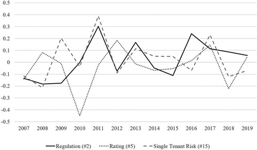
We observe that topic #2 Regulation had decreased before/during the crisis and increased in the aftermath, representing strengthened regulatory requirements after the crisis. Contrary, Single Tenant Risk (#15) peaked in 2009 and 2011 and has increased on average in the aftermath of the subprime crisis. This might be due to strengthened disclosure requirements, or it showcases that risk factors become immanent or even real threats for the company during an economic crisis. Rating (#5) dropped in the year 2010 and has oscillated since then around zero. This trend may reflect the loss of confidence in rating agencies following the events of 2007 and 2008. In summary, probabilities of appearance are time-varying and deviate from their previous level when specific events (e.g. subprime crisis) occur. Thus, disclosure frequencies reflect changes in firms’ reporting behavior caused by specific events, confirming the validity of the STM.

5.8. Generalization of the results with another dataset

In order to test the theoretical-motivated findings that STM is superior in comparison to CTM and LDA in analyzing risk, we repeat the major empirical analyses of Subsections 5.1. and 5.6. to a new dataset – mortgage REITs and unclassified REITs. Mortgage REITs, unlike equity REITs, exhibit less homogeneity, a diminished perception among investors, and lower quality and standardization in risk reporting. Our findings for this new sample support our previous findings. Notably, the STM algorithm yields more meaningful and statistically significant topics explaining the return’s volatilities compared to the other two algorithms (CTM and LDA). The risk factor’s coefficients are mostly negative supporting the risk reduction argument through corporate disclosures (convergence argument). The coefficient’s magnitudes reduce over the horizon (Model 1 to Model 3). Most of the controls are insignificant or have a higher influence in the long run. These findings align with the efficient market hypothesis, suggesting that the impact of new information (risk topics) diminishes and the impact of fundamentals increases as time progresses. The two alternative textual variables ($\mathrm{Text}\mathrm{\_Length}$ and $\mathrm{FOG}$) are never significant so the STM-derived risk topics convey the information. Consequently, these alternatives are not suitable as viable alternatives for the risk topics. The goodness of fit (R²) decreases from STM to CTM and to LDA supporting that STM-based risk factors are most suitable to explain the return volatility. The descriptive statistics of the new variables and the regression results are presented in Table D.1 and D.2 in Appendix D.

Considering the unfavorable market condition in this new dataset, we have reasons to conclude that our results can be generalized and the unsupervised machine-learning algorithm incorporating metadata of pre-specified covariates (STM) produces more meaningful and statistically significant topics influencing volatility compared to the other two ML algorithms or straightforward risk factors.

6. Conclusion

Firms have to inform their shareholders about the expected implications and consequences of adverse events so that the investors are able to monitor the current and future risk factors a firm is facing and integrate them into their decision-making analysis. Specifically, the SEC mandates firms to discuss the most relevant factors that may entail speculative or risky aspects for the firm in their 10-Ks.

Recognizing the temporal and cognitive limitation of human investors to read and react to the massive amount of text, we exploit unsupervised machine learning approaches (STM, CTM, and LDA), allowing the user to identify and quantify the risk factors discussed in REITs’ 10-Ks. However, since the so-far most used LDA is limited when identifying common risk factors across industries or sectors, we extend the applied toolbox with the advanced topic modeling approaches (STM and CTM) and are the first who apply these techniques in the accounting and finance domain. We are able to confirm the theoretical and previously shown superiority of STM over CTM and LDA in an economic application.

To assess whether our machine-assisted topic modeling presents a valid approach to quantify risk in narrative form, we analyze whether the STM extracted risk factors help to explain the perceived risk on the stock market in general. In a first step, we observe that models incorporating topic probabilities contribute to a more detailed understanding of how a firm's volatility can be explained, particularly in the short term. Simple straight-forwarded proxies of textual variables (e.g. word count, text length) are not viable alternatives for topic-modeling derived risk topics. In the next step, we find that the majority of risk topics are significantly associated with volatility, confirming the effectiveness of our model in comparison to LDA-focused studies which find for example mostly insignificant results (Bao and Datta 2014). Furthermore, we allow our fine-grained risk topics to carry all three types of risk perception (null argument, divergence argument, and convergence argument, see Kravet and Muslu 2013). This helps us to resolve contradicting results in the literature by our way of addressing a problem.

We find evidence supporting all three types of price reactions to information. Four risk factors support the null argument of uninformative disclosures, three risk factors reveal previously unknown contingencies to investors, thus increasing their risk perceptions (divergence argument), and the majority (nine risk factors) decrease risk perceptions (convergence argument). We repeat our primary analyses using new data under unfavorable market conditions to generalize our outcomes. The results from the new data also substantiate our key findings. The predominance of risk-reducing risk factors is in line with the majority of the previous literature using more straight-forwarded measures. In addition to previously used method of measuring qualitative textual information by counting words, we can combine this idea of an impact by quantity with our measure of probability. This hybrid model – combining machine learning with the word-counting factor – confirms our previous finding and explains best the variations within our dataset. This achieved finding would not be possible by the so-far mostly used approaches. Thus, we conclude that a combination of the classical word count and our machine-assisted topic modeling helps to explain investor risk perceptions most efficiently. This is our contribution from the technical part.

From the practical part, we contribute the finding that Item 1A in the 10-K filings primarily provides essential information on risk factors resolving uncertainties instead of disclosing new risk factors. Consequently, it seems like executives’ concerns of adverse effects of disclosing ‘negative’ information are baseless and risks described in 10-Ks can indeed be considered ‘good news’ as long as executives clarify the implications of already known risk.

Our findings support the pursuit to reduce information asymmetry by regulators (e.g. SEC) since both firms and shareholders benefit from reduced volatility showing that markets efficiently incorporate information into prices. In addition, our idea combining machine learning/topic modeling with a classical and straight-forwarded word-counting method as well as state-of-the-art econometric models may help to pave the way for more applications of natural language processing since previous methods were not able to give a deeper understanding of whether and which risk topics influence investors’ risk perception.

Acknowledgements

The authors wish to thank Thies Lindenthal, Masaki Mori, McKay Price, Erik Devos, Erkan Yönder, and the participants of the AREUEA-ASSA Conference 2021, Cambridge Real Estate Seminar 2021, ARES and ERES Meeting 2021, and the AREUEA International Conference 2021 for their insightful comments and suggestions on earlier versions of this paper. This paper circulated previously under the title: ‘Can Risks be Good News? Revealing Risk Perception of Real Estate Investors using Machine Learning’.

Disclosure statement

No potential conflict of interest was reported by the author(s).

Additional information

Notes on contributors

Marina Koelbl

Marina Koelbl received her doctorate from the IREBS International Real Estate Business School/University of Regensburg on the topic of Textual Analysis of Corporate Disclosures: The Case of REITs. Since then, she is working in the industry for a real estate development company.

Ralf Laschinger

Ralf Laschinger is a PhD student in the Department of Finance at the University of Regensburg. His doctoral research focuses on various topics in machine learning and FinTech.

Bertram I. Steininger

Bertram I. Steininger is an Associate Professor of Real Estate and Finance at the Department of Real Estate and Construction Management. He is affiliated with the cross-disciplinary research center Digital Futures (KTH, SU, and RISE). His research encompasses a wide range of topics within real estate and finance, including artificial intelligence (AI), machine learning (ML), FinTech/PropTech, tokenization, natural risk, sustainability, and direct and indirect investment vehicles (REIT, REOC, funds, crowdfunding).

His research has received funding from industry, private, and public organizations. He is an editor for several field journals and serves as an advisor for start-ups. Additionally, he frequently delivers scientific talks and participates in panel discussions. His work has been published in leading journals such as the Journal of Banking and Finance, Journal of Portfolio Management, Journal of Business Ethics, European Journal of Finance, Journal of Financial Research, Journal of Business Economics, Journal of Real Estate Finance and Economics, Journal of Housing Research, Journal of Property Investment & Finance, and Journal of Real Estate Portfolio Management.

Wolfgang Schaefers

Wolfgang Schaefers is a Professor of Real Estate Management. Since 2004, Dr. Schaefers has both taught and researched as a Full Professor and Head of the Chair of Real Estate Management at the IREBS International Real Estate Business School/University of Regensburg.

His main areas of research include Real Estate Asset Pricing, Big Data Analytics in Real Estate, Leadership Topics in Real Estate, and Infrastructures as an Asset Class. He frequently publishes textbooks in real estate and academic articles in leading journals (i.e. Journal of Real Estate Finance and Economics, Journal of Real Estate Research, Journal of Property Research, Journal of European Real Estate Research, German Journal of Real Estate Research).

Notes

1 This paper provides only an overview of (LDA and CTM); for deeper insights, we refer to the original papers by Blei, Ng, and Jordan (2003), Blei and Lafferty (2007).

2 To apply topic models, we use the programming language R (version 4.0.2) and the corresponding packages topicmodels and STM, authored by Grün and Hornik (2011) and Roberts, Stewart, and Tingley (2019); we use the edgarWebR package for parsing.

3 Actually, there is a second risk section in the 10-K. Item 7A lists “quantitative and qualitative disclosures about market risk” which are relevant for a company (e.g. interest rate risk or foreign currency exchange risk). However, Item 7A differs from Item 1A in that this section not only names but additionally quantifies the impact of the individual risk factors on future firm performance. Thus, managers usually use numbers to describe how risk factors affect firms’ filings in this section. Additionally, with an average length of only 6,680 words, Item 7A is just a tenth of the average length of Item 1A. Given that our method focuses on textual data, i.e. the words used to qualitatively describe relevant risks, we exclude Item 7A from the main analyses. This is essential because topic models cannot take numbers into account and shorter documents decrease the robustness of the topic model because it “learns” less from the data (Papilloud and Hinneburg 2018). However, for reasons of completeness, results for Item 7A are presented in Appendix D.

4 We additionally analyze the 10 and 20 trading-day periods. As expected, the results are in the intermediate ranges.

5 We describe the topic labels in the next subsection.

References

- Antweiler, W., and M. Z. Frank. 2004. “Is all That Talk Just Noise? The Information Content of Internet Stock Message Boards.” The Journal of Finance 59 (3): 1259–1294. https://doi.org/10.1111/j.1540-6261.2004.00662.x.
- Bamber, L., and Y. Cheon. 1995. “Differential Price and Volume Reactions to Accounting Earnings Announcements.” Accounting Review 70 (3): 417–441.
- Bao, Y., and A. Datta. 2014. “Simultaneously Discovering and Quantifying Risk Types from Textual Risk Disclosures.” Management Science 60 (6): 1371–1391. https://doi.org/10.1287/mnsc.2014.1930.
- Beyer, A., D. A. Cohen, T. Z. Lys, and B. R. Walther. 2010. “The Financial Reporting Environment: Review of the Recent Literature.” Journal of Accounting and Economics 50 (2-3): 296–343. https://doi.org/10.1016/j.jacceco.2010.10.003.
- Blei, D. M. 2012. “Probabilistic Topic Models.” Communications of the ACM 55 (4): 77–84. https://doi.org/10.1145/2133806.2133826.
- Blei, D. M., and J. D. Lafferty. 2007. “A Correlated Topic Model of Science.” Annals of Applied Statistics 1 (1): 17–35.
- Blei, D. M., A. Y. Ng, and M. I. Jordan. 2003. “Latent Dirichlet Allocation.” Journal of Machine Learning Research 3: 993–1022.
- Bond, S., and C. Xue. 2017. “The Cross Section of Expected Real Estate Returns: Insights from Investment-Based Asset Pricing.” The Journal of Real Estate Finance and Economics 54 (3): 403–428. https://doi.org/10.1007/s11146-016-9573-0.
- Buttimer, R. J., D. C. Hyland, and A. B. Sanders. 2005. “Real Estate REITs, IPO Waves and Long-Run Performance.” Real Estate Economics 33 (1): 51–87. https://doi.org/10.1111/j.1080-8620.2005.00112.x.
- Campbell, J. L., H. Chen, D. S. Dhaliwal, H. Lu, and L. B. Steele. 2014. “The Information Content of Mandatory Risk Factor Disclosures in Corporate Filings.” Review of Accounting Studies 19 (1): 396–455. https://doi.org/10.1007/s11142-013-9258-3.
- Chen, H., P. De, Y. Hu, and B. H. Hwang. 2014. “Wisdom of Crowds: The Value of Stock Opinions Transmitted Through Social Media.” Review of Financial Studies 27 (5): 1367–1403. https://doi.org/10.1093/rfs/hhu001.
- Chung, R., S. Fung, and S. Y. K. Hung. 2012. “Institutional Investors and Firm Efficiency of Real Estate Investment Trusts.” The Journal of Real Estate Finance and Economics 45 (1): 171–211. https://doi.org/10.1007/s11146-010-9253-4.
- Clayton, J., and G. MacKinnon. 2003. “The Relative Importance of Stock, Bond and Real Estate Factors in Explaining REIT Returns.” The Journal of Real Estate Finance and Economics 27 (1): 39–60. https://doi.org/10.1023/A:1023607412927.
- Cohen, L., C. Malloy, and Q. Nguyen. 2020. “Lazy Prices.” The Journal of Finance 75 (3): 1371–1415. https://doi.org/10.1111/jofi.12885.
- Cong, L. W., T. Liang, and X. Zhang. 2019. “Textual Factors: A Scalable, Interpretable, and Data-Driven Approach to Analyzing Unstructured Information. Interpretable, and Data-driven Approach to Analyzing Unstructured Information”. https://doi.org/10.2139/ssrn.3307057
- Cready, W. M. 2007. “Understanding Rational Expectations Models of Financial Markets: A Guide for the Analytically Challenged”. https://doi.org/10.2139/ssrn.999409.
- Danielsen, B. R., D. M. Harrison, R. A. Van Ness, and R. S. Warr. 2009. “REIT Auditor Fees and Financial Market Transparency.” Real Estate Economics 37 (3): 515–557. https://doi.org/10.1111/j.1540-6229.2009.00250.x.
- Das, S. R., and M. Y. Chen. 2007. “Yahoo! For Amazon: Sentiment Extraction from Small Talk on the web.” Management Science 53 (9): 1375–1388. https://doi.org/10.1287/mnsc.1070.0704.
- Das, S., M. Donini, M. Zafar, J. He, and K. Kenthapadi. 2022. “FinLex: An Effective use of Word Embeddings for Financial Lexicon Generation.” The Journal of Finance and Data Science 8: 1–11. https://doi.org/10.1016/j.jfds.2021.10.001.
- Devos, E., S. E. Ong, A. C. Spieler, and D. Tsang. 2013. “REIT Institutional Ownership Dynamics and the Financial Crisis.” The Journal of Real Estate Finance and Economics 47 (2): 266–288. https://doi.org/10.1007/s11146-012-9363-2.
- Doran, J. S., D. R. Peterson, and S. M. Price. 2012. “Earnings Conference Call Content and Stock Price: The Case of REITs.” The Journal of Real Estate Finance and Economics 45 (2): 402–434. https://doi.org/10.1007/s11146-010-9266-z.
- Fama, E. F. 1970. “Efficient Capital Markets: A Review of Theory and Empirical Work.” The Journal of Finance 25 (2): 383–417. https://doi.org/10.2307/2325486.
- Fama, E. F., and K. R. French. 1993. “Common Risk Factors in the Returns on Stocks and Bonds.” Journal of Financial Economics 33 (1): 3–56. https://doi.org/10.1016/0304-405X(93)90023-5.
- Feldman, R., S. Govindaraj, J. Livnat, and B. Segal. 2010. “Management’s Tone Change, Post Earnings Announcement Drift and Accruals.” Review of Accounting Studies 15 (4): 915–953. https://doi.org/10.1007/s11142-009-9111-x.
- Garcia, D. 2013. “Sentiment During Recessions.” The Journal of Finance 68 (3): 1267–1300. https://doi.org/10.1111/jofi.12027.
- Gaulin, M. 2019. “Risk Fact or Fiction: The Information Content of Risk Factor Disclosures”. Working Paper. Rice University.
- Glascock, J. L., C. Lu, and R. W. So. 2000. “Further Evidence on the Integration of REIT, Bond, and Stock Returns.” The Journal of Real Estate Finance and Economics 20 (2): 177–194. https://doi.org/10.1023/A:1007877321475.
- Grün, B., and K. Hornik. 2011. “Topicmodels: An R Package for Fitting Topic Models.” Journal of Statistical Software 40 (1): 1–30.
- Huang, K. W., and Z. L. Li. 2011. “A Multilabel Text Classification Algorithm for Labeling Risk Factors in SEC Form 10-K.” ACM Transactions on Management Information Systems 2 (3): 1–19. https://doi.org/10.1145/2019618.2019624.
- Israelsen, R. D. 2014. “Tell it Like it is: Disclosed Risks and Factor Portfolios”. https://doi.org/10.2139/ssrn.2504522.
- Jegadeesh, N., and D. Wu. 2013. “Word Power: A new Approach for Content Analysis.” Journal of Financial Economics 110 (3): 712–729. https://doi.org/10.1016/j.jfineco.2013.08.018.
- Karolyi, G. A., and A. Sanders. 1998. “The Variation of Economic Risk Premiums in Real Estate Returns.” The Journal of Real Estate Finance and Economics 17 (3): 245–262. https://doi.org/10.1023/A:1007776907309.
- Kelly, B., A. Manela, and A. Moreira. 2021. “Text Selection.” Journal of Business & Economic Statistics 39 (4): 859–879. https://doi.org/10.1080/07350015.2021.1947843.
- Kim, O., and R. E. Verrecchia. 1991. “Trading Volume and Price Reactions to Public Announcements.” Journal of Accounting Research 29 (2): 302–321. https://doi.org/10.2307/2491051.
- Kim, O., and R. E. Verrecchia. 1994. “Market Liquidity and Volume Around Earnings Announcements.” Journal of Accounting and Economics 17 (1-2): 41–67. https://doi.org/10.1016/0165-4101(94)90004-3.
- Koelbl, M. 2020. “Is the MD&A of US REITs Informative? A Textual Sentiment Study.” Journal of Property Investment and Finance 38 (3): 181–201. https://doi.org/10.1108/JPIF-12-2019-0149.
- Kravet, T., and V. Muslu. 2013. “Textual Risk Disclosures and Investors’ Risk Perceptions.” Review of Accounting Studies 18 (4): 1088–1122. https://doi.org/10.1007/s11142-013-9228-9.
- Kuhn, K. D. 2018. “Using Structural Topic Modeling to Identify Latent Topics and Trends in Aviation Incident Reports.” Transportation Research Part C: Emerging Technologies 87: 105–122. https://doi.org/10.1016/j.trc.2017.12.018.
- Lee, M.-L., M.-T. Lee, and K. C. H. Chiang. 2008. “Real Estate Risk Exposure of Equity Real Estate Investment Trusts.” The Journal of Real Estate Finance and Economics 36 (2): 165–181. https://doi.org/10.1007/s11146-007-9058-2
- Lehavy, R., F. Li, and K. Merkley. 2011. “The Effect of Annual Report Readability on Analyst Following and the Properties of Their Earnings Forecasts.” The Accounting Review 86 (3): 1087–1115. https://doi.org/10.2308/accr.00000043.
- Li, F. 2006. “Do Stock Market Investors Understand the Risk Sentiment of Corporate Annual Reports?” https://doi.org/10.2139/ssrn.898181.
- Li, F. 2008. “Annual Report Readability, Current Earnings, and Earnings Persistence.” Journal of Accounting and Economics 45 (2-3): 221–247. https://doi.org/10.1016/j.jacceco.2008.02.003.
- Li, F. 2010. “The Information Content of Forward- Looking Statements in Corporate Filings - A Naïve Bayesian Machine Learning Approach.” Journal of Accounting Research 48 (5): 1049–1102. https://doi.org/10.1111/j.1475-679X.2010.00382.x.
- Li, K., F. Mai, R. Shen, and X. Yan. 2021. “Measuring Corporate Culture Using Machine Learning.” The Review of Financial Studies 34 (7): 3265–3315. https://doi.org/10.1093/rfs/hhaa079.
- Ling, D., and M. Ryngaert. 1997. “Valuation Uncertainty, Institutional Involvement, and the Underpricing of IPOs: The Case of REITs.” Journal of Financial Economics 43 (3): 433–456. https://doi.org/10.1016/S0304-405X(96)00891-4.
- Lopez-Lira, A. 2023. “Risk Factors That Matter: Textual Analysis of Risk Disclosures for the Cross-Section of Returns.” https://doi.org/10.2139/ssrn.3313663.
- Loughran, T., and B. McDonald. 2011. “When is a Liability not a Liability? Textual Analysis, Dictionaries, and 10-Ks.” The Journal of Finance 66 (1): 35–65. https://doi.org/10.1111/j.1540-6261.2010.01625.x.
- Loughran, T., and B. McDonald. 2014. “Measuring Readability in Financial Disclosures.” The Journal of Finance 69 (4): 1643–1671. https://doi.org/10.1111/jofi.12162.
- Loughran, T., and B. McDonald. 2015. “The Use of Word Lists in Textual Analysis.” Journal of Behavioral Finance 16 (1): 1–11. https://doi.org/10.1080/15427560.2015.1000335.
- Miller, B. P. 2010. “The Effects of Reporting Complexity on Small and Large Investor Trading.” The Accounting Review 85 (6): 2107–2143. https://doi.org/10.2308/accr.00000001.
- Miller, M. H., and K. Rock. 1985. “Dividend Policy Under Asymmetric Information.” The Journal of Finance 40 (4): 1031–1051. https://doi.org/10.1111/j.1540-6261.1985.tb02362.x.
- Muslu, V., S. Radhakrishnan, K. R. Subramanyam, and D. Lim. 2015. “Forward-Looking MD&A Disclosures and the Information Environment.” Management Science 61 (5): 931–948. https://doi.org/10.1287/mnsc.2014.1921.
- Myers, S. C. 1984. “The Capital Structure Puzzle.” The Journal of Finance 39 (3): 574–592. https://doi.org/10.1111/j.1540-6261.1984.tb03646.x.
- Myers, S. C., and N. S. Majluf. 1984. “Corporate Financing and Investment Decisions When Firms Have Information That Investors Do Not Have.” Journal of Financial Economics 13 (2): 187–221. https://doi.org/10.1016/0304-405X(84)90023-0.
- Nelson, K. K., and A. C. Pritchard. 2016. “Carrot or Stick? The Shift from Voluntary to Mandatory Disclosure of Risk Factors.” Journal of Empirical Legal Studies 13 (2): 266–297. https://doi.org/10.1111/jels.12115.
- Ooi, J. T. L., J. Webb, and D. Zhou. 2007. “Extrapolation Theory and the Pricing of REIT Stocks.” Journal of Real Estate Research 29 (1): 27–56. https://doi.org/10.1080/10835547.2007.12091192.
- Papilloud, C., and A. Hinneburg. 2018. Qualitative Textanalyse Mit Topic-Modellen. Eine Einführung für Sozialwissenschaftler. Wiesbaden, Germany: Springer.
- Price, S. M., M. J. Seiler, and J. Shen. 2017. “Do Investors Infer Vocal Cues from CEOs During Quarterly REIT Conference Calls?” The Journal of Real Estate Finance and Economics 54 (4): 515–557. https://doi.org/10.1007/s11146-016-9557-0.
- Pritchard, J. K., M. Stephens, and P. Donnelly. 2000. “Inference of Population Structure Using Multilocus Genotype Data.” Genetics 155 (2): 945–959. https://doi.org/10.1093/genetics/155.2.945.
- Roberts, M., B. Stewart, and D. Tingley. 2019. “stm: R Package for Structural Topic Models.” Journal of Statistical Software 91 (2): 1–40. https://doi.org/10.18637/jss.v091.i02.
- Roberts, M. E., B. M. Stewart, D. Tingley, C. Lucas, J. Leder-Luis, S. K. Gadarian, B. Albertson, and D. G. Rand. 2014. “Structural Topic Models for Open-Ended Survey Responses.” American Journal of Political Science 58 (4): 1064–1082. https://doi.org/10.1111/ajps.12103.
- Ross, S. A. 1973. “The Economic Theory of Agency: The Principal’s Problem.” American Economic Review 63 (2): 134–139.
- Royston, J. P. 1982. “An Extension of Shapiro and Wilk’s W Test for Normality to Large Samples.” Applied Statistics 31 (2): 115–124. https://doi.org/10.2307/2347973.
- Schofield, A., and D. Mimno. 2016. “Comparing Apples to Apple: The Effects of Stemmers on Topic Models.” Transactions of the Association for Computational Linguistics 4: 287–300. https://doi.org/10.1162/tacl_a_00099.
- SEC. 2005. “Securities and Exchange Commission Final Rule, release no. 33–8591 (FR-75).” http://www. sec.gov/rules/final/33-8591.pdf.
- Tetlock, P. C. 2007. “Giving Content to Investor Sentiment: The Role of Media in the Stock Market." The Journal of Finance 62 (3): 1139–1168. https://doi.org/10.1111/j.1540-6261.2007.01232.x.
- Tetlock, P. C., M. Saar-Tsechansky, and S. Macskassy. 2008. “More Than Words: Quantifying Language to Measure Firms’ Fundamentals.” The Journal of Finance 63 (3): 1437–1467. https://doi.org/10.1111/j.1540-6261.2008.01362.x.
- Wooldridge, J. M. 2010. Econometric Analysis of Cross Section and Panel Data. 2nd ed. Cambridge, MA: MIT Press.