Portfolio optimization beyond utility maximization: the case of driftless markets

Abstract

This paper presents a novel perspective on portfolio optimization by recognizing that prices can be expressed as a scaled likelihood ratio of state price densities. This insight leads to the immediate conclusion that the optimal portfolio has a simple representation in terms of the likelihood ratio between the agent-defined physical measure and the risk-neutral measure, eliminating the need for utility maximization. The agent only needs to specify her choice of the physical measure, and we demonstrate both frequentist and Bayesian approaches for this selection. Utility maximization can be seen as a specific method for choosing the physical measure. The resulting likelihood ratio is log-utility optimal with respect to all benchmarks, aligning our approach with finding the growth optimal portfolio described in the literature. Notably, the expected log return corresponds to the relative entropy between the physical and risk-neutral measures, establishing a fundamental link to information theory. As a proof of concept, we explore previously unexplored territory in portfolio optimization, specifically addressing perceived mean reversion in specific driftless markets, such as foreign exchange (FX) markets.

Keywords:

• Likelihood ratio
• utility maximization
• relative entropy
• growth optimal portfolio
• Bayesian market

1. Introduction

1.1. Background and motivation

This paper introduces a novel perspective on optimal portfolio selection relevant to various market conditions, including driftless markets. Utilizing the change of numeraire theory as articulated by Geman, El Karoui, and Rochet (1995), our framework proposes that asset prices represent scaled likelihood ratios of their respective state price densities. This approach implies that the optimal portfolio price equals the ratio of the physical measure chosen by the investor to the market's risk-neutral measure, completely circumventing the conventional need for utility maximization. Within this framework, investors select their preferred physical measures to reflect their market outlooks. However, in incomplete markets, constructing such a portfolio may require identifying the nearest replicable alternative.

1.2. Advancements over traditional methods

Our methodology extends beyond the mean-variance framework established by Markowitz (1952). It fundamentally requires the specification of the state price density for each asset at time T as a key model input. This prerequisite enables a smooth transition to continuous time settings and is particularly effective with distributions that are infinitely divisible, such as the normal distribution. By focusing on state price densities, our approach permits a more sophisticated analysis that transcends the traditional emphasis on means and variances.

1.3. Theoretical foundations

Traditional asset pricing models predominantly focus on the stochastic evolution of asset prices. Theorem 2.1 demonstrates that specifying the state price density for a single asset is sufficient to deduce the densities for other assets. Closed-form solutions, like the geometric Brownian motion model posited by Merton (1971), calculate state price densities using asset volatility. However, in markets characterized by more complex dynamics, achieving unique or analytically expressible state price densities can be challenging. Moreover, models deviating from pure martingale structures may be incompatible with our theoretical framework, emphasizing the necessity to distinguish between pure and mixed martingale models.

1.4. Methodological innovations

Our approach is firmly rooted in statistical principles, requiring a precise definition of a likelihood function and treating state price densities as fundamental elements for price distribution modeling. Consistent with statistical theory, our model prioritizes state price densities as central components. Although our primary focus remains on normal distribution, the methodology is adaptable to any form of state price density, supporting a broad application across different financial markets.

1.5. Intrinsic optimality of logarithmic utility in state price density frameworks

Initially, traditional utility maximization techniques were considered for identifying optimal portfolios within a dynamic price evolution framework. However, in the context of foreign exchange markets, the feasibility of these solutions proved to be contingent on the choice of the benchmark currency – an undesirable dependency. For example, the optimal portfolio construction for an investor using Japanese Yen (JPY), involving assets denominated in Euro (EUR) and US Dollar (USD), should not be influenced by whether EUR or USD is chosen as the base currency.

Our analysis establishes that the logarithmic utility function uniquely provides a benchmark-independent portfolio configuration. Thus, the optimal portfolio's value corresponds to the likelihood ratio between the investor's physical measure and the reference asset's state price density. This finding reveals that the likelihood ratio intrinsically maximizes the logarithmic utility function. This property is inherent to the price structure itself and not merely a result of employing utility maximization strategies. This insight aligns with the notion of the growth optimal portfolio.

A critical finding of our study, formalized in Theorem 2.10, is that the growth optimal portfolio is the one replicable by a state price density that most closely approximates the physical measure. Specifically, any traded market asset X inherently constitutes a growth optimal portfolio with respect to its own state price density, denoted ${\mathbb{P}}^X$. Thus, an investor's choice of any asset as optimal is justified if their perspective concurs with the asset's state price density, emphasizing the alignment between individual investor views and market valuations.

1.6. Linking portfolio construction to information theory: expected log return as relative entropy

Portfolio optimizers that utilize various utility functions typically construct a portfolio V whose state price density ${\mathbb{P}}^V$ differs from the investor's belief ${\mathbb{P}}^M$ about the physical measure. The valuation of portfolio V, represented as the likelihood ratio between its state price density and the risk-neutral measure, inherently maximizes the logarithmic utility function. This maximization occurs regardless of the specific actions taken by the investor, ensuring that the investor invariably constructs a growth optimal portfolio in relation to its state price density.

The process of utility maximization can be understood as a method for selecting the state price density ${\mathbb{P}}^V$ of a preferred portfolio V. Once this density is established, further optimization becomes redundant, as the prices – expressed as scaled likelihood ratios–are already log-utility optimal. Investors may also choose to bypass traditional utility maximization by directly setting the state price density of their desired portfolio.

Furthermore, the expected log returns of these prices are equivalent to the expected log utility of the optimal payoff, aligning with the relative entropy between the two state price densities. Considering that relative entropy is a concept from information theory that measures information (as discussed by Shannon (1948)), these prices provide the most informative values concerning the divergence of state price densities among different assets. Consequently, the chosen physical measure fosters the creation of a growth optimal portfolio, aimed at maximizing expected log returns relative to all assets within the economy.

1.7. Statistical approaches: frequentist and Bayesian methods

Choosing the appropriate physical measure for financial modeling involves inherent subjectivity, often resolved through detailed statistical analysis. Our study juxtaposes frequentist and Bayesian methods in this selection process. In the frequentist paradigm, selection and validation of a model occur through hypothesis testing, leading to a statistically verifiable final price of a fund. The cornerstone of this approach is a hypothesis test that compares the likelihoods of the physical and risk-neutral measures using the Neyman-Pearson likelihood ratio test (Neyman and Pearson (1933)). This method fixes the model corresponding to the physical measure throughout the observation period, precluding any influence or modification by new data. Consequently, model selection in the frequentist approach may seem ad-hoc and lacks dynamic updates based on emerging data.

Conversely, the Bayesian approach considers a wide, potentially infinite array of models. It assesses the credibility of each model based on its posterior probability, which reflects the likelihood that a model is the most accurate given the observed data. This method conceptualizes a ‘fund of funds,’ where each subfund represents a different model parameter choice. The valuation of each subfund directly correlates with its model's posterior probability. Unlike the frequentist approach, Bayesian methods inherently accommodate dynamic updates. This dynamism stems from continuous refinements to posterior estimates as new data are integrated, thus dynamically adjusting the weighted consensus of these fixed likelihood functions.

1.8. Addressing parameter uncertainty in portfolio optimization

The specification of the physical measure in portfolio optimization introduces model risk, particularly when probabilistic models are estimated from limited historical data. As discussed by Kelly (1956) and Merton (1971), traditional methods often employ deterministic models that do not account for parameter uncertainty. Our study suggests that general utility maximization can mitigate this risk by aligning the parameters of an agent's physical measure with those of the risk-neutral measure.

1.9. Contributions to literature and methodological innovations

Historically, portfolio optimization literature has focused on markets characterized by drift. The concept of log utility maximization for discrete outcomes, originally put forth by Bernoulli in 1738 and revisited in his later work Bernoulli (1954), was later adapted into what is now known as the Kelly criterion (Kelly (1956)). This criterion provides a systematic approach to determine the optimal fraction of wealth to bet when the quoted odds diverge from an agent's own odds, aiming to maximize the expected geometric growth of the agent's wealth and thereby maximizing the entropy between subjective and market state price densities. The extension to multiple outcomes by Cover and Thomas (2012) further elaborates on this framework.

In settings involving geometric Brownian motion and varying utility functions, as seen in Merton (1971), the physical measure includes a drift parameter μ, differing from a driftless risk-neutral distribution. Despite this discrepancy in drift parameters, both measures are normally distributed with identical volatility σ. This scenario, known as Merton's portfolio problem, concludes that the log utility maximizer should invest a fraction $\frac{\mu }{{\sigma }^2}$ of their wealth in the risky asset. Our approach simplifies the solution to this problem using the likelihood ratio of prices, highlighting the effectiveness of our method. Additionally, we discuss how the risk aversion coefficient γ in the power utility function acts as a discount factor for drift, resulting in a drift parameter of $\frac{\mu }{\gamma }$ in the state price density of the power utility optimal portfolio. In scenarios where the physical measure exhibits no drift ($\mu =0$), and the agent concurs with the risk-neutral measure, full investment in the reference asset is optimal.

However, our focus extends beyond agreement on driftless mean parameters to differences in price process variability. Particularly in foreign exchange markets, many exchange rates display driftless and mean-reverting behavior with lower variability than that implied by the risk-neutral measure. This tendency leads to final prices clustering closer to the center of their respective confidence intervals. A notable example is pegged currencies, such as the EUR-DKK currency pair, which is constrained within a specific range of $[7.29252,7.62824]$ DKK for one EUR by design¹. This scenario falls outside the framework of Merton's portfolio problem, where the physical measure at a future time T exhibits less variability due to mean reverting price behavior, yet remains arbitrage-free as both physical and risk-neutral measures agree on spot volatility. We address this problem using the likelihood ratio of physical and risk-neutral measures, and the normal model's infinite divisibility aligns with the Brownian motion model, facilitating a replicable dynamic strategy.

1.10. Empirical analysis and practical implications

To illustrate the application of the frequentist approach in driftless markets, we model a physical measure with volatility scaled to eighty percent of that implied by the risk-neutral measure. The log utility optimal payoff corresponds to the scaled likelihood ratio of physical and risk-neutral densities. This framework facilitates statistical testing to accept or reject one of the two probability measures based on this likelihood ratio, with rejection regions corresponding to extreme price scenarios directly related to the concept of value at risk. In the context of a geometric Brownian motion model, we compute the value of this payoff at any intermediate time in a dynamic setting by taking the conditional expectation of the payoff. We then develop and validate a hedging strategy, demonstrating that the replicating portfolios closely align with theoretical predictions, particularly within the realm of foreign exchange rates. For empirical validation, we utilize exchange rate data from the European Central Bank, spanning from January 4, 1999 to December 29, 2023². This dataset encompasses 17 currencies, each with a complete observational history of T = 25 years relative to the EUR, which serves as the primary reference asset.

1.11. Bayesian approach and dynamic fund of funds

Our study also explores a Bayesian alternative to frequentist model selection by considering a spectrum of possible physical measures. This perspective leads to the creation of a fund consisting of subfunds, each representing an optimal payoff tied to a specific model of the physical measure. The initial allocation to each subfund reflects the prior distribution, embodying a subjective choice. In our analysis, we assume the scaling parameter follows a gamma distribution. As the study progresses, the final values of these subfunds adjust according to the posterior distributions, effectively demonstrating that more accurate models achieve higher realized profits. Despite each subfund operating under a frequentist framework–remaining static in its likelihood adjustments based on observed data–the overarching fund dynamically updates as the weight of each subfund evolves.

1.12. Empirical findings on mean reversion

In our empirical investigation using a volatility scaling factor of 0.8, we observe statistically significant mean reversion behavior in 9 out of 17 exchange rates relative to the EUR, at a 5% significance level. The currencies exhibiting this behavior include USD, JPY, DKK, PLN, AUD, CAD, HKD, KRW, and NZD. GBP, SEK, and NOK approach statistical significance, while CZK, CHF, HUF, and ZAR tend towards slight drifting behavior, with only CHF and ZAR reaching statistical significance.

1.13. Relation to existing literature

Significant advancements in determining the utility-maximizing agent's optimal payoff have been explored by Föllmer and Schied (2011), Karatzas and Shreve (1998), and Kramkov and Schachermayer (1999). More recently, Navratil, Taylor, and Vecer (2022) has demonstrated how to approximate this optimal payoff using a combination of traded options. Additionally, the theoretical relationship between the log-optimal portfolio and the numeraire portfolio is detailed in the continuous time framework by Becherer (2001) and in discrete time by Korn and Schäl (1999). These studies elucidate that if a numeraire portfolio exists, it must align with the log-optimal portfolio, thus providing a unified view of these fundamental portfolio strategies.

1.14. Robust utility maximization and Bayesian model averaging

The domain of robust utility maximization, which began with the seminal work of Gilboa and Schmeidler (1989) and expanded by Schied (2007) among others, addresses the challenges associated with fixed physical measures and uncertain volatility. This field has evolved to include methods similar to maximum likelihood estimation within a likelihood framework, showcasing the sophisticated methodologies employed in contemporary utility maximization. Furthermore, the recent work by Sass and Westphal (2021) incorporates filtering techniques in utility maximization, adeptly tackling the challenge of static physical measure updates. An alternative approach for managing model risk is Bayesian model averaging, as discussed by Al-Najjar and Weinstein (2015). This approach evaluates multiple models or hypotheses concurrently, each representing a different belief about the underlying probability distributions of outcomes. Models are weighted according to their Bayesian posterior probabilities, updated as new information is obtained, thus averaging over Knightian uncertainty and recognizing the existence of multiple potential ‘true’ models.

1.15. State price densities and asset pricing

The representation of prices as likelihood ratios of state price densities draws from the change of numeraire theory introduced by Geman, El Karoui, and Rochet (1995) and extended by Vecer (2011). This theory connects two numeraire measures with the Radon-Nikodym derivative as the scaled price. The prevailing asset pricing approach first specifies the price process's evolution and identifies the martingale pricing measure. However, this approach can be limited as the price evolution itself may not suffice to uniquely identify the risk-neutral measure, especially in incomplete markets. In statistical theory, a model is characterized by its likelihood function, or the state price density for each individual asset. Operating without an initial state price density falls outside the modern statistical framework. Therefore, we commence with the specification of state price densities as the fundamental building blocks of the model, from which the evolution of the prices follow.

1.16. Historical context and mean-variance optimization

The mean-variance approach to portfolio optimization, introduced by Markowitz (1952), predates the utility-based approaches. This method is often seen as an approximation of log utility maximization by matching the first two moments of the distribution. While this approach consistently leads to analytical solutions and has a computational advantage over log utility maximization, it's important to note that in continuous time settings, the mean-variance approach may yield time-inconsistent solutions. The resulting optimal portfolio is static, contrasting sharply with the dynamic portfolio problems addressed by Merton. This approach's sensitivity to drift parameter estimation shares limitations with Merton's framework, where disagreements with the market primarily concern the drift parameter.

Black and Litterman (1992) propose adjustments in portfolio weights based on agents' predictions about future asset performance to address challenges in the practical application of the mean-variance method. Rockafellar and Uryasev (2000) introduce portfolio optimization using Conditional-Value-at-Risk as a risk measure, and DeMiguel, Garlappi, and Uppal (2009) show that uniform investment strategies, especially in high-uncertainty environments, can outperform traditional portfolio optimization methods. The robust optimization approach, particularly in response to the observations of DeMiguel, Garlappi, and Uppal (2009) regarding the 1/N-portfolio, has been further explored by Pflug, Pichler, and Wozabal (2012) and Sass and Westphal (2022). Their work demonstrates the asymptotic optimality of the 1/N-portfolio under increasing uncertainty, both in discrete and continuous time, providing a robust foundation for diversification strategies in uncertain market conditions. Lastly, the evolution of the Black and Litterman (1992) model with the integration of expert opinions in a continuous setting, as presented by Davis and Lleo (2021), marks a significant advancement in the field.

1.17. Contributions to foreign exchange (FX) markets

In the context of existing literature on risk premia in FX markets, our study introduces a unique approach. Da Fonseca and Dawui (2021) explores variance, semivariance, and semiskew risk premiums in currency markets using a model-free methodology based on currency options. Dierckx, Davis, and Schoutens (2022) demonstrate the use of machine learning to improve trading strategies that harvest the EUR/USD volatility risk premium. Additionally, the study of Fonseca et al. (2011) focuses on maximizing returns on foreign currency portfolios under worst-case exchange rate scenarios using robust optimization techniques. In contrast, our methodology emphasizes the scaled likelihood ratio of state price densities, a novel approach that particularly addresses driftless and mean-reverting behaviors in FX markets. This distinctive strategy positions our research as an innovative method for handling the volatility risk premium, offering an alternative perspective to traditional models and contributing to the broader understanding of risk management in currency trading.

1.18. Overview of paper structure

Our paper is structured as follows. Section 2 establishes the unique state price density implied by each market asset, interpreting portfolio optimization as a selection of the best statistical model. Section 3 discusses the uniqueness of the logarithmic utility function in numeraire invariance. Section 4 reconstructs Merton's optimal portfolio using elementary techniques and identifies the growth optimal portfolio in drifting markets. Section 5 extends these methods to driftless markets, specifically addressing foreign exchange rate variability. Section 6 incorporates the Bayesian approach by constructing a dynamic fund of funds, reflecting multiple distributional opinions, with performance dependent on the choice of initial endowments (priors).

2. Prices as likelihood ratios of state price densities

Let us begin with a fundamental observation: prices are likelihood ratios of their respective state price densities. This indicates that if the state price densities are specified, the price evolution is determined. Every investment-grade asset has its unique state price density. By linking an asset to its state price density, portfolio optimization can be seen as a method of selecting the most appropriate statistical model, based on the distribution of random market outcomes.

Consider an arbitrary asset Y, a fixed time T>0, and a finite set of outcomes Ω, also known as scenarios in finance. An Arrow-Debreu security (Arrow and Debreu 1954) is a contract to deliver a unit of asset Y in the scenario $\omega \in \mathrm{\Omega }$, and its corresponding price at time 0 is termed a state price. As buying all such contracts guarantees the delivery of one asset Y in the future, the prices of all Arrow-Debreu securities must sum to one, signifying that these prices can be interpreted as probabilities associated with the delivery of asset Y at a future time T. We denote the state price by $p\left(\omega |\hat{Y}\right)$, signifying that the state price depends on the underlying security $\hat{Y}$, a contract to deliver Y at a future time T.

In the context of investment-grade assets that lack time value, the future delivery contract of the asset is equivalent to the asset itself, denoted as $\hat{Y}=Y.$ In contrast, assets with inherent time value, such as currencies, often display a divergence between the future delivery contract (Y) and the asset itself. This discrepancy is exemplified in the comparison between a currency and its corresponding zero-coupon bond. For the sake of simplicity, our analysis will primarily focus on investment-grade assets. Within this scope, the pricing in relation to the currency is directly derived from discounting processes.

The concept of state price generalizes to the concept of state price density when the set of outcomes $\mathrm{\Omega }=\mathbb{R}$, such as in situations where the market scenarios ω represent continuous random variables, like the logarithmic return of prices. Using the notation ${\mathbb{P}}^Y:=p(\cdot |Y)$, we indicate the state price density corresponding to the reference asset Y. This notation aligns with Bayesian statistics, interpreting $p(\cdot |Y)$ as a likelihood function corresponding to an asset (or a model in a Bayesian sense) Y. This density, as defined, is unique, and other assets must have different density functions; otherwise, assets with the same density would be indistinguishable.

Let us introduce the following notation.

Definition 2.1

Price

Let $X_Y\left(t\right)$ denote the price of asset X in terms of the asset Y at time t: (1) $\text{1 unit of an asset }X=X_Y\left(t\right)\text{ units of an asset }Y.$(1)

The asset itself is not a number; therefore, the above equality should be understood in the sense of equivalence classes, meaning two assets are regarded as equal if they have the same price at a given moment. This notation has the advantage of keeping track of the underlying reference asset, which will be helpful in the following computations. For instance, ${\text{€}}_{\mathrm{\$}}\left(T\right)$ denotes how many dollars are needed to acquire one euro, and ${\mathrm{\$}}_{\text{€ }}\left(T\right)$ denotes how many euros are needed to acquire one dollar at time T.

An important property of the price used extensively in this paper is the Change of the Numeraire: (2) $V_Y\left(T\right)=V_X\left(T\right)\cdot X_Y\left(T\right).$(2) This follows immediately from Definition 2.1. Now, let us define the concept of derivative security.

Definition 2.2

Derivative Payoff

A derivative security V is a contract that pays off $V_Y(T,\omega )\ge 0$ units of an asset Y on the scenario ω at time T.

Proposition 2.3

The price of a derivative contract V at time 0 is given by (3) $V_Y\left(0\right)={\mathbb{E}}^Y\left[V_Y\right(T\left)\right].$(3)

Proof.

The representation of V at time zero is expressed as (4) $V\left(0\right)=\left[{\int }_{\mathrm{\Omega }}p\right(\omega |Y\left)V_Y\right(T,\omega \left)\mathrm{d}\omega \right]Y\left(0\right),$(4) or, in terms of the prices, (5) $V_Y\left(0\right)=\left[{\int }_{\mathrm{\Omega }}p\right(\omega |Y\left)V_Y\right(T,\omega \left)\mathrm{d}\omega \right]={\mathbb{E}}^Y\left[V_Y\right(T\left)\right].$(5)

It is important to note that we directly derive a martingale property for the prices, ensuring the absence of arbitrage. This is based on the condition that the price $V_Y\left(T\right)$ must either be a constant or satisfy the condition $p\left(V_Y\right(T)<V_Y(0\left)|Y\right)>0$. Additionally, specifying the state price density $p\left(\omega |Y\right)$ at a fixed future time T results in a pure martingale evolution for the prices.

Theorem 2.4

Prices as Likelihood Ratios

Given a fixed time T, the price of asset $X_Y\left(T\right)$ can be represented as the likelihood ratio of the respective state price densities corresponding to assets X and Y. Formally, this relationship is expressed as: (6) $X_Y(T,\omega )=\frac{p\left(\omega |X\right)}{p\left(\omega |Y\right)}\cdot X_Y\left(0\right)$(6) where this holds true under the condition that probability measure ${\mathbb{P}}^X$ is absolutely continuous with respect to ${\mathbb{P}}^Y$ (denoted as ${\mathbb{P}}^X\ll {\mathbb{P}}^Y$).

The concept of absolute continuity, denoted as ${\mathbb{P}}^X\ll {\mathbb{P}}^Y$, is fundamental in this theorem. It implies that for any event ω in the probability space Ω, if this event has a probability of zero under ${\mathbb{P}}^Y$, then it also has a probability of zero under ${\mathbb{P}}^X$. In practical terms, this ensures that all scenarios covered by ${\mathbb{P}}^X$ are also considered in ${\mathbb{P}}^Y$, making ${\mathbb{P}}^X$ a ‘finer’ measure relative to ${\mathbb{P}}^Y$. This requirement is crucial for the validity of the likelihood ratio formula, as it ensures that the division in the equation is well-defined and does not involve division by zero.

Proof.

An arbitrary derivative contract V admits two price representations depending on whether we benchmark it with respect to a reference asset Y or X: $V\left(0\right)={\mathbb{E}}^Y\left[V_Y\right(T\left)\right]\cdot Y\left(0\right)={\mathbb{E}}^X\left[V_X\right(T\left)\right]\cdot X\left(0\right).$Using the change of the numeraire formula, we can also write ${\mathbb{E}}^Y\left[V_Y\right(T\left)\right]\cdot Y\left(0\right)={\mathbb{E}}^Y\left[V_X\right(T)\cdot X_Y(T\left)\right]\cdot Y\left(0\right).$This means $\left[{\int }_{\mathrm{\Omega }}{V}_X\right(T,\omega )\cdot X_Y(T,\omega )\cdot p(\omega |Y\left)\mathrm{d}\omega \right]\cdot Y\left(0\right)=\left[{\int }_{\mathrm{\Omega }}{V}_X\right(T,\omega )\cdot p(\omega |X\left)\mathrm{d}\omega \right]X\left(0\right).$Since the integrals are equal for an arbitrary payoff function $V_X$, the integrands must be equal, giving $X_Y(T,\omega )\cdot p\left(\omega |Y\right)\cdot Y\left(0\right)=p\left(\omega |X\right)\cdot X\left(0\right),$which implies $X_Y(T,\omega )=\frac{p\left(\omega |X\right)}{p\left(\omega |Y\right)}{X}_Y\left(0\right).$

Theorem 2.1 is known in a different form from the theory of numeraire change, as introduced in Geman, El Karoui, and Rochet (1995), which determines the state price density ${\mathbb{P}}^X$ from the state price density ${\mathbb{P}}^Y$ via the Radon-Nikodym derivative being the scaled price: (7) $p\left(\omega |X\right)=\frac{X_Y(T,\omega )}{X_Y\left(0\right)}\cdot p\left(\omega |Y\right).$(7) This means that state price densities of assets follow from the evolution of the prices and knowledge of one state price density. This approach in asset pricing typically specifies the stochastic evolution of the price process, from which the state price density ${\mathbb{P}}^Y$ can be derived. However, complex price evolutions may not always lead to a uniquely identified state price density, as in the case of incomplete markets, or they may not have an analytical distribution, even in complete markets. In contrast, Theorem 2.1 treats the state price densities as known inputs from which the price distribution follows, aligning more closely with a statistical theory where the density, or likelihood function, is a fundamental model element. This perspective suggests starting with the specification of state price densities to derive the price model, where a likelihood ratio of any two densities can be a valid model of price evolution.

Note, this price representation is valid for a fixed time T, but can be extended to intermediate times. Certain infinitely divisible distributions (normal, Poisson, gamma) allow for continuous time evolution. While the same techniques can be applied for arbitrary state price density distributions, our focus remains on the normal model.

It is essential for ${\mathbb{P}}^X$ to be absolutely continuous with respect to ${\mathbb{P}}^Y$ to avoid division by zero in Equation (6(6) $X_Y(T,\omega )=\frac{p\left(\omega |X\right)}{p\left(\omega |Y\right)}\cdot X_Y\left(0\right)$(6) ). However, ${\mathbb{P}}^X$ and ${\mathbb{P}}^Y$ do not need to be equivalent, which is typical in scenarios like option contracts where asset X might expire worthless with positive probability from the perspective of another asset. The following remark underscores the martingale property of prices under an arbitrary numeraire measure.

Remark 2.5

Prices are Martingales Under Every Numeraire Measure

The price representation as the likelihood ratio implies that prices are expectations with respect to the state price density of each corresponding reference asset. For instance, (8) ${\mathbb{E}}^X\left[Y_X\right(T\left)\right]={\int }_{\mathrm{\Omega }}\frac{p\left(\omega |Y\right)}{p\left(\omega |X\right)}\cdot p\left(\omega |X\right)Y_X\left(0\right)\mathrm{d}\omega =Y_X\left(0\right),$(8) and the choice of the reference asset is arbitrary.

This implies that models with the state price density for each asset at a fixed time T lead to arbitrage-free martingale evolution with respect to all numeraires.

Note that any asset V available on the market generates a state price density $p\left(\omega |V\right)$. In particular, a derivative contract defined by its payoff at time T has the following density:

Proposition 2.6

Density Implied by a Derivative Payoff

Let V be a derivative payoff. Its state price density $p\left(\omega |V\right)$ is (9) $p\left(\omega |V\right)=\frac{V_Y(T,\omega )}{V_Y\left(0\right)}\cdot p\left(\omega |Y\right).$(9)

Proof.

Follows immediately from the price representation $V_Y(T,\omega )=\frac{p\left(\omega |V\right)}{p\left(\omega |Y\right)}\cdot V_Y\left(0\right).$

Let us determine the state price density of a portfolio P:

Proposition 2.7

State Price Density of a Portfolio

Consider a static portfolio P composed of assets $X^i$ (where $i=1,\dots ,N$) over the time interval $0\le t\le T$. The portfolio at time t is given by: (10) $P\left(t\right)=\sum _{i=1}^N{\mathrm{\Delta }}^i{X}^i\left(t\right),$(10) where ${\mathrm{\Delta }}^i\ge 0$ represents the quantity of asset $X^i$ in the portfolio, and each asset $X^i$ has a mutually equivalent state price density $p\left(\omega |X^i\right)$. The state price density of the portfolio P is given by: (11) $p\left(\omega |P\right)=\sum _{i=1}^N{w}^{i}p\left(\omega |X^i\right),$(11) where $w^i$ is the weight of asset $X^i$ in the portfolio P, calculated as: (12) $w^i={\mathrm{\Delta }}^i{X}_P^i\left(0\right),$(12) with the weights satisfying the constraint: (13) $\sum _{i=1}^N{w}^i=1.$(13)

Proof.

The state price density of the portfolio is $\begin{array}{rl}p\left(\omega |P\right)& =\frac{P_Y(T,\omega )}{P_Y\left(0\right)}\cdot p\left(\omega |Y\right)=\frac{\sum _{i=1}^N{\mathrm{\Delta }}^i{X}_Y^i(T,\omega )}{P_Y\left(0\right)}\cdot p\left(\omega |Y\right)\\ & =\frac{\sum _{i=1}^N{\mathrm{\Delta }}^i{X}_Y^i\left(0\right)\frac{p\left(\omega |X^i\right)}{p\left(\omega |Y\right)}}{P_Y\left(0\right)}\cdot p\left(\omega |Y\right)\\ & =\sum _{i=1}^N\left[{\mathrm{\Delta }}^i{X}_P^i\right(0\left)\right]p\left(\omega |X^i\right)=\sum _{i=1}^N{w}^{i}p\left(\omega |X^i\right),\end{array}$which is a linear combination of state price densities of the individual assets. The values $w^i$ represent the initial relative weights of asset i in the portfolio P with the property $\sum _{i=1}^N{w}^i=1$.

In this study, we delve into the concept of relative entropy, also known as the Kullback-Leibler divergence, a fundamental measure in information theory. Relative entropy quantifies how one probability distribution, $\mathbb{P}$, diverges from a second, reference probability distribution, $\mathbb{Q}$. While it provides a measure of the ‘distance’ between these two distributions, it is important to note that relative entropy is not a true distance in the mathematical sense, as it is not symmetric; the divergence of $\mathbb{P}$ from $\mathbb{Q}$ is generally not equal to the divergence of $\mathbb{Q}$ from $\mathbb{P}$. This asymmetry is often used to gauge the inefficiency of assuming that the true distribution is $\mathbb{Q}$ when it is actually $\mathbb{P}$. Additionally, the Kullback-Leibler divergence is always non-negative as a simple consequence of Jensen's inequality, which reflects the principle that there is always some ‘cost’ associated with using an approximation $\mathbb{Q}$ instead of the true distribution $\mathbb{P}$. The divergence from $\mathbb{Q}$ to $\mathbb{P}$ is defined as $D_{\mathrm{KL}}(\mathbb{P}\Vert \mathbb{Q})=\sum _{x}P\left(x\right)\log \left(\frac{P\left(x\right)}{Q\left(x\right)}\right)$ for discrete distributions, and by an analogous integral for continuous distributions.

Theorem 2.8

Expected Log Return is Relative Entropy

The expected logarithmic return of a price process is equivalent to the relative entropy between the state price densities of two assets. Formally, for assets X and Y and a fixed time T, this relationship is given by: (14) ${\mathbb{E}}^X[\log \left(\frac{X_Y\left(T\right)}{X_Y\left(0\right)}\right)]={\int }_{\mathrm{\Omega }}\log \left(\frac{p\left(\omega |X\right)}{p\left(\omega |Y\right)}\right)p\left(\omega |X\right)\mathrm{d}\omega =D_{\mathrm{KL}}({\mathbb{P}}^X\Vert {\mathbb{P}}^Y).$(14) Moreover, this relationship holds for any asset V in comparison to Y: (15) ${\mathbb{E}}^X[\log \left(\frac{X_Y\left(T\right)}{X_Y\left(0\right)}\right)]\ge {\mathbb{E}}^X[\log \left(\frac{V_Y\left(T\right)}{V_Y\left(0\right)}\right)]$(15) for any other asset V.

Proof.

Equation (14(14) ${\mathbb{E}}^X[\log \left(\frac{X_Y\left(T\right)}{X_Y\left(0\right)}\right)]={\int }_{\mathrm{\Omega }}\log \left(\frac{p\left(\omega |X\right)}{p\left(\omega |Y\right)}\right)p\left(\omega |X\right)\mathrm{d}\omega =D_{\mathrm{KL}}({\mathbb{P}}^X\Vert {\mathbb{P}}^Y).$(14) ) follows directly from Equation (6(6) $X_Y(T,\omega )=\frac{p\left(\omega |X\right)}{p\left(\omega |Y\right)}\cdot X_Y\left(0\right)$(6) ). Equation (15(15) ${\mathbb{E}}^X[\log \left(\frac{X_Y\left(T\right)}{X_Y\left(0\right)}\right)]\ge {\mathbb{E}}^X[\log \left(\frac{V_Y\left(T\right)}{V_Y\left(0\right)}\right)]$(15) ) is derived as follows: $\begin{array}{rl}{\mathbb{E}}^X[\log \left(\frac{V_Y\left(T\right)}{V_Y\left(0\right)}\right)]& ={\mathbb{E}}^X[\log \left(\frac{V_X\left(T\right)\cdot X_Y\left(T\right)}{V_Y\left(0\right)\cdot X_Y\left(0\right)}\right)]\\ & ={\mathbb{E}}^X[\log \left(\frac{X_Y\left(T\right)}{X_Y\left(0\right)}\right)]-{\mathbb{E}}^X[\log \left(\frac{X_V\left(T\right)}{X_V\left(0\right)}\right)]\\ & =D_{\mathrm{KL}}({\mathbb{P}}^X\Vert {\mathbb{P}}^Y)-D_{\mathrm{KL}}({\mathbb{P}}^X\Vert {\mathbb{P}}^V)\\ & \le D_{\mathrm{KL}}({\mathbb{P}}^X\Vert {\mathbb{P}}^Y)={\mathbb{E}}^X[\log \left(\frac{X_Y\left(T\right)}{X_Y\left(0\right)}\right)],\end{array}$using the change of numeraire formula $V_Y=V_X\cdot X_Y$.

Note that the choice of reference asset Y is arbitrary.

Given that Theorem 2.8 does not depend on the choice of the reference asset, we can define

Definition 2.9

Growth Optimal Portfolio

The portfolio V that maximizes the expected log return with respect to all numeraires under the physical measure $p\left(\omega |M\right)$ is called the growth optimal portfolio.

In particular, if we limit ourselves to the finite number of assets $X^i$, $i=1,\dots ,N$, and static portfolios over time horizon $[0,T]$ from Proposition 2.7, we get a major result of this paper that follows directly from Theorem 2.8:

Theorem 2.10

The growth optimal portfolio V with respect to the measure $p\left(\omega |M\right)$ is a static portfolio that minimizes (16) $D_{\mathrm{KL}}({\mathbb{P}}^M\Vert {\mathbb{P}}^V).$(16)

Proof.

Take Y as a reference asset. Then $\begin{array}{rl}{\mathbb{E}}^M[\log \left(\frac{V_Y\left(T\right)}{V_Y\left(0\right)}\right)]& ={\mathbb{E}}^M[\log \left(\frac{V_M\left(T\right)\cdot M_Y\left(T\right)}{V_M\left(0\right)\cdot M_Y\left(0\right)}\right)]\\ & ={\mathbb{E}}^M[\log \left(\frac{M_Y\left(T\right)}{M_Y\left(0\right)}\right)]-{\mathbb{E}}^M[\log \left(\frac{V_M\left(T\right)}{V_M\left(0\right)}\right)]\\ & =D_{\mathrm{KL}}({\mathbb{P}}^M\Vert {\mathbb{P}}^Y)-D_{\mathrm{KL}}({\mathbb{P}}^M\Vert {\mathbb{P}}^V).\end{array}$Thus $\underset{V}{max}{\mathbb{E}}^M[\log \left(\frac{V_Y\left(T\right)}{V_Y\left(0\right)}\right)]=D_{\mathrm{KL}}({\mathbb{P}}^M\Vert {\mathbb{P}}^Y)-\underset{V}{min}{D}_{\mathrm{KL}}({\mathbb{P}}^M\Vert {\mathbb{P}}^V).$The resulting optimal portfolio V is unique due to the convexity of the Kullback-Leibler divergence. It remains to be seen that the log return of this portfolio is maximized for all reference assets. Let X be an arbitrary numeraire, then ${\mathbb{E}}^M[\log \left(\frac{V_Y\left(T\right)}{V_Y\left(0\right)}\right)]=D_{\mathrm{KL}}({\mathbb{P}}^M\Vert {\mathbb{P}}^X)-D_{\mathrm{KL}}({\mathbb{P}}^M\Vert {\mathbb{P}}^V),$which is also maximized for the smallest $D_{\mathrm{KL}}({\mathbb{P}}^M\Vert {\mathbb{P}}^V)$ as $D_{\mathrm{KL}}({\mathbb{P}}^M\Vert {\mathbb{P}}^X)$ is just a constant.

In particular, we have

Corollary 2.11

The asset X is the growth optimal portfolio under its state price density $p\left(\omega |X\right)$.

The growth optimal portfolio optimization identifies a replicable asset V with its state price density $p\left(\omega |V\right)=\sum _{i=1}^N{w}^{i}p\left(\omega |X^i\right)$. This density corresponds to a mixture distribution that is closest, in terms of relative entropy, to the agent's specified physical distribution $p\left(\omega |M\right)$. The process results in identifying optimal weights $w^i$, representing the proportion of wealth invested in each individual asset $X^i$, similar to the mean-variance procedure initiated by Markowitz (1952). The state price density $p\left(\omega |V\right)$ of the growth optimal portfolio V maximizes relative entropy compared to all benchmark assets, thereby earning the designation of a maximal entropy portfolio. Our Theorem 2.10 is anticipated to be applicable in a broader dynamic setting, provided specific technical conditions are defined to determine the set of replicable portfolios.

For binary random variables, the connection between expected log return and relative entropy was first noted by Kelly (1956). However, previous literature may not fully recognize that Theorem 2.8 applies to any general likelihood-based price model. In Section 4, we observe that Merton (1971) identified the growth optimal portfolio in drifting markets without explicitly making the connection to relative entropy.

An important implication of Theorem 2.10 is that an agent maximizing log utility and aligning with the state price density ${\mathbb{P}}^X$ of an asset X should invest entirely in that asset. If the asset is a portfolio, its state price density becomes the mixture distribution of the individual assets. Portfolio diversification thus involves selecting an appropriate mixture distribution, but this does not assure that the chosen distribution accurately reflects the true distribution.

In cases where an agent's density function $p\left(\omega |M\right)$ does not correspond to any market asset's state price density, complete markets allow for full replication of any payoff matching the agent's density. More complex scenarios arise in incomplete markets, where the agent must identify the closest replicable proxy density $p\left(\omega |V\right)$ from available assets.

Our study primarily focuses on the normal model, leading to geometric Brownian motion, which is a complete model. Therefore, any agent's specified physical measure can be perfectly replicated. We derive closed-form solutions for both the value function and the corresponding hedging strategy in a dynamic setting, demonstrating the practical applicability of our theoretical framework.

While our methodology could be expanded to more intricate models, our current focus serves as a proof of concept. This approach allows for direct comparison with the seminal work of Merton (1971), providing a concrete benchmark for assessing our methodology's effectiveness. We begin by examining price evolution, determining state price densities from the price dynamics inherent in the normal model. Alternatively, specifying state price densities first would dictate the subsequent price evolution, highlighting our method's flexibility in modeling and understanding price movements.

Example 2.12

Geometric Brownian Motion

Specification of the two state price densities ${\mathbb{P}}^X$ and ${\mathbb{P}}^Y$ in terms of two normal distributions leads to the geometric Brownian motion model. Let us derive these distributions from the traditional model of the stock price evolution: (17) $\mathrm{d}{X}_Y\left(t\right)=\sigma X_Y\left(t\right)\mathrm{d}{W}^Y\left(t\right).$(17) This gives a distributional opinion in terms of the reference asset Y, namely the simple return process $R\left(t\right)$: (18) $R\left(T\right)={\int }_0^T\frac{\mathrm{d}{X}_Y\left(t\right)}{X_Y\left(t\right)}=\sigma W^Y\left(T\right),$(18) which should be normally distributed $N(0,\sigma \sqrt{T})$ under ${\mathbb{P}}^Y$. To find the distributional opinion in terms of the reference asset X, we need to derive the dynamics of the inverse price $Y_X$: (19) $\mathrm{d}{Y}_X\left(t\right)=\mathrm{d}\left(\frac{1}{X_Y\left(t\right)}\right)=-\sigma Y_X\left(t\right)\mathrm{d}{W}^Y\left(t\right)+{\sigma }^2{Y}_X\left(t\right)\mathrm{d}t=\sigma Y_X\left(t\right)\mathrm{d}{W}^X\left(t\right)$(19) for a geometric Brownian motion $W^X\left(t\right)$ under measure ${\mathbb{P}}^X$ related to $W^Y\left(t\right)$ by: (20) $\mathrm{d}{W}^X\left(t\right)=-\mathrm{d}{W}^Y\left(t\right)+\sigma \mathrm{d}t.$(20) This implies that the simple return process: (21) $R\left(T\right)={\int }_0^T\frac{\mathrm{d}{X}_Y\left(t\right)}{X_Y\left(t\right)}=\sigma W^Y\left(T\right)=-\sigma W^X\left(T\right)+{\sigma }^{2}T$(21) is perceived as having a drift ${\sigma }^{2}T$ under measure ${\mathbb{P}}^X$. This is intuitively clear from Jensen's inequality; the inverse price process $Y_X$ is a result of a convex transformation $\frac{1}{x}$, and thus the convex operation on an undrifted process adds a positive drift. Thus, the simple return process has $N({\sigma }^{2}T,\sigma \sqrt{T})$ distribution under measure ${\mathbb{P}}^X$. The price $X_Y$ follows the likelihood ratio of the two measures ${\mathbb{P}}^X$ and ${\mathbb{P}}^Y$, specifically: (22) $\begin{array}{rl}{X}_Y(T,x)& =\frac{p\left(x|X\right)}{p\left(x|Y\right)}\cdot X_Y\left(0\right)\\ & =\frac{\frac{1}{2\mathrm{\pi \sigma }\sqrt{T}}\cdot \exp (-\frac{(x-\sigma {)}^{2}T}{2{\sigma }^{2}T})}{\frac{1}{2\mathrm{\pi \sigma }\sqrt{T}}\cdot \exp (-\frac{x^2}{2{\sigma }^{2}T})}\cdot X_Y\left(0\right)\\ & =\exp (x-\frac{1}{2}{\sigma }^{2}T)\cdot X_Y\left(0\right),\end{array}$(22) where x is a random variable with a $N(0,\sigma \sqrt{T})$ distribution under measure ${\mathbb{P}}^Y$. Note that the distributional opinions are: (23) ${\mathbb{P}}^X:R\left(T\right)\sim N({\sigma }^{2}T,\sigma \sqrt{T}),{\mathbb{P}}^Y:R\left(T\right)\sim N(0,\sigma \sqrt{T}).$(23) These are not the only possible choices leading to the same geometric Brownian motion model. We obtain the same distribution if we focus on the log return process: (24) $\mathrm{d}\log \left(X_Y\right(t\left)\right)=\sigma \mathrm{d}{W}^Y\left(t\right)-\frac{1}{2}{\sigma }^2\mathrm{d}t=-\sigma \mathrm{d}{W}^X\left(t\right)+\frac{1}{2}{\sigma }^2\mathrm{d}t.$(24) The distributional opinions about this process are: (25) ${\mathbb{P}}^X:\log \left(\frac{X_Y\left(T\right)}{X_Y\left(0\right)}\right)\sim N(\frac{1}{2}{\sigma }^{2}T,\sigma \sqrt{T}),{\mathbb{P}}^Y:\log \left(\frac{X_Y\left(T\right)}{X_Y\left(0\right)}\right)\sim N(-\frac{1}{2}{\sigma }^{2}T,\sigma \sqrt{T}),$(25) giving: (26) $\begin{array}{rl}{X}_Y(T,x)& =\frac{p\left(x|X\right)}{p\left(x|Y\right)}\cdot X_Y\left(0\right)\\ & =\frac{\frac{1}{2\mathrm{\pi \sigma }\sqrt{T}}\cdot \exp (-\frac{(x-\frac{1}{2}\mathrm{\sigma T}{)}^2}{2{\sigma }^{2}T})}{\frac{1}{2\mathrm{\pi \sigma }\sqrt{T}}\cdot \exp (-\frac{(x+\frac{1}{2}\mathrm{\sigma T}{)}^2}{2{\sigma }^{2}T})}\cdot X_Y\left(0\right)=\exp \left(x\right)\cdot X_Y\left(0\right),\end{array}$(26) where x is a random variable with $N(-\frac{1}{2}{\sigma }^{2}T,\sigma \sqrt{T})$ distribution under measure ${\mathbb{P}}^Y$, which is the same as above.

3. State price density of utility maximizers

In the situation of multiple reference assets that each can be used as a riskless asset in the portfolio optimization, such as in the case of the foreign exchange market, it is desirable to obtain a portfolio that is invariant to the choice of the numeraire. We show that the only numeraire invariant utility function is the logarithmic function. The optimal payoff is the likelihood ratio of the agent's chosen measure and the state price density of the numeraire asset.

Proposition 3.1

State Price Density of Utility Maximizer

Consider a utility function $U\left(x\right)$ with $U^{\prime }\left(x\right)>0$, $U^{″}\left(x\right)<0$ defined only for positive wealth x>0. The state price density of portfolio V that maximizes ${\mathbb{E}}^M\left[U\right(V_Y\left(T\right)\left)\right]$ using the agent's state price density $p\left(\omega |M\right)$ is given by (27) $p\left(\omega |V\right)=\frac{I(\lambda \cdot \frac{p\left(\omega |Y\right)}{p\left(\omega |M\right)})p\left(\omega |Y\right)}{{\int }_{\mathrm{\Omega }}I(\lambda \cdot \frac{p\left(\omega |Y\right)}{p\left(\omega |M\right)})p\left(\omega |Y\right)\mathrm{d}\omega },$(27) where (28) $I\left(x\right)=\left[U^{\prime }\right(x){]}^{-1}$(28) and where λ is chosen so that (29) ${\int }_{\mathrm{\Omega }}I(\lambda \cdot \frac{p\left(\omega |Y\right)}{p\left(\omega |M\right)})p\left(\omega |Y\right)\mathrm{d}\omega =V_Y\left(0\right).$(29)

Proof.

This follows from a well-known result (for instance Kramkov and Schachermayer 1999 or Karatzas and Shreve 1998) that the random variable $V_Y\left(T\right)$ that maximizes (30) ${\mathbb{E}}^M\left[U\right(V_Y\left(T\right)\left)\right]$(30) is given by (31) $V_Y(T,\omega )=I(\lambda \cdot \frac{p\left(\omega |Y\right)}{p\left(\omega |M\right)}),$(31) where (32) $I\left(x\right)=\left[U^{\prime }\right(x){]}^{-1}$(32) and where λ is chosen so that (33) ${\int }_{\mathrm{\Omega }}I(\lambda \cdot \frac{p\left(\omega |Y\right)}{p\left(\omega |M\right)})p\left(\omega |Y\right)\mathrm{d}\omega =V_Y\left(0\right).$(33) The resulting density is (34) $p\left(\omega |V\right)=\frac{I(\lambda \cdot \frac{p\left(\omega |Y\right)}{p\left(\omega |M\right)})p\left(\omega |Y\right)}{{\int }_{\mathrm{\Omega }}I(\lambda \cdot \frac{p\left(\omega |Y\right)}{p\left(\omega |M\right)})p\left(\omega |Y\right)\mathrm{d}\omega },$(34) requiring that $I\left(x\right)\ge 0$, which is the case if we restrict ourselves to utilities defined only on positive wealth x>0.

Note that the condition $I\left(x\right)\ge 0$ is not satisfied for all utility functions (for example, exponential).

Equation (27(27) $p\left(\omega |V\right)=\frac{I(\lambda \cdot \frac{p\left(\omega |Y\right)}{p\left(\omega |M\right)})p\left(\omega |Y\right)}{{\int }_{\mathrm{\Omega }}I(\lambda \cdot \frac{p\left(\omega |Y\right)}{p\left(\omega |M\right)})p\left(\omega |Y\right)\mathrm{d}\omega },$(27) ) shows that the agent blends her opinion expressed in terms of the state price density $p\left(\omega |M\right)$ with the opinion of the reference asset expressed in terms of the state price density $p\left(\omega |Y\right)$. In general, this operation is numeraire dependent, and the resulting state price density $p\left(\omega |V\right)$ of this payoff disagrees with the agent's original density $p\left(\omega |M\right)$. The following Theorem identifies the case when the state price density $p\left(\omega |V\right)$ of the utility maximizer agrees with her subjective opinion $p\left(\omega |M\right)$.

Theorem 3.2

Numeraire Invariance of Log Utility

The only utility function that is numeraire invariant is $U\left(x\right)=C_1\log \left(C_{2}x\right)$ with the optimal payoff (35) $V_Y(T,\omega )=\frac{p\left(\omega |M\right)}{p\left(\omega |Y\right)}\cdot V_Y\left(0\right).$(35) The resulting expected optimal utility function is proportional to the expected log return, which equals the relative entropy (Kullback-Leibler divergence): (36) ${\mathbb{E}}^M[\log \left(\frac{V_Y\left(T\right)}{V_Y\left(0\right)}\right)]={\int }_{\mathrm{\Omega }}\log \left(\frac{p\left(x|M\right)}{p\left(x|Y\right)}\right)p\left(x|M\right)\mathrm{d}x=D_{\mathrm{KL}}({\mathbb{P}}^M\Vert {\mathbb{P}}^Y).$(36)

Proof.

In order for the resulting density $p\left(\omega |V\right)$ to be equal to the original density opinion $p\left(\omega |M\right)$, the function I must be in a form $I\left(x\right)=\frac{C}{x}$. This means $U^{\prime }\left(x\right)=\frac{C}{x}$, concluding that the resulting utility function is in the form (37) $U\left(x\right)=C_1\log \left(C_{2}x\right).$(37) The expected log return corresponds to the choice of constants $C_1=1$ and $C_2=\frac{1}{V_Y\left(0\right)}$.

4. Drifting markets

Let us illustrate our approach based on the fact that the price of a growth optimal portfolio corresponds to a simple likelihood ratio of the two state price densities on a problem of the drifting market that has been solved by using non-trivial methods of the stochastic optimal control. The utility maximizing mechanism works as the agent takes her opinion $p\left(\omega |M\right)$, chooses the utility function U and an asset Y that she considers as riskless, which the market interprets as an opinion $p\left(\omega |V\right)$ from Equation (27(27) $p\left(\omega |V\right)=\frac{I(\lambda \cdot \frac{p\left(\omega |Y\right)}{p\left(\omega |M\right)})p\left(\omega |Y\right)}{{\int }_{\mathrm{\Omega }}I(\lambda \cdot \frac{p\left(\omega |Y\right)}{p\left(\omega |M\right)})p\left(\omega |Y\right)\mathrm{d}\omega },$(27) ) that maximizes the log utility function. Let us apply this technique on a drifting market. Let us consider a geometric Brownian motion model for the $X_Y\left(t\right)$ price as (38) $\mathrm{d}{X}_Y\left(t\right)=\sigma X_Y\left(t\right)\mathrm{d}{W}^Y\left(t\right),$(38) meaning that the ${\mathbb{P}}^Y$ distribution opinion about the simple return process $R\left(T\right)$ defined by (39) $R\left(T\right)={\int }_0^T\frac{\mathrm{d}{X}_Y\left(t\right)}{X_Y\left(t\right)}=\sigma W^Y\left(T\right)$(39) is $N(0,\sigma \sqrt{T})$. The agent with a state price density ${\mathbb{P}}^M$ may believe that this return process is drifting with a drift rate μ. Thus, we have three state price densities to compare: (40) ${\mathbb{P}}^X:R\left(T\right)\sim N({\sigma }^{2}T,\sigma \sqrt{T}),{\mathbb{P}}^Y:R\left(T\right)\sim N(0,\sigma \sqrt{T}),{\mathbb{P}}^M:R\left(T\right)\sim N(\mathrm{\mu T},\sigma \sqrt{T}).$(40) The following result is known as Merton's portfolio problem, which states that a $\frac{\mu }{{\sigma }^2}$ fraction of wealth should be invested in the asset X.

Remark 4.1

Merton's Portfolio is Growth Optimal Portfolio

The growth optimal portfolio under density ${\mathbb{P}}^M=N(\mathrm{\mu T},\sigma \sqrt{T})$ of $R\left(T\right)$ is defined by the payoff that corresponds to the likelihood ratio (41) $\begin{array}{rl}{V}_Y(T,R(T\left)\right)& =\frac{N(\mathrm{\mu T},\sigma \sqrt{T})}{N(0,\sigma \sqrt{T})}{V}_Y\left(0\right)=\frac{\frac{1}{\sqrt{2\pi {\sigma }^{2}T}}\cdot \exp (-\frac{\left(R\right(T)-\mathrm{\mu T}{)}^2}{2{\sigma }^{2}T})}{\frac{1}{\sqrt{2\pi {\sigma }^{2}T}}\cdot \exp (-\frac{R(T{)}^2}{2{\sigma }^{2}T})}{V}_Y\left(0\right)\\ & =\exp \left(\frac{\mu }{{\sigma }^2}R\right(T)-\frac{1}{2}{\left(\frac{\mu }{\sigma }\right)}^{2}T)V_Y\left(0\right),\end{array}$(41) which is a well-known solution of Merton's portfolio problem. The stochastic evolution of this wealth process $V_Y(t,R(t\left)\right)$ as a function of the simple return process $R\left(t\right)$ is a ${\mathbb{P}}^Y$ martingale and thus, according to Ito's formula (42) $\begin{array}{rl}\mathrm{d}{V}_Y(t,R(t\left)\right)& =\frac{\mu }{{\sigma }^2}{V}_Y(t,R(t\left)\right)\mathrm{d}R\left(t\right)=\frac{\mu }{{\sigma }^2}\frac{V_Y(t,R(t\left)\right)}{X_Y\left(t\right)}\mathrm{d}{X}_Y\left(t\right)\\ & =\frac{\mu }{{\sigma }^2}{V}_X(t,R(t\left)\right)\mathrm{d}{X}_Y\left(t\right).\end{array}$(42) The entropy of this portfolio that corresponds to the expected log return is (43) ${\mathbb{E}}^M[\log \left(\frac{V_Y\left(T\right)}{V_Y\left(0\right)}\right)]=D_{\mathrm{KL}}({\mathbb{P}}^M\Vert {\mathbb{P}}^Y)=\frac{1}{2}{\left(\frac{\mu }{\sigma }\right)}^{2}T$(43) when benchmarked against the asset Y and (44) ${\mathbb{E}}^M[\log \left(\frac{V_X\left(T\right)}{V_X\left(0\right)}\right)]=D_{\mathrm{KL}}({\mathbb{P}}^M\Vert {\mathbb{P}}^X)=\frac{1}{2}{(\frac{\mu }{\sigma }-\sigma )}^{2}T$(44) when benchmarked against the asset X and these are the largest expected log returns the investor can get in the market.

As mentioned above, maximizers with the state price density ${\mathbb{P}}^M$ of any other utility functions produce the optimal payoff in the sense of the derivative security for which the market finds the equivalent state price density ${\mathbb{P}}^V$ that is log utility optimal: (45) $p\left(\omega |V\right)=\frac{I(\lambda \cdot \frac{p\left(\omega |Y\right)}{p\left(\omega |M\right)})p\left(\omega |Y\right)}{{\int }_{\mathrm{\Omega }}I(\lambda \cdot \frac{p\left(\omega |Y\right)}{p\left(\omega |M\right)})p\left(\omega |Y\right)\mathrm{d}\omega }.$(45) Let us illustrate this density transformation in the drift case when the agent uses $N(\mathrm{\mu T},\sigma \sqrt{T})$ together with the isoelastic (power) utility function (46) $U\left(x\right)=\frac{x^{1-\gamma }-1}{1-\gamma }$(46) for $\gamma >0$. Note that $\gamma \to 1$ corresponds to the logarithmic utility. This gives (47) $I\left(x\right)=x^{-\frac{1}{\gamma }}$(47) concluding that the transformed state price density is (48) $p\left(x|V\right)=\frac{{\left(\frac{p\left(x|M\right)}{p\left(x|Y\right)}\right)}^{\frac{1}{\gamma }}p\left(x|Y\right)}{\int {\left(\frac{p\left(u|M\right)}{p\left(u|M\right)}\right)}^{\frac{1}{\gamma }}p\left(u|Y\right)\mathrm{d}u}=N(\frac{\mu }{\gamma }T,\sigma \sqrt{T}).$(48) What it means is that an agent with a higher risk aversion $\gamma >1$ transforms her original opinion about the drift parameter μ by a factor γ, meaning that the resulting log utility equivalent state price density is distributionally closer to the density of the asset Y. The risk averse agent takes the distributional opinion of the reference asset ${\mathbb{P}}^Y$ as more authoritative than her own opinion ${\mathbb{P}}^M$. The portfolio that corresponds to the optimal payoff in Equation (31(31) $V_Y(T,\omega )=I(\lambda \cdot \frac{p\left(\omega |Y\right)}{p\left(\omega |M\right)}),$(31) ) is the growth optimal portfolio under the modified density in Equation (48(48) $p\left(x|V\right)=\frac{{\left(\frac{p\left(x|M\right)}{p\left(x|Y\right)}\right)}^{\frac{1}{\gamma }}p\left(x|Y\right)}{\int {\left(\frac{p\left(u|M\right)}{p\left(u|M\right)}\right)}^{\frac{1}{\gamma }}p\left(u|Y\right)\mathrm{d}u}=N(\frac{\mu }{\gamma }T,\sigma \sqrt{T}).$(48) ).

5. Driftless markets

Our approach to portfolio optimization, which focuses on identifying the growth optimal portfolio, proves effective even in scenarios where the agent and the risk-neutral measure concur on the absence of drift, but differ in their views on variability or the precise shape of the state price density. To our knowledge, this aspect of portfolio optimization has not been comprehensively explored in previous literature.

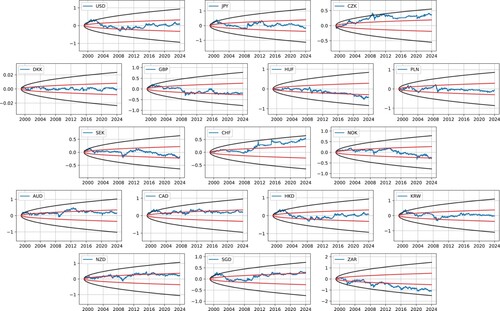
A primary point of divergence in our analysis concerns the final variability of asset prices. This is particularly evident in the foreign exchange market, where certain currency pairs display mean-reverting tendencies. For our study, we utilized data from the European Central Bank, focusing on currencies with a complete observational history spanning 25 years, from January 1999 to December 2023. This dataset includes 17 currencies: USD, JPY, CZK, DKK, GBP, HUF, PLN, SEK, CHF, NOK, AUD, CAD, HKD, KRW, NZD, SGD, and ZAR, benchmarked against the EUR.

In our analysis, we adopt the simplifying assumption that the observed exchange rates mirror the prices of corresponding bonds, which represent the risk-neutral densities. This assumption holds particularly when the interest rate differential between the two currencies involved is negligible. Figure 1 illustrates the log returns of the aforementioned currencies relative to the EUR, accompanied by confidence intervals that reflect the volatilities of these exchange rates. Notably, several currencies, such as USD, JPY, DKK, PLN, and HKD, show significant mean-reverting behavior. The DKK, a currency pegged to the EUR, presents a particularly interesting case. Conversely, other currencies like CZK and CHF have historically appreciated against the EUR, while currencies such as HUF and ZAR have shown a historical trend of depreciation.

Figure 1. Log returns of the exchange rates of selected currencies in terms of EUR, where the black region is 95% confidence interval and the red region is the 50% confidence interval as implied by the market volatility. Note that the log returns of most currencies stay in the tighter 50% confidence interval, indicating slight mean reversion. Several currencies exhibit a drift: CZK, HUF, CHF, and ZAR.

The agent may create an opinion that the markets may have a different (typically smaller) variability than implied by the daily moves of the market. Assuming a geometric Brownian motion model of the price process (49) $\mathrm{d}{X}_Y\left(t\right)={\sigma }_q{X}_Y\left(t\right)\mathrm{d}{W}^Y\left(t\right),$(49) the log return process $\log \left(X_Y\right(t\left)\right)$ evolves as (50) $\begin{array}{rl}\mathrm{dlog}\left(X_Y\right(t\left)\right)& =\frac{\mathrm{d}{X}_Y\left(t\right)}{X_Y\left(t\right)}-\frac{1}{2}{\left(\frac{\mathrm{d}{X}_Y\left(t\right)}{X_Y\left(t\right)}\right)}^2\\ & ={\sigma }_q\mathrm{d}{W}^Y\left(t\right)-\frac{1}{2}{\sigma }_q^2\mathrm{d}t\\ & =-{\sigma }_q\mathrm{d}{W}^X\left(t\right)+\frac{1}{2}{\sigma }_q^2\mathrm{d}t.\end{array}$(50) Thus, the log return process is slightly drifting from both perspectives of the two assets to ensure that the prices continue to evolve with the same dynamics. This rate is rather small; a typical currency pair volatility is on the scale of ${\sigma }_q=0.1$ with the corresponding annual drift rate being 0.005. However, this becomes measurable if observing this process over the time framework of several decades. The distributional opinions about the final value of the log return $\log \left(\frac{X_Y\left(T\right)}{X_Y\left(0\right)}\right)$ at time T from the perspective of the individual currencies X and Y are thus (51) ${\mathbb{P}}^Y:\log \left(\frac{X_Y\left(T\right)}{X_Y\left(0\right)}\right)\sim N(-\frac{1}{2}{\sigma }_q^{2}T,{\sigma }_q\sqrt{T}),{\mathbb{P}}^X:\log \left(\frac{X_Y\left(T\right)}{X_Y\left(0\right)}\right)\sim N(\frac{1}{2}{\sigma }_q^{2}T,{\sigma }_q\sqrt{T}).$(51) As the drift represents appreciation or depreciation of the currency pair regardless of the mean reversion, one may consider an equally weighted basket I of the two currencies as a benchmark with a distributional opinion (52) ${\mathbb{P}}^I:\log \left(\frac{X_Y\left(T\right)}{X_Y\left(0\right)}\right)\sim \frac{1}{2}N(-\frac{1}{2}{\sigma }_q^{2}T,{\sigma }_q\sqrt{T})+\frac{1}{2}N(\frac{1}{2}{\sigma }_q^{2}T,{\sigma }_q\sqrt{T})$(52) that is driftless.

In contrast to the log price evolution described by Equation (50(50) $\begin{array}{rl}\mathrm{dlog}\left(X_Y\right(t\left)\right)& =\frac{\mathrm{d}{X}_Y\left(t\right)}{X_Y\left(t\right)}-\frac{1}{2}{\left(\frac{\mathrm{d}{X}_Y\left(t\right)}{X_Y\left(t\right)}\right)}^2\\ & ={\sigma }_q\mathrm{d}{W}^Y\left(t\right)-\frac{1}{2}{\sigma }_q^2\mathrm{d}t\\ & =-{\sigma }_q\mathrm{d}{W}^X\left(t\right)+\frac{1}{2}{\sigma }_q^2\mathrm{d}t.\end{array}$(50) ), which follows a Brownian motion, an agent who believes in mean reversion would prefer the assumption: (53) $\mathrm{dlog}\left(X_Y\right(t\left)\right)=-\mathrm{\varphi log}\left(X_Y\right(t\left)\right)\mathrm{d}t+{\sigma }_q\mathrm{d}{W}^M\left(t\right).$(53) This represents a mean-reverting Ornstein-Uhlenbeck process, with $\varphi >0$. Its variance is given by: (54) ${\mathrm{Var}}^M(\log \left(\frac{X_Y\left(t\right)}{X_Y\left(0\right)}\right))=\frac{{\sigma }_q^2}{2\varphi }(1-e^{-2\mathrm{\varphi t}})\le {\sigma }_q^{2}t={\mathrm{Var}}^Y(\log \left(\frac{X_Y\left(t\right)}{X_Y\left(0\right)}\right)).$(54) This implies that the mean-reverting process exhibits smaller variance compared to a similar process without mean reversion, assuming the same spot volatility. As indicated in Equations (50(50) $\begin{array}{rl}\mathrm{dlog}\left(X_Y\right(t\left)\right)& =\frac{\mathrm{d}{X}_Y\left(t\right)}{X_Y\left(t\right)}-\frac{1}{2}{\left(\frac{\mathrm{d}{X}_Y\left(t\right)}{X_Y\left(t\right)}\right)}^2\\ & ={\sigma }_q\mathrm{d}{W}^Y\left(t\right)-\frac{1}{2}{\sigma }_q^2\mathrm{d}t\\ & =-{\sigma }_q\mathrm{d}{W}^X\left(t\right)+\frac{1}{2}{\sigma }_q^2\mathrm{d}t.\end{array}$(50) ) and (53(53) $\mathrm{dlog}\left(X_Y\right(t\left)\right)=-\mathrm{\varphi log}\left(X_Y\right(t\left)\right)\mathrm{d}t+{\sigma }_q\mathrm{d}{W}^M\left(t\right).$(53) ), both processes are driven by the same spot volatility. They agree on the parameter value but differ in the variability of the process for times t>0. This agreement on spot volatility prevents any potential arbitrage opportunities.

The parameter ϕ in the model is generally assumed to be constant. However, in reality, especially in the context of exchange rates, mean-reverting movements are often transient. Rather than making complex assumptions about the nature of ϕ, an agent might simplify the analysis by assuming that at a fixed future time T, the variance of the process $\log \left(X_Y\right(T\left)\right)$ will differ, represented as ${\sigma }_p^{2}T$.

In financial modeling, an agent's subjective belief about reduced variability in the log return process can be expressed as: (55) ${\mathbb{P}}^M:\log \left(\frac{X_Y\left(T\right)}{X_Y\left(0\right)}\right)\sim N(0,{\sigma }_p\sqrt{T})$(55) This expression holds true when ${\sigma }_p<{\sigma }_q$, indicating a belief in lower variability than the baseline. However, the framework is flexible and applicable for any ${\sigma }_p$ value, even if ${\sigma }_p>{\sigma }_q$. In practical applications, agents might consider the final standard deviation ${\sigma }_p\sqrt{T}$ to be a constant multiple, denoted by a, of the standard deviation ${\sigma }_q\sqrt{T}$ indicated by the risk-neutral density. Thus, we have: (56) ${\sigma }_p=a\cdot {\sigma }_q.$(56) It's important to note that the scaling factor a impacts the final variance, not the spot volatility, and the time factor T is eliminated when equating the variances. This assumption provides robustness, attributing any differences between expected and realized variances to the scaling parameter a. The agent must then form an opinion on the value of the shrinkage parameter a. Within the context of frequentist statistics, the choice of a is largely arbitrary. For the purposes of this discussion, we select a = 0.8. This indicates a belief in a 20% reduction in standard deviation compared to the baseline. However, the frequentist approach does not permit updating this parameter based on new data, which could be viewed as a limitation, especially in dynamic financial markets.

In contrast, the subsequent section on Bayesian portfolios outlines a more dynamic method. This approach involves establishing multiple funds, each defined by a different parameter value a. Although each individual fund operates with a fixed parameter a, the collective framework of the funds allows for dynamic updating. This update mechanism is influenced by the data-driven validation of the size of each fund. Such an approach results in an effective and statistically sound update process, aligning with Bayesian statistical principles, as opposed to the heuristic updating of the parameter a characteristic of the frequentist method.

Figure 2 illustrates the densities of various distributional opinions about the final value of the log return $\log \left(\frac{X_Y\left(T\right)}{X_Y\left(0\right)}\right)$. All three available assets, Y, X, and I, can serve as benchmarks, leading to slightly different payoffs. Here, we choose Y as EUR and X as the foreign currency.

Figure 2. Distributional opinions about the final value of the log return $\log \left(\frac{X_Y\left(T\right)}{X_Y\left(0\right)}\right)$ from the perspective of the two currencies ${\mathbb{P}}^X$ and ${\mathbb{P}}^Y$, their index ${\mathbb{P}}^I$, and the subjective agent's opinion ${\mathbb{P}}^M$ with parameters ${\sigma }_q=0.1$, ${\sigma }_p=0.08$, and T = 25.

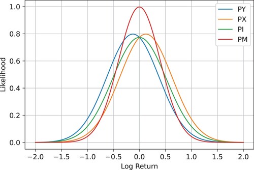
Figure 3 displays the corresponding likelihood ratios based on the distributional opinion of the final log return $\log \left(\frac{X_Y\left(T\right)}{X_Y\left(0\right)}\right)$. Values above 1 indicate profits, whereas values below 1 suggest losses. It is important to note that the range of potential profits varies with different benchmarks, and an upper limit exists to the maximum profit achievable. This limitation signifies that the extraction of potential discrepancies in the final variance is bounded. Conversely, the likelihood of a significant price drop is relatively low. Moreover, the agent has the potential to realize profits not only from the reduced variability of the underlying log return process but also from the appreciation or depreciation of the individual currency.

Figure 3. Likelihood ratios corresponding to the final log return $\log \left(\frac{X_Y\left(T\right)}{X_Y\left(0\right)}\right)$ of the subjective agent's opinion ${\mathbb{P}}^M$ against three available benchmarks: ${\mathbb{P}}^Y$, ${\mathbb{P}}^X$, and ${\mathbb{P}}^I$ from Figure 2 together with the rejection regions based on the Neyman-Pearson lemma. The central regions reject the state price density of the reference currency, the tail regions reject the state price density of the agent.

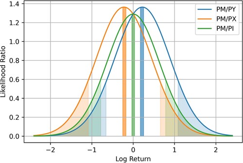
The optimal payoffs are represented as the likelihood ratio of two state price densities, which facilitates a direct statistical test to accept or reject a given density based on the Neyman-Pearson lemma. Considering two alternative hypotheses: (57) $H_0:\mathbb{P}={\mathbb{P}}^Y,H_1:\mathbb{P}={\mathbb{P}}^M,$(57) the hypothesis $H_0$ is rejected if $\frac{{\mathbb{P}}^M\left(x\right)}{{\mathbb{P}}^Y\left(x\right)}\ge C$, where C is a constant chosen such that the test's size is α: ${\mathbb{P}}^Y(\frac{{\mathbb{P}}^M\left(x\right)}{{\mathbb{P}}^Y\left(x\right)}\ge C)=\alpha$. As the prices are likelihood ratios, identifying the worst α fraction of price scenarios in terms of the value at risk corresponds to this testing approach.

However, it is worth noting that the value at risk is not an ideal measure of risk. In our portfolio optimization context, the rejection regions for the asset state price densities shown in Figure 3 are close but not overlapping. This implies that the observed data typically can reject at most one state price density. In the realm of frequentist statistics, this constitutes the most powerful test for hypothesis testing. The central regions of the figure reject the state price density of the reference asset, while the tail regions reject the state price density of the agent. The white regions denote acceptance of both alternatives as plausible.

Table 1 presents the results of a statistical test on the state price densities corresponding to the three considered benchmarks. The test statistics is the final value of the log return $\log \left(\frac{X_Y\left(T\right)}{X_Y\left(0\right)}\right)$. This test is against the agent's alternative hypothesis that the final price exhibits smaller variability and is conducted at a 5% significance level. The test employs the log return of the final exchange rate as the test statistic.

Table 1. Final log return $\log \left(\frac{X_Y\left(T\right)}{X_Y\left(0\right)}\right)$ as the test statistics of the exchange rate together with the rejection regions corresponding to all 3 different benchmarks. FX rates of currencies in bold stayed statistically significant around zero.

	LogR	Index	EUR	FX
USD	0.06	−[0.03, 0.03]	[0.16, 0.24]	[−0.24, −0.16]
JPY	−0.16	[−0.04, 0.04]	[0.25, 0.35]	[−0.35, −0.25]
CZK	0.35	[−0.02, 0.02]	[0.05, 0.09]	[−0.09, −0.05]
DKK	−0.00	[−0.00,0.00]	[−0.00, 0.00]	[−0.00,0.00]
GBP	−0.20	[−0.03, 0.03]	[0.11, 0.17]	[−0.17, −0.11]
HUF	−0.42	[−0.03,0.03]	[0.13, 0.20]	[−0.20, −0.13]
PLN	−0.06	[−0.03, 0.03]	[0.14, 0.21]	[−0.21, −0.14]
SEK	−0.16	[−0.02, 0.02]	[0.07, 0.12]	[−0.12, −0.07]
CHF	0.56	[−0.02, 0.02]	[0.07, 0.12]	[−0.12, −0.07]
NOK	−0.24	[−0.03, 0.03]	[0.11, 0.17]	[−0.17, −0.11]
AUD	0.16	[−0.03, 0.03]	[0.20, 0.28]	[−0.28, −0.20]
CAD	0.21	[−0.03, 0.03]	[0.17, 0.25]	[−0.25, −0.17]
HKD	0.06	[−0.03, 0.03]	[0.16,0.24]	[−0.24, −0.16]
KRW	−0.02	[−0.04, 0.04]	[0.23, 0.33]	[−0.33, −0.23]
NZD	0.24	[−0.04, 0.04]	[0.22, 0.31]	[−0.31, −0.22]
SGD	0.29	[−0.02, 0.02]	[0.10, 0.16]	[−0.16, −0.10]
ZAR	−1.08	[−0.05, 0.05]	[0.44, 0.60]	[−0.60, −0.44]

The findings reveal that, out of the 17 currencies, 9 exhibit statistical significance for the mean reversion behavior. This implies that for these currencies, either their state price density is rejected by the Neyman-Pearson test, or the final log return $\log \left(\frac{X_Y\left(T\right)}{X_Y\left(0\right)}\right)$ falls within the intermediate interval between two rejection regions. This observation is notably applicable for currencies such as USD, JPY, PLN, AUD, and HKD. The resulting payoff is deemed significant only when expressed in the benchmark corresponding to the statistically rejected currency.

An alternative test can be performed where the null hypothesis is the agent's subjective measure. In this scenario, the rejection region would be at the tails of the distribution. Specifically, the only two currencies that significantly moved to the tails are CHF (appreciating) and ZAR (depreciating). For CHF, the rejection regions are values above 0.46 (for CHF), 0.51 (for Index), and 0.65 (for EUR), indicating that the hypothesis of observing more central values is rejected (the observed log return is 0.56) by the state price densities corresponding to CHF and the Index. For ZAR, the rejection regions are values below $-2.05$ (for ZAR), $-1.17$ (for Index), and $-1.01$ (for EUR). This suggests that the hypothesis of observing more central values is rejected (the observed log return is $-1.08$) by the state price density corresponding to EUR, specifically when the optimal payoff is denominated in EUR.

Table 2 lists the optimal payoffs for a log utility maximizing agent across three available benchmarks, focusing on statistically significant payoffs. This table effectively highlights the complexities involved in portfolio optimization when dealing with multiple legitimate reference assets. Although the optimal portfolio remains the same across all benchmarks, the denomination in different currencies necessitates considering the final exchange rate between these currencies.

Table 2. Optimal values of the portfolios as a result of log utility maximization denominated in the index of two currencies, EUR, and the foreign currency.

	Index	EUR	FX
USD	1.280	1.321	1.239
JPY	1.281	1.181	1.380
CZK	0.826	0.970	0.683
DKK	1.250	1.249	1.250
GBP	1.192	1.073	1.312
HUF	0.998	0.791	1.204
PLN	1.274	1.233	1.315
SEK	1.188	1.094	1.282
CHF	0.595	0.756	0.433
NOK	1.161	1.023	1.299
AUD	1.263	1.364	1.161
CAD	1.230	1.356	1.103
HKD	1.281	1.317	1.245
KRW	1.299	1.283	1.316
NZD	1.237	1.384	1.089
SGD	1.089	1.247	0.930
ZAR	0.885	0.450	1.320

Note: Bold values indicate statistical significance. All statistically significant payoffs favor the hypothesis of smaller volatility with the exceptions of the CHF portfolio denominated in CHF and the Index and the ZAR portfolio denominated in EUR.

For example, consider the case of a fund denominated in ZAR (South African Rand). When this fund is valued in EUR (Euro), it experiences a statistically significant decrease in value. However, when the same fund is denominated in ZAR, it realizes a substantial profit. This scenario underscores the impact that currency denomination can have on the perceived success of an investment, highlighting a critical consideration for investors operating in international markets. While the resulting portfolio is optimal with respect to all available benchmarks, the exact specific choice depends on the agent's preference. In this respect, the EUR investor would consider the ZAR-EUR optimal portfolio quite substandard, but the ZAR investor could be satisfied with it.

Having the optimal payoff at the final time, the question is whether it can be dynamically priced at any intermediate time and whether the payoff can be replicated by a dynamic hedging strategy. For our analysis, it is sufficient to compute the optimal payoff with respect to one reference asset; let us take Y. It is also more convenient to translate the distributional discrepancy from the log return process $\log \left(X_Y\right(T\left)\right)$ to the simple return process $R\left(T\right)$ as the simple return process is used directly in hedging. The simple return process is only shifted from the log return process by a factor of $\frac{1}{2}{\sigma }_q^{2}T$ that follows from Equation (50(50) $\begin{array}{rl}\mathrm{dlog}\left(X_Y\right(t\left)\right)& =\frac{\mathrm{d}{X}_Y\left(t\right)}{X_Y\left(t\right)}-\frac{1}{2}{\left(\frac{\mathrm{d}{X}_Y\left(t\right)}{X_Y\left(t\right)}\right)}^2\\ & ={\sigma }_q\mathrm{d}{W}^Y\left(t\right)-\frac{1}{2}{\sigma }_q^2\mathrm{d}t\\ & =-{\sigma }_q\mathrm{d}{W}^X\left(t\right)+\frac{1}{2}{\sigma }_q^2\mathrm{d}t.\end{array}$(50) ). All other payoffs follow from the change of numeraire, meaning conversion by the exchange rate. The final optimal payoff in terms of the simple return process $R\left(T\right)$ is simply (58) $\begin{array}{rl}{V}_Y(T,R(T\left)\right)& =\frac{p\left(x|M\right)}{p\left(x|Y\right)}{V}_Y\left(0\right)=\frac{N(\frac{1}{2}{\sigma }_q^{2}T,{\sigma }_p\sqrt{T})}{N(0,{\sigma }_q\sqrt{T})}{V}_Y\left(0\right)\\ & =\frac{{\sigma }_q}{{\sigma }_p}\cdot \exp (-\frac{R(T{)}^2}{2T}(\frac{1}{{\sigma }_p^2}-\frac{1}{{\sigma }_q^2})+R(T)\cdot \frac{{\sigma }_q^2}{2{\sigma }_p^2}-\frac{1}{8}\frac{{\sigma }_q^{4}T}{{\sigma }_p^2}).\end{array}$(58)

Remark 5.1

Growth Optimal Portfolio

Following the previous discussion, the optimal portfolio V defined by the above payoff has the largest expected log return when benchmarked against any available asset X, Y, or I, where the expected log return corresponds to the relative entropy between the physical and the risk-neutral measures. In particular, the portfolio V maximizes expected log returns of prices $V_Y$, $V_X$, and $V_I$, satisfying ${\mathbb{E}}^M[\log (\frac{V_Y\left(T\right)}{V_Y\left(0\right)}\left)\right]=D_{\mathrm{KL}}({\mathbb{P}}^M\Vert {\mathbb{P}}^Y),$ ${\mathbb{E}}^M[\log (\frac{V_X\left(T\right)}{V_X\left(0\right)}\left)\right]=D_{\mathrm{KL}}({\mathbb{P}}^M\Vert {\mathbb{P}}^X)$, and ${\mathbb{E}}^M[\log (\frac{V_I\left(T\right)}{V_I\left(0\right)}\left)\right]=D_{\mathrm{KL}}({\mathbb{P}}^M\Vert {\mathbb{P}}^I)$ that follows from the price representation as the likelihood ratios and the numeraire invariance of the log utility function.

The following Theorem 5.2 provides the value of the optimal payoff at any time $t\in [0,T]$ along with its replicating portfolio.

Theorem 5.2

The value function v, representing the optimal wealth at time t, $V_Y\left(t\right)$, defined as (59) $v(t,x,{\sigma }_p,{\sigma }_q,T)={\mathbb{E}}^Y\left[\frac{N(\frac{1}{2}{\sigma }_q^{2}T,{\sigma }_p\sqrt{T})}{N(0,{\sigma }_q\sqrt{T})}|R\right(t)=x]V_Y\left(0\right)$(59) is given by (60) $v(t,x,{\sigma }_p,{\sigma }_q,T)={\sigma }_q\cdot \frac{\exp (-\frac{\frac{1}{4}{\sigma }_q^4\cdot t-{\sigma }_q^2\cdot x+(1-\frac{{\sigma }_p^2}{{\sigma }_q^2})\cdot x^2}{2\cdot ({\sigma }_p^2\cdot \frac{t}{T}+{\sigma }_q^2\cdot (1-\frac{t}{T}\left)\right)})}{\sqrt{{\sigma }_p^2\cdot \frac{t}{T}+{\sigma }_q^2\cdot (1-\frac{t}{T})}}\cdot V_Y\left(0\right)$(60) and the hedging position representing the number of units of the asset X at time t is (61) $\mathrm{\Delta }(t,x,{\sigma }_p,{\sigma }_q,T,X_Y(t\left)\right)=\frac{{\sigma }_q^{2}T+2\cdot ({\sigma }_p^2-{\sigma }_q^2)\frac{x}{{\sigma }_q^2}}{2\cdot ({\sigma }_p^{2}t+{\sigma }_q^2(T-t\left)\right)}\cdot \frac{v(t,x,{\sigma }_p,{\sigma }_q,T)}{X_Y\left(t\right)}.$(61)

Proof.

The value function is the conditional expectation of its payoff $V_Y\left(t\right)={\mathbb{E}}^Y\left[V_Y\right(T\left)|R\right(t\left)\right].$The conditional distribution of $R\left(T\right)$ is $N\left(R\right(t),{\sigma }_q\sqrt{T-t})$ and the formula follows from integration. The hedging position follows from Ito's formula: $\mathrm{d}v(t,R(t\left)\right)=\left[v_t\right(t,R\left(t\right)+\frac{1}{2}{\sigma }_q^2{v}_{\mathrm{rr}}(t,R(t\left)\right)]\mathrm{d}t+v_r(t,R(t\left)\right)\mathrm{d}R\left(t\right).$The $\mathrm{d}t$ term must be equal to zero (the process $v(t,R(t\left)\right)$ is a martingale). The evolution of the replicating portfolio P is $\mathrm{d}P\left(t\right)=\mathrm{\Delta }\left(t\right)\mathrm{d}{X}_Y\left(t\right)=\mathrm{\Delta }\left(t\right)X_Y\left(t\right)\mathrm{d}R\left(t\right).$Matching the $\mathrm{d}R\left(t\right)$ term in the evolution of the value function v and its replicating portfolio P, we get $\mathrm{\Delta }\left(t\right)X_Y\left(t\right)=v_r(t,R(t\left)\right),$concluding the proof.

Note that the sign of the hedging position depends mostly on the sign of the $({\sigma }_p^2-{\sigma }_q^2)R\left(t\right)$ term, which is quite intuitive. If the agent believes in a smaller final variance of the price, the term $({\sigma }_p^2-{\sigma }_q^2)$ is negative, and one should short when $R\left(t\right)>0$ and long when $R\left(t\right)<0$. In other words, one should be buying the currency that is currently under the original par. While this strategy is intuitive, for instance in the case of the pegged currency pair DKK-EUR, the exact hedging position is crucial, as any other position will not deliver the optimal payoff.

Figure 4 showcases the temporal evolution of the optimal portfolio, which is normalized to start at a value of 1, across a range of available currencies. This includes comparisons against the Euro (EUR), another unspecified currency, and the index composed of these two currencies. In our analysis, we employed an ad hoc scaling factor a = 0.8 in ${\sigma }_p=a\cdot {\sigma }_q$. It is important to note that other choices for the scaling factor are possible and could be explored in further studies. Notably, most of the portfolios under consideration generate profits, a finding that holds true even when these are benchmarked against all three selected reference assets.

Figure 4. The time evolution of the optimal value function for all currencies benchmarked with respect to EUR (blue graph), the other currency (orange graph), and the index of the two currencies (green graph). The choice of the scaling factor a in ${\sigma }_p=a\cdot {\sigma }_q$ is 0.8.

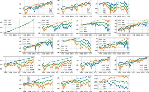
Figure 5 presents the progression of the theoretical value of the optimal payoff function, alongside its replicating portfolio. As the market does not offer the optimal value function for direct purchase, this value is replicated through active trading strategies aimed at securing it. This replication strategy is particularly noteworthy for its effectiveness over a 25-year horizon, even within the simplest normal model of the simple return process. This analysis assumes constant values for the volatility parameters, further underscoring the robustness of our approach in a simplified market scenario.

Figure 5. Comparison of the EUR theoretical optimal value function (blue) with its replicating portfolio (red).

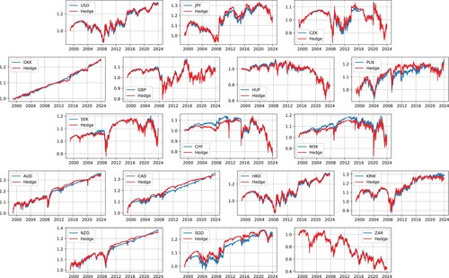
Table 3 presents the Sharpe ratios for these dynamically updated funds. Notably, the DKK case is distinct due to its currency peg to the EUR. For currencies that exhibit statistically significant mean reversion, the Sharpe ratios surpass 0.4. However, it's important to recognize that this represents a steady performance across a span of 25 years. Additionally, the relatively minor discrepancy between the variances indicates a constrained potential for gains, but concurrently, it suggests a limited risk of downside.

Table 3. Annualized Sharpe ratio.

	Index	EUR	FX
USD	0.454	0.241	0.180
JPY	0.542	0.159	0.214
CZK	−0.048	0.013	−0.078
DKK	0.906	0.906	0.894
GBP	0.214	0.075	0.337
HUF	0.023	−0.060	0.209
PLN	0.684	0.200	0.259
SEK	0.279	0.098	0.304
CHF	−0.198	−0.135	−0.221
NOK	0.200	0.046	0.268
AUD	0.314	0.422	0.113
CAD	0.250	0.710	0.089
HKD	0.456	0.237	0.185
KRW	0.551	0.196	0.208
NZD	0.276	0.419	0.083
SGD	0.108	0.318	−0.002
ZAR	−0.064	−0.149	0.264

Similar to the case of the portfolio performance from Table 2, the Sharpe ratio is dependent on the benchmarking asset. In extreme cases, the Sharpe ratio can be positive when a portfolio is benchmarked in one currency but negative when benchmarked in another due to the impact of exchange rate fluctuations. The primary driving force is the behavior of the exchange rate: if one currency is appreciating relative to the second currency, the returns benchmarked to the first, stronger currency will be lower, potentially turning positive returns benchmarked to the weaker currency into negative ones. This is notably the case with the ZAR-EUR exchange rate, where ZAR substantially depreciated with respect to EUR. Exchange rate volatility, which can also increase or decrease the standard deviation of returns, is a secondary factor. This behavior of a higher Sharpe ratio is visible when the optimal portfolio is benchmarked with respect to the index that leads to a smaller volatility for currency pairs that have negligible drifting behaviors, such as USD-EUR, JPY-EUR, PLN-EUR, HKD-EUR, or KRW-EUR. However, the impact of the different volatility alone cannot change the sign of the Sharpe ratio; it can only change its scale.

6. Bayesian portfolios

As previously mentioned, each state price density gives rise to a growth optimal portfolio, which maximizes the expected log return in comparison to any reference asset. One of the challenges with the frequentist approach, however, lies in its inherent rigidity regarding the selection of the likelihood function. This is evident in our model through the fixed choice of the parameter a. Frequentist statistics permits the consideration of various candidate models, selecting the one with the highest likelihood based on observed data, a process known as maximum likelihood estimation. However, a key issue with this approach is the practical difficulty in delivering a fund that aligns with this parameter. The corresponding replicating strategy would require dynamic adjustments to track the fund identified as the maximum likelihood estimator. Moreover, the fund deemed the best performer among model candidates, would necessitate an initial option premium.

In contrast, a Bayesian approach would involve constructing a linear combination of funds, where each is linked to a specific value of the parameter a. This method does not require an option premium and aligns with Bayesian statistics, which accommodates multiple values of the scaling factor a. This approach incorporates multiple densities and their likelihoods, offering a more flexible and potentially more practical solution.

In terms of a more general theory applicable to all models, we define a set of funds $V^{\theta }$, each corresponding to a choice of parameter $\theta \in \mathrm{\Theta }$ with the likelihood function $p\left(x|\theta \right)$. Here, Θ represents a set of parameters or models for the physical density.

Definition 6.1

Fund of Funds

A fund of funds I at time t is represented by (62) $I\left(t\right)={\int }_{\mathrm{\Theta }}{\mathrm{\Delta }}^{\theta }{V}^{\theta }\left(t\right)\mathrm{d}\theta ,$(62) where ${\mathrm{\Delta }}^{\theta }$ is a constant number of units of the fund $V^{\theta }.$

This representation is a linear combination of assets, and thus the fund of funds I possesses a state price density corresponding to the mixture distribution: (63) $p\left(x|I\right)={\int }_{\mathrm{\Theta }}\left[{\mathrm{\Delta }}^{\theta }{V}_I^{\theta }\right(0\left)\right]p\left(x|\theta \right)\mathrm{d}\theta .$(63) Derived from Proposition 2.7, the term $w^{\theta }\left(0\right)=\left[{\mathrm{\Delta }}^{\theta }{V}_I^{\theta }\right(0\left)\right]$ signifies the fraction of wealth invested in the fund $V^{\theta }$ at time t = 0 and is interpretable as a probability $p\left(\theta \right)$ of selecting the model $\theta \in \mathrm{\Theta }$. In financial terms, this represents the initial endowment of each fund. Statistically, this probability is known as a prior distribution. Since (64) $p\left(x|I\right)={\int }_{\mathrm{\Theta }}p\left(x|\theta \right)p\left(\theta \right)\mathrm{d}\theta =p\left(x\right),$(64) the conditional distribution of the fund of funds transitions into an unconditional distribution reflecting the cumulative opinion of the individual funds.

Theorem 6.2

Bayesian Portfolio

The fraction of wealth invested in the fund $V^{\theta }$ at time T, $w^{\theta }\left(T\right)=\left[{\mathrm{\Delta }}^{\theta }{V}_I^{\theta }\right(T\left)\right]$, is equivalent to the posterior distribution of θ given x: (65) $w^{\theta }\left(T\right)={\mathrm{\Delta }}^{\theta }{V}_I^{\theta }(T,x)=\frac{p\left(x|\theta \right)}{p\left(x|I\right)}{\mathrm{\Delta }}^{\theta }{V}_I^{\theta }\left(0\right)=\frac{p\left(x|\theta \right)\cdot p\left(\theta \right)}{p\left(x\right)}=p\left(\theta |x\right).$(65) The value of the fund of funds I, relative to the reference asset Y, is then given by: (66) $I_Y(T,x)={\int }_{\mathrm{\Theta }}{\mathrm{\Delta }}^{\theta }{V}_Y^{\theta }(T,x)\mathrm{d}\theta ={\int }_{\mathrm{\Theta }}{I}_Y\left(0\right)\cdot \frac{p\left(x\right)}{p\left(x|Y\right)}\cdot p\left(\theta |x\right)\mathrm{d}\theta =I_Y\left(0\right)\cdot \frac{p\left(x\right)}{p\left(x|Y\right)}.$(66)

This theorem highlights the Bayesian nature of the portfolio, where the final investment in each fund $V^{\theta }$ is determined by the posterior distribution $p\left(\theta |x\right)$. This approach allows for a dynamic adjustment of investments based on new information, reflected in the updating of the posterior probabilities. Thus, the fund of funds I becomes a flexible and adaptive portfolio, aligning with evolving market conditions and the investor's updated beliefs.

Applying this to the scaling factor a, the frequentist method typically involves selecting a single value based on historical observations, which can be arbitrary. To mitigate the risk of incorrect parameter selection, we propose diversifying the value of a by considering it as a random variable. This leads to the creation of infinitely many funds $V^a$, each corresponding to a unique choice of a. A natural choice for the distribution of initial endowment across these funds is a gamma distribution $\mathrm{\Gamma }(\alpha ,\text{β})$, defined by the density: (67) $p(x|\alpha ,\text{β})=\frac{{\text{β}}^{\alpha }}{\mathrm{\Gamma }\left(\alpha \right)}{x}^{\alpha -1}{e}^{-\text{β}x}.$(67) The mean μ and variance ${\sigma }^2$ of this distribution are given by: (68) $\mu =\frac{\alpha }{\text{β}},{\sigma }^2=\frac{\alpha }{{\text{β}}^2},$(68) establishing an inverse relationship: (69) $\alpha ={\left(\frac{\mu }{\sigma }\right)}^2,\text{β}=\frac{\mu }{{\sigma }^2}.$(69) In our example, we select $p\left(a\right)\sim \mathrm{\Gamma }(4,8)$, yielding a mean $\mu =0.5$ and standard deviation $\sigma =0.25$. Each choice of a corresponds to a fund $V^a$, with initial endowment proportional to the $\mathrm{\Gamma }(\alpha ,\text{β})$ density.

Figure 6 illustrates the performance of these individual funds with EUR as the reference asset. In the Bayesian investment approach, some funds may perform extremely poorly, even to the point of bankruptcy, but this risk is counterbalanced by the potential for other funds to perform exceptionally well. This trade-off is inherent in this approach. The value of the fund of funds I is computed as: (70) $I_Y\left(T\right)={\int }_0^{\mathrm{\infty }}{V}^a\left(T\right)p\left(a\right)\mathrm{d}a={\int }_0^{\mathrm{\infty }}{V}^a\left(T\right)\frac{{\text{β}}^{\alpha }}{\mathrm{\Gamma }\left(\alpha \right)}{a}^{\alpha -1}{e}^{-\text{β}a}\mathrm{d}a,$(70) represented by the red line in Figure 6. The performances of most Bayesian portfolios, listed in Table 4, surpass those from the frequentist framework in Table 2. This is attributed to the Bayesian portfolios being sampled from a distribution with a smaller mean scaling factor of 0.5, compared to the single choice of 0.8 in the frequentist approach. This lower mean scaling factor offers a higher potential for superior payoffs in scenarios with strong mean reverting behavior, but it also carries the risk of inferior performance when these expectations are not realized in practice.

Figure 6. The performance of individual funds as a function of the scaling parameter a for different currencies denominated in EUR. Currencies with smaller variability peak for values under a = 1. The red line corresponds to the mean performance of the funds sampled from the $\mathrm{\Gamma }(4,8)$ distribution for the scaling factor a.

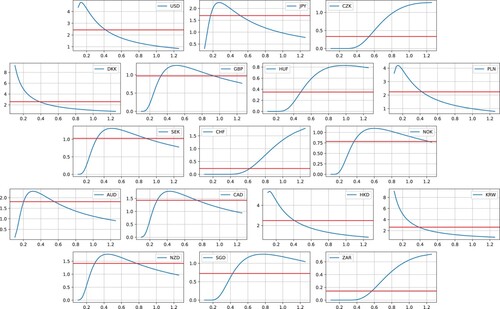
Table 4. Cumulative performance of the Bayesian portfolios.

	Index	EUR	FX
USD	2.360	2.436	2.284
JPY	1.840	1.697	1.984
CZK	0.285	0.335	0.236
DKK	2.585	2.585	2.586
GBP	1.079	0.971	1.187
HUF	0.440	0.349	0.531
PLN	2.314	2.240	2.388
SEK	1.114	1.026	1.202
CHF	0.178	0.227	0.130
NOK	0.890	0.784	0.996
AUD	1.677	1.812	1.543
CAD	1.296	1.429	1.162
HKD	2.422	2.490	2.354
KRW	2.669	2.636	2.702
NZD	1.266	1.417	1.116
SGD	0.632	0.724	0.541
ZAR	0.280	0.142	0.417

Figure 7 illustrates the temporal evolution of the posterior mean of a scaling parameter, computed using the following equation: (71) $a\left(t\right)={\int }_0^{\mathrm{\infty }}a\cdot p\left(a|R\right(t\left)\right)\mathrm{d}a$(71) In this context, the $\mathrm{\Gamma }(4,8)$ distribution is employed as the prior. This methodology represents a robust statistical approach for dynamically updating the scaling parameter a based on observed data, specifically the simple return process $R\left(t\right)$ at time t.

Figure 7. Temporal evolution of the mean posterior for the scaling factor parameter a.

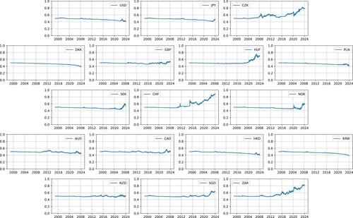
It is noteworthy that the posterior mean of the scaling parameter maintains relative stability. This stability is attributed primarily to the minor variance in distributional discrepancy, suggesting that a considerable duration might elapse before alternative values of the parameter become statistically significant.

Observations across various currencies indicate distinct trends. For drifting currencies such as the CZK, HUF, CHF, and ZAR, there is a discernible gradual increase in the scaling parameter. In contrast, for mean-reverting currencies like the USD, DKK, PLN, or KRW, a slight decrease in the scaling parameter is observed. These observations imply that the method effectively tracks temporal changes in the scaling parameter, exhibiting varying behaviors across different types of currencies.

This approach exemplifies the Bayesian philosophy in investing where diversification is achieved not only across assets but also across models (parameter choices), recognizing that while some investments may fail, others may yield substantial returns. This diversified strategy, represented by the fund of funds I, aims to balance the risk and potential rewards across a spectrum of scenarios defined by the scaling factor a.

7. Conclusion

In our research, we have applied an innovative methodology that circumvents traditional utility maximization, opting instead for a likelihood ratio representation of prices. This approach is specifically tailored to address the unique challenges of portfolio optimization in environments devoid of drift. A key insight of our method is the interpretation of prices as likelihood ratios, which establishes a crucial link between portfolio optimization and model selection within the domain of statistical theory.

Utilizing this perspective, our study successfully integrates both frequentist and Bayesian approaches, thereby offering comprehensive solutions to a wide array of portfolio selection problems. This innovative approach not only challenges the conventional methodologies in financial optimization but also bridges the theoretical gap between statistical theory and practical investment strategies, particularly in markets characterized by non-standard behaviors like the absence of drift.

Furthermore, we have discerned that the logarithmic function stands as the only utility function invariant under changes in the numeraire. This discovery implies that investors maximizing logarithmic utility are effectively maximizing their expected log return in comparison to all other assets. Notably, the expected utility in this context is synonymous with relative entropy, a key measure of information. This finding emphasizes the deep interconnection between portfolio optimization, utility theory, and information theory.

By converging these disciplines, our work lays out a comprehensive framework for understanding and implementing portfolio strategies, especially in scenarios where traditional market behavior assumptions, such as price drift, are not applicable. This multifaceted approach not only advances the theoretical understanding of portfolio optimization but also offers valuable practical insights for investors navigating complex financial markets. Through this synthesis, our research contributes significantly to the field, presenting new perspectives and tools for investors and theorists alike who are dealing with the challenges of modern financial environments.

Acknowledgments

Special thanks to Mete Soner, Ali Hirsa, and seminar participants at Columbia University and Stevens Institute of Technology for their valuable insights, which greatly enhanced this manuscript. Appreciation is also extended to anonymous referees for their meticulous reviews and constructive feedback on earlier drafts.

Data Availability Statement

The data that support the findings of this study are openly available in the European Central Bank repository at https://www.ecb.europa.eu/stats/eurofxref/eurofxref-hist.zip, derived from the European Central Bank Exchange Rate Data.

Disclosure statement

No potential conflict of interest was reported by the author(s).

Additional information

Funding

This work was partially supported by Grant Agency of the Czech Republic under grant 24-11146S.

Notes on contributors

Jan Vecer

Prof. Jan Vecer is a professor of quantitative finance at Charles University in Prague. He holds a Ph.D. in mathematical finance from Carnegie Mellon University (2000). He was previously a full-time faculty member in the Department of Statistics at Columbia University (2000-2010) and the Frankfurt School of Finance and Management (2010-2015) before joining Charles University in 2015. His research focuses on portfolio optimization and econometrics.

Mark Richard

Dr. Mark Richard holds a Ph.D. from the Frankfurt School of Finance and Management. He is the Head of Multinational Corporation FX & Rates Sales for Germany, Austria, Switzerland, and the Nordics at Commerzbank in Frankfurt am Main, Germany.

Stephen Taylor

Dr. Stephen Taylor is a research fellow at Charles University. He has taught courses at the University of Chicago, Stevens Institute of Technology, and New York University. His industrial experience includes consulting relationships spanning from initial design to final delivery and continued maintenance for various clients in quantitative finance, fintech, and technology sectors.

Notes

1 https://www.ecb.europa.eu/press/pr/date/2004/html/pr040628.en.html.

2 https://www.ecb.europa.eu/stats/eurofxref/eurofxref-hist.zip.

References

- Al-Najjar, N. I., and J. Weinstein. 2015. “A Bayesian Model of Knightian Uncertainty.” Theory and Decision 78 (1): 1–22. https://doi.org/10.1007/s11238-013-9404-1.
- Arrow, K. J., and G. Debreu. 1954. “Existence of An Equilibrium for a Competitive Economy.” Econometrica: Journal of the Econometric Society 22 (3): 265–290. https://doi.org/10.2307/1907353.
- Becherer, D. 2001. “The Numeraire Portfolio for Unbounded Semimartingales.” Finance and Stochastics 5 (3): 327–341. https://doi.org/10.1007/PL00013535.
- Bernoulli, D. 1954. “Exposition of a New Theory on the Measurement of Risk.” Econometrica 22 (1): 23–36. https://doi.org/10.2307/1909829.
- Black, F., and R. Litterman. 1992. “Global Portfolio Optimization.” Financial Analysts Journal 48 (5): 28–43. https://doi.org/10.2469/faj.v48.n5.28.
- Cover, T. M., and J. A. Thomas. 2012. Elements of Information Theory. 2nd ed. Hoboken: John Wiley & Sons.
- Da Fonseca, J., and E. Dawui. 2021. “Semivariance and Semiskew Risk Premiums in Currency Markets.” Journal of Futures Markets 41 (3): 290–324. https://doi.org/10.1002/fut.v41.3.
- Davis, M. H., and S. Lleo. 2021. “Incorporating Views in Portfolio Optimization: A New Model and Comparative Study.” Quantitative Finance 21 (8): 1343–1362.
- DeMiguel, V., L. Garlappi, and R. Uppal. 2009. “Optimal Versus Naive Diversification: How Inefficient is the 1−n Portfolio Strategy.” Review of Financial Studies 22 (5): 1915–1953. https://doi.org/10.1093/rfs/hhm075.
- Dierckx, T., J. Davis, and W. Schoutens. 2022. “Trading the Fx Volatility Risk Premium with Machine Learning and Alternative Data.” The Journal of Finance and Data Science 8:162–179. https://doi.org/10.1016/j.jfds.2022.07.001.
- Föllmer, H., and A. Schied. 2011. Stochastic Finance: An Introduction in Discrete Time. Berlin: Walter de Gruyter.
- Fonseca, R. J., S. Zymler, W. Wiesemann, and B. Rustem. 2011. “Robust Optimization of Currency Portfolios.” The Journal of Computational Finance 15 (1): 3. https://doi.org/10.21314/JCF.2011.227.
- Geman, H., N. El Karoui, and J.-C. Rochet. 1995. “Changes of Numeraire, Changes of Probability Measure and Option Pricing.” Journal of Applied Probability 32 (2): 443–458. https://doi.org/10.2307/3215299.
- Gilboa, I., and D. Schmeidler. 1989. “Maxmin Expected Utility with Non-Unique Prior.” Journal of Mathematical Economics 18 (2): 141–153. https://doi.org/10.1016/0304-4068(89)90018-9.
- Karatzas, I., and S. E. Shreve. 1998. Methods of Mathematical Finance. Vol. 39. New York: Springer.
- Kelly, J. 1956. “A New Interpretation of Information Rate.” Bell System Technical Journal 35 (4): 917–926. https://doi.org/10.1002/bltj.1956.35.issue-4.
- Korn, R., and M. Schäl. 1999. “Optimal Portfolios with Fixed Consumption Or Income Streams.” Mathematical Methods of Operations Research 50 (2): 337–355. https://doi.org/10.1007/s001860050095.
- Kramkov, D., and W. Schachermayer. 1999. “The Asymptotic Elasticity of Utility Functions and Optimal Investment in Incomplete Markets.” Annals of Applied Probability 9:904–950. https://doi.org/10.1214/aoap/1029962818.
- Markowitz, H. 1952. “Portfolio Selection.” Journal of Finance 7 (1): 77–91.
- Merton, R. C. 1971. “Optimum Consumption and Portfolio Rules in a Continuous-Time Model.” Journal of Economic Theory 3 (4): 373–413. https://doi.org/10.1016/0022-0531(71)90038-X.
- Navratil, R., S. Taylor, and J. Vecer. 2022. “On the Utility Maximization of the Discrepancy Between a Perceived and Market Implied Risk Neutral Distribution.” European Journal of Operational Research 302 (3): 1215–1229. https://doi.org/10.1016/j.ejor.2022.01.048.
- Neyman, J., and E. S. Pearson. 1933. “Ix. On the Problem of the Most Efficient Tests of Statistical Hypotheses.” Philosophical Transactions of the Royal Society of London. Series A, Containing Papers of a Mathematical or Physical Character 231 (694-706): 289–337.
- Pflug, G. C., A. Pichler, and D. Wozabal. 2012. “The 1/n Investment Strategy is Optimal Under High Model Ambiguity.” Journal of Banking & Finance 36 (2): 410–417. https://doi.org/10.1016/j.jbankfin.2011.07.018.
- Rockafellar, R., and S. Uryasev. 2000. “Optimization of Conditional Value-at-Risk.” Journal of Risk 2:21–42. https://doi.org/10.21314/JOR.2000.038.
- Sass, J., and D. Westphal. 2021. “Robust Utility Maximization in a Multivariate Financial Market with Stochastic Drift.” International Journal of Theoretical and Applied Finance 24 (4): 2150020. https://doi.org/10.1142/S0219024921500205.
- Sass, J., and D. Westphal. 2022. “Robust Portfolio Optimization with Uncertain Liabilities.” Mathematics and Financial Economics 16 (1): 1–24. https://doi.org/10.1007/s11579-021-00300-6.
- Schied, A. 2007. “Optimal Investments for Risk- and Ambiguity-Averse Preferences: A Duality Approach.” Finance and Stochastics 11 (1): 107–129. https://doi.org/10.1007/s00780-006-0024-2.
- Shannon, C. E. 1948. “A Mathematical Theory of Communication.” The Bell System Technical Journal 27 (3): 379–423. https://doi.org/10.1002/bltj.1948.27.issue-3.
- Vecer, J. 2011. Stochastic Finance: A Numeraire Approach. Boca Raton: CRC Press.