Quantitative easing and the functioning of the gilt repo market

Abstract

We assess the impact of quantitative easing (QE) on the provision of liquidity and pricing in the UK gilt repo market. We compare the behaviour of banks that received reserve injections via QE operations to other similar banks in terms of the amounts lent and pricing. We also investigate whether leverage ratio capital requirements affected the amounts of liquidity supplied by broker-dealers and the spreads they charged. We find that QE interventions can improve liquidity provision and that their size determines how this is attained. QE can also reduce the cost of borrowing in the repo market unless it is associated with spikes in demand for liquidity. Our findings indicate that the leverage ratio supports the provision of liquidity during stress, as it prompts banks to become less leveraged. However, the larger capital charge repo transactions attract under the leverage ratio requirements reflects on the spreads these banks charge.

KEYWORDS:

• Monetary policy
• quantitative easing
• gilt repo market
• leverage ratio
• cost of borrowing
• leverage ratio requirements

JEL classifications:

• G10
• G21
• G23

1. Introduction

Repo markets represent an essential source of short-term funding and an outlet for low-risk investment (Kotidis and van Horen 2018). They are a key ingredient of healthy and stable financial systems (Cœuré 2017). Changes in the conditions of these markets can have strong implications for the availability of liquidity (Brunnermeier and Pedersen 2009) and financial stability, as seen in the Great Financial Crisis of 2007–08 (Gorton and Metrick 2012). Functioning repo markets also support the efficient allocation of resources (De Fiore, Hoerova, and Uhlig 2018) and orderly monetary policy transmission (Draghi 2012). Quantitative easing (QE) operations involve purchasing large amounts of assets (mainly gilts in the UK), and creating large amounts of reserves. QE impact transmits through several channels, as shown in Figure 1 (Joyce, Tong, and Woods 2011). Most QE transmission channels operate through prices and returns in the asset markets. Changes in asset prices and returns result from the response of different investors to the change in relative yields on different assets and the additional liquidity created by QE purchases. For instance, lower gilt yields induce portfolio rebalancing towards other alternatives with relatively higher (risk-adjusted) yields.

Figure 1. QE transmission channels.

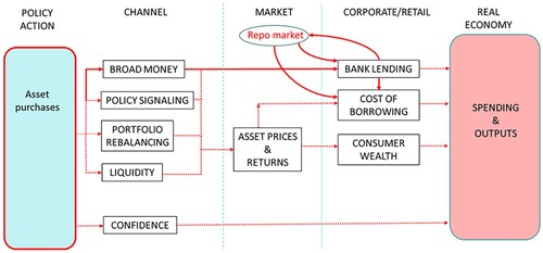
Our focus is on the broad money channel, where the additional liquidity banks receive leads to an increase in bank lending generally, and lending in the gilt repo market specifically. That is, QE operations lead to large increases in the amounts of reserves of certain banks. These banks may supply part of these additional reserves in the short-term funding markets, increasing liquidity and reducing spreads. As Figure 1 illustrates, this would reduce the cost of borrowing in the economy directly, by lowering the cost of borrowing for corporates in the repo market, and indirectly, by reducing the cost of funding for financial intermediaries, and hence the cost of credit they provide to the real economy. This paper contributes to the strand of the literature assessing the transmission of QE effects via the bank lending channel. For instance, Rodnyansky and Darmouni (2017) find evidence of the positive effects impact of QE on the lending behaviour of US banks, during the first and third waves of the Federal Reserves’ Large Scale Asset Purchases (LSAPs), but not during the second wave, which focused on government securities. Similar studies on the UK QE indicate very limited effects of QE on bank lending during earlier waves between 2009 and 2012 (Fatouh, Giansante, and Ongena 2021; Joyce and Spaltro 2014; and Giansante, Fatouh, and Ongena 2022), but stronger positive effects during later waves following the 2016 Brexit vote and Covid stress in 2020 (Fatouh, Markose, and Giansante 2021). Fatouh, Markose, and Giansante 2021 argue that these differences can be attributed to the relatively stronger bank capital positions during more recent waves and the lending support schemes introduced by the UK government during the Covid-19 pandemic.

Moreover, while assessing QE effects on bank balance sheets, Fatouh, Markose, and Giansante (2021) suggest that reserves injections increased recipient banks’ engagement in the repo market during the COVID stress period. QE purchases are generally initiated at times central banks deem as turbulent, during which repo markets, in particular the overnight market, tend to show signs of strain (Hüser, Lepore, and Veraart 2021). Hence, by improving the provision of liquidity, QE operations can help stabilise and improve the functioning of the repo market in stress. Additionally, banks’ incentives to do so are largely affected by capital requirements they are subject to, especially the leverage ratio capital requirements. The leverage ratio is a risk-agnostic requirement, under which no risk weights are assigned to exposures with different levels of risk. As such, it can affect low-risk activities (such as repo lending) disproportionally more (for example, Acosta-Smith, Grill, and Lang 2020).

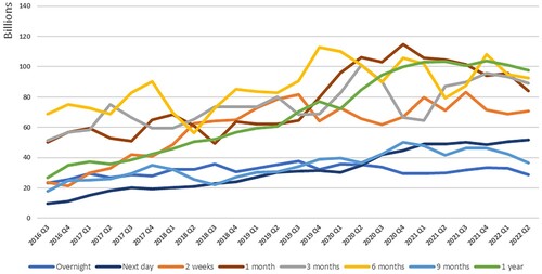
This paper aims to assess the impact of UK QE on liquidity and the cost of borrowing in the gilt repo market through the additional central bank reserves injected into the banking system in the two most recent QE waves following the Brexit vote (QE_Brexit) and during the Covid-19 stress (QE_Covid). It also considers the possible effects of the UK leverage ratio on the banks’ incentives to engage in repo transactions (see for example, Kotidis and van Horen 2018; and Gerba and Katsoulis 2021). We focus on the gilt repo market, the fourth largest repo market in the world, in terms of amounts outstanding (Committee on the Global Financial System 2017). Figure 2 shows the average daily volumes of reverse repo (lending) transactions in the market between 2016 Q3 and 2022 Q2.

Figure 2. Average daily amounts outstanding of reverse repo in the gilt repo market Source: Bank of England Database: https://www.bankofengland.co.uk/boeapps/database/default.asp. Series codes: YWQZM5L YWQZM5M YWQZM5O YWQZM5P YWQZM5Q YWQZM5R YWQZM5S YWQZM5T YWQZM6E.

We assess whether banks that received additional reserves through QE operations increased liquidity provision and reduced spreads in the gilt repo market. More specifically, our analysis aims to examine the impact of QE on spreads and amounts borrowed and lent in the gilt repo market, the pricing of individual transactions, and the effects of leverage ratio on amounts and pricing in that market. The analysis also seeks to assess whether the leverage ratio affected liquidity and spreads in the gilt repo market. To do so, we implement a difference-in-differences (DiD) setup, relying on a confidential Bank of England dataset, which identifies banks that received reserve injections through the asset purchase programme (APP). The setup follows Giansante, Fatouh, and Ongena (2022) by using a propensity score matching to avoid the QE treatment effect being contaminated by differences in bank characteristics between the treatment and control groups. The dataset combines three confidential data sources, including data on APP operations, gilt repo data from the Sterling Money Market Database (SMMD), and balance sheet data from regulatory returns.

Our results suggest that QE can improve liquidity provision in the gilt repo market, but the manner through which this is attained relies on the size of QE injection. While banks rely on the substantial liquidity of large QE injections (e.g. QE_Covid) to increase repo lending,¹ they tend to intermediate (i.e. borrow and lend) more when reserves injections are relatively smaller (e.g. QE_Brexit). QE can also reduce the cost of borrowing in the repo market, but this effect can disappear if demand in the market is quite strong, in the manner seen during the ‘dash for cash’ in March 2020. The period saw steep rises in demand for liquidity, especially by non-financial corporates concerned about their ability to withstand the shock caused by the pandemic, with many pre-emptively drawing-down existing credit lines to build cash reserves (Basel Committee on Banking Supervision 2021).²

Lastly, the results indicate that the leverage ratio supports the provision of liquidity in the repo market in stress, as it prompts banks to become less leveraged and hence enter stress with better balance sheet capacity. However, due to its risk insensitivity, the leverage ratio increases the amount of capital needed to support repo transactions relative to other activities. This effect reflects on the spreads of these transactions. We find evidence that banks subject to the ratio charged more on repo lending and paid less on repo borrowing.³

We contribute to the literature in several ways. Our analysis contributes to the literature assessing the repo market behaviour under stress. Earlier studies included assessments for repo markets in the US (Avalos, Ehlers, and Eren 2019; Copeland, Martin, and Walker 2014; Krishnamurthy, Nagel, and Orlov 2014; and Correa, Du, and Liao 2020), the Euro Area (Mancini, Ranaldo, and Wrampelmeyer 2016; and Boissel et al. 2017), and the UK (Hüser, Lepore, and Veraart 2021), as well as the effects of central bank intervention during COVID stress on that market (He, Nagel, and Song 2022). As mentioned earlier, we also contribute to the literature assessing QE transmission channels, specifically the impact on bank lending and bank balance sheets (for instance, Fatouh, Giansante, and Ongena 2021a; Fatouh, Markose, and Giansante 2021b; and Giansante, Fatouh, and Ongena 2022). Lastly, we add to the growing literature examining the effects of the post Great Financial Crisis (GFC) regulatory reforms (the leverage ratio in particular) on the liquidity and pricing in the repo market (for example, Bicu-Lieb, Chen, and Elliott 2020; Fatouh, Markose, and Giansante 2021; Kotidis and van Horen 2018; Noss and Patel 2019; and Gerba and Katsoulis 2021).

The remainder of the paper is structured as follows. Section 2 describes the data used; Section 3 explains the empirical design; Section 4 presents the results; Section 5 includes robustness checks; and Section 6 concludes.

2. Data

We use multiple confidential datasets held by the Bank. The first dataset covers QE operations by the Bank of England and includes information about banks that received reserve injections and the size of these injections. Following Giansante, Fatouh, and Ongena (2022), this dataset allows us to attain a perfect identification for our treatment group in a difference-in-differences (DiD) setup. Second, we use data on gilt repo transactions from the Sterling Money Market Database (SMMD). SMMD covers secured and unsecured lending and borrowing transactions carried out by the 33 most active dealers in the sterling money market, representing more than 90% of all transactions, on a daily basis. It contains transaction-level details on volumes, spreads, counterparties, and collateral types. Our dataset spans from January 2016 to April 2021, with about 4.11mn transactions, of which 1.97mn were lending (reverse repo) and the remainder were borrowing (repo) transactions. Lastly, we use internal regulatory data submitted (quarterly) by banks to collect data on bank-level controls. These returns include detailed information about banks’ assets composition, capitalisation, and riskiness. Table 1 provides an overview of our dataset. The Table provides variable definitions for both bank-level and transaction-level data alongside descriptive statistics.

Table 1. Descriptive statistics of the dataset.

Variable		Obs.	mean	St. dev	Min	P25	median	P75	Max
Trade-level
Amount	Log of amount borrowed or lent (cash leg of the trade)	4,109,107	16.91378	1.301885	12.27746	16.1159	17.07136	17.78374	22.1519
Spread* (%)	Spread over the reference rate index (to calculate interest rate at issuance)	4,109,107	−0.0169279	0.1354192	−3.1665	−0.0501	−0.008	0.03	182.542
maturity bucket	Maturity of the trade at issuance in years	4,109,107	0.0161702	0.0741871	0.0013699	0.0013699	0.0013699	0.0013699	1
Bank-level
totAssets	Log of total assets	352	25.16366	2.714524	13.91972	23.98957	25.92452	27.22304	28.22435
Rwa	Log of risk weighted assets	352	24.27514	3.021395	9.977574	23.64253	25.24683	25.99111	27.41535
Lem	Log of leverage ratio exposure measure	352	25.65179	2.632744	13.91972	25.10503	26.48531	27.35131	28.47689
cet1Cap	Log of core tier 1 capital	352	22.58127	2.359405	12.4285	22.01448	23.2494	24.106	25.36766
tier1Cap	Log of tier 1 capital	352	22.69106	2.389325	12.4285	22.01448	23.44739	24.21319	25.53545
trdAssets	Log of total trading assets	285	23.59532	3.308831	9.283219	22.72902	24.77246	25.3961	27.82987
securitiesAssets	Log of total securities holdings	349	22.83931	3.071773	9.92564	21.67911	23.60409	25.08148	27.05477
loansBanks	Log of total lending to banks	343	22.10879	3.101762	9.828926	20.0111	22.6904	24.53215	27.1546
totLoans	Log of total loans	346	23.83968	2.959396	11.9591	21.92683	24.96898	26.27623	27.4483
Npl	Non-performing loans/total loans		0.0367954	0.1163406	0	0.0030009	0.0139795	0.0298776	0.0929210
totLiabs	Log of total liabilities	351	25.06824	2.945941	8.994103	23.96959	25.87486	27.18127	28.17011
totDeposits	Log of total deposits	169	24.7924	3.320296	6.907755	24.0883	25.94362	26.96937	27.58602
Amount	Log of total amount lent/borrowed by a bank in a day per maturity bucket, LR nettability and collateral type	195,589	19.42061	1.752594	13.81551	18.30774	19.48539	20.74307	23.98591
Spread (%)	Weighted average spread on lending/borrowing by a bank in a day per maturity bucket, LR nettability and collateral type	195,589	0.0112572	0.1953133	−2.374435	−0.0414	0.003	0.0491144	53.5329

Source: Bank of England Sterling Money Market database, asset purchase facility operations database, and internal regulatory data.

*Spread: the difference between the rate charged and the relevant reference rates. Amounts are in logarithmic scale.

Out of the 33 broker-dealer banks in our sample, 22 received reserves injections via QE operations, and are hence designated as treated banks (QE banks). The remaining 11 are control banks (non-QE banks). Lastly, 11 banks are subject to leverage ratio requirements.⁴ Note that, as we will discuss in the empirical section, QE banks tend to be riskier than non-QE banks. In other words, non-QE banks show lower risk weight density. QE banks also have stronger capitalisation and hold repo portfolios with relatively shorter maturities. To alleviate these differences, we employ a propensity score matching using these dimensions as covariates as well as controlling for them in the DiD models.

3. Empirical design

To assess QE's effects on the pricing and amounts in the gilt repo market, we implement a DiD model that compares QE banks to banks that did not receive reserves injections (non-QE banks). Our baseline DiD model is: (1) $\begin{array}{r}{Y}_{i,t}={\beta }_i+{\omega }_j+{\delta }_1(\mathrm{Treate}{d}_i\mathit{Q}{\mathit{E}}_t)+{\delta }_2(\mathrm{Treate}{d}_i\mathit{Q}{\mathit{E}}_{t}L{R}_i)+{\gamma }_1\mathit{Q}{\mathit{E}}_t+\theta X_{i,t}+\varsigma (X_{i,t}\mathit{Q}{\mathit{E}}_t)+{\upsilon }_{i,t}\end{array}$(1) where $Y_{i,t}$: spread or log of lending amount; ${\beta }_i\mathrm{and}{\omega }_j$: bank and counterparty sector fixed effects; $\mathrm{Treate}{d}_i$: treatment dummy, set to 1 for QE banks and 0 otherwise; $\mathit{Q}{\mathit{E}}_t=[Q{E}_{\mathrm{Brexit},t},Q{E}_{\mathrm{Covid},t}]$: Brexit and Covid treatment time dummies, which are set to 0 before 4 August 2016 and 19 March 2020, respectively, and 1 afterwards; $L{R}_i$: leverage ratio dummy, set to 1 for banks subject to the leverage ratio framework and 0 otherwise; $\mathrm{Treate}{d}_i\mathit{Q}{\mathit{E}}_t$: interaction term of treatment and QE episode; $\mathrm{Treate}{d}_i\mathit{Q}{\mathit{E}}_{t}L{R}_i$: interaction term of treatment, QE episode and leverage ratio requirements; $X_{i,t}$: a matrix of controls, including bank-level and transaction-level controls. As shown in Table 1, bank-level controls include balance sheet assets and liabilities, capitalisation metrics, and risk measures (risk-weighted assets and non-performing loans). Transaction-level controls include maturity, collateral type, central clearing dummy (set to 1 for transactions cleared with a central counterparty, CCP, and 0 otherwise), and leverage ratio nettability dummy (set to 1 for transactions eligible for netting under the leverage ratio rules and 0 for ineligible transactions)⁵; $X_{i,t}\ast \mathit{Q}{\mathit{E}}_t$: interaction terms to account for possible heterogeneous responses by banks. We apply Equation (1) at both the bank-level, where we assess effects on daily total amounts and weighted average spreads charged and paid by banks, and the transaction-level, where we assess the impact on spreads of individual transactions. In both analyses, we categorise transactions into three maturity buckets, overnight (we refer to as short-term), two weeks to one month (we refer to as medium-term), and three months to one year (we refer to as long-term).⁶

The selection of QE banks (i.e. selection into the treatment group) is most likely not random. It would probably reflect specific bank characteristics, such as bank size and the structure of assets and liabilities. Hence, our analysis and results could be influenced by selection bias. To mitigate this, and create comparable treatment and control groups, we use a propensity score matching approach. We implement the matching in three stages. First, we check whether selection to treatment is correlated with certain bank and repo portfolio characteristics. To do so, we regress the treatment status (dummy) before the treatment (i.e. QE waves) on a set of bank-level variables, reflecting business model, risk, and capitalisation, as well as repo portfolio-level variables, reflecting size and maturity. We do that for lending (reverse repo) and borrowing (repo) separately, and for the total lending and borrowing portfolios as well as sub-portfolios/maturity buckets (short-term, medium-term, and long-term). We also do this assessment before the Brexit and Covid waves separately, unlike Giansante, Fatouh, and Ongena (2022), who do the assessment just before the first two waves. This is because bank-level data coverage is somewhat less complete before the QE_Brexit, which affects our ability to do comprehensive matching. In the next step, we use characteristics correlated with the treatment status to match each bank in the treatment group with those in the control group that are most similar based on these characteristics. Lastly, we rerun the regressions we did in the first step (treatment on characteristics) using the matched sample, to verify whether the matching has reduced differences between the treatment and control groups. Worth noting that, following Fatouh, Giansante, and Ongena (2024), in one of our robustness tests we implement an alternative matching approach with our DiD models using entropy balancing suggested by Hainmueller and Xu (2013).

4. Analysis and results

4.1. Propensity score matching

As mentioned above, we regress treatment status on a set of bank-level and portfolio-level variables, separately for lending and borrowing portfolios, as well as for total portfolios and sub-portfolios (short-term, medium-term, and long-term). For the total portfolios, the portfolio-level variables include the log of the total amount (lent/borrowed) and the weighted average maturity of all (lending/borrowing) transactions. Meanwhile, the sub-portfolios, include the log of the amounts in the sub-portfolios and the percentages of the amounts in the sub-portfolios out of the amounts in the total portfolios. The bank-level variables include size (total assets), risk-weighted assets (RWAs), and capitalisation (core equity tier 1, CET1, ratio). The results of the regressions are presented under models (1) in Tables 2 and 3. As the two tables show, on average, treated banks are smaller, and have higher risk weight density (i.e. higher RWAs), stronger capitalisation, and repo portfolios with relatively shorter maturities. We then match each bank in the treatment group with the most similar banks in terms of these characteristics in the control group. We use a 1:2 matching ratio in our baseline to better balance the two groups. That is, each treated bank is matched with the most similar two banks in the control group based on the abovementioned characteristics.⁷ After the matching, we re-run the same (pre-matching) regressions, but using the matched sample, and results are shown in models (2) in Tabled 2 and 3. Comparing the results of models (1) and models (2) regressions indicates that the matching generally reduces differences between the treatment and control groups,⁸ and hence we can proceed to the baseline regressions (Equation (1)) at both the bank-level and the transaction-level. As mentioned above, we also use entropy balancing as an alternative matching technique in one of our robustness checks in Section 5.

Table 2. Propensity score matching (pre Brexit QE).

	Lending (reverse repo)								Borrowing (repo)
	All maturities		Overnight		2 weeks to 1 month		3 months or more		All maturities		Overnight		2 weeks to 1 month		3 months or more
	(1)	(2)	(1)	(2)	(1)	(2)	(1)	(2)	(1)	(2)	(1)	(2)	(1)	(2)	(1)	(2)
VARIABLES	treat	treat	treat	treat	treat	treat	treat	treat	treat	treat	treat	treat	treat	treat	treat	treat
Total amount	−0.495	−0.057	−14.443	−2.408	−1.343	−1.202	0.050	−0.396	0.182	0.080	0.255	0.062	−0.257	−0.491*	−0.463	−0.688
	(0.303)	(0.200)	(19.972)	(1.973)	(1.089)	(1.657)	(0.190)	(0.411)	(0.179)	(0.180)	(0.174)	(0.169)	(0.231)	(0.286)	(0.368)	(0.488)
w. avg. maturity	−22.642	2.548							−13.379***	−7.885
	(15.940)	(14.380)							(4.725)	(29.879)
pct. Of total portfolio			157.854	22.484	−6.141*	−2.626	−5.263	−0.261			0.258	0.548	3.468	4.968*	13.907	21.223
			(220.803)	(15.317)	(3.236)	(4.350)	(8.013)	(10.664)			(0.169)	(0.337)	(2.431)	(2.661)	(12.193)	(15.022)
Total assets	−0.806***	−0.724*	−21.692	−3.463	−2.014*	−1.920	−0.662***	−0.500	−0.125	−0.153	0.059	−0.080	0.365	0.497*	0.220	0.386
	(0.302)	(0.439)	(30.499)	(1.942)	(1.059)	(1.818)	(0.218)	(0.385)	(0.121)	(0.202)	(0.123)	(0.161)	(0.285)	(0.271)	(0.217)	(0.296)
RWAs	1.365**	2.440**	37.062	6.695	4.322	4.078	1.107**	2.144*
	(0.642)	(1.133)	(51.809)	(3.335)	(2.726)	(3.930)	(0.505)	(1.199)
CET1 ratio	13.628	65.345	77.036	61.118	49.267	48.434	9.183	62.038
	(11.477)	(40.846)	(76.983)	(41.781)	(47.046)	(62.553)	(6.782)	(45.579)
Constant	−2.037	−30.212*	−141.664	−44.790**	−30.965	−32.095	−13.781	−40.927*	−0.726	1.258	−7.590	−0.649	−1.364	0.107	6.425	6.727
	(15.448)	(18.366)	(194.956)	(18.494)	(27.054)	(28.914)	(11.227)	(23.686)	(5.510)	(8.353)	(5.350)	(6.733)	(8.981)	(6.101)	(9.138)	(9.883)
Matching	-pre	-post	-pre	-post	-pre	-post	-pre	-post	-pre	-post	-pre	-post	-pre	-post	-pre	-post
$\mathrm{Adj}{R}^2$	0.498	0.494	0.669	0.598	0.586	0.442	0.430	0.340	0.355	0.126	0.338	0.244	0.242	0.364	0.291	0.432
p-value	0.000	0.101	0.688	0.151	0.002	0.333	0.007	0.489	0.027	0.619	0.046	0.115	0.368	0.233	0.496	0.473
N	17	14	17	13	16	12	16	13	13	12	13	13	12	12	11	11

Probit regressing the treatment on lending/borrowing (reverse repo/repo) portfolio characteristics and bank characteristics. The dependent variable is QE treatment status treat for QE banks. Model (1) reports the pre-matching results while model (2) reports the post matching results with matching ratio 1:2. Coefficients and standard errors are reported for each variable. Standard errors are robust and reported in brackets, *p < 0.10, **p < 0.05, ***p < 0.01.

Table 3. Propensity score matching (pre Covid QE).

	Lending (reverse repo)								Borrowing (repo)
	All maturities		Overnight		2 weeks to 1 month		3 months or more		All maturities		Overnight		2 weeks to 1 month		3 months or more
	(1)	(2)	(1)	(2)	(1)	(2)	(1)	(2)	(1)	(2)	(1)	(2)	(1)	(2)	(1)	(2)
VARIABLES	treat	treat	treat	treat	treat	treat	treat	treat	treat	treat	treat	treat	treat	treat	treat	treat
Total amount	0.050	−0.189	0.059	−0.212	0.001	−0.169	−0.074	0.103	0.080	−1.352***	0.117	−0.029	−0.005	−0.119	−0.024	−0.101
	(0.171)	(0.172)	(0.164)	(0.176)	(0.215)	(0.272)	(0.218)	(0.236)	(0.127)	(0.422)	(0.107)	(0.132)	(0.155)	(0.177)	(0.128)	(0.146)
w. avg. maturity	−23.157**	−9.880							−5.720	413.900
	(11.559)	(16.021)							(8.014)	(172.524)
pct. Of total portfolio			4.647**	1.191	−6.003	1.183	−10.392*	−9.771*			−0.041	−0.009	−1.487	0.334	−4.041	6.796
			(2.289)	(2.786)	(3.834)	(3.274)	(5.786)	(5.341)			(0.074)	(0.063)	(2.681)	(2.337)	(7.919)	(9.241)
Total assets	−3.026***	−2.783*	−3.259***	−2.594*	−3.187**	−2.210**	−2.699***	−1.941**	−2.199***	−1.183	−2.160***	−2.516***	−2.072***	−2.295***	−2.026***	−2.335***
	(0.842)	(1.457)	(1.047)	(1.400)	(1.322)	(0.912)	(0.793)	(0.835)	(0.814)	(0.893)	(0.733)	(0.956)	(0.676)	(0.695)	(0.686)	(0.860)
RWAs	3.370***	2.683*	3.595***	2.487*	3.491**	2.119**	3.028***	1.813**	2.319***	2.244*	2.392***	2.427**	2.343***	2.360***	2.269***	2.339**
	(0.924)	(1.405)	(1.135)	(1.367)	(1.439)	(0.947)	(0.914)	(0.802)	(0.826)	(1.254)	(0.775)	(0.986)	(0.723)	(0.742)	(0.732)	(0.926)
CET1 ratio	10.964	20.929	13.785	22.331	14.644	20.694	10.865	32.142	4.067***	63.367**	4.671***	5.506	6.681	9.260	5.264	5.799
	(7.097)	(18.458)	(9.761)	(18.338)	(11.567)	(16.546)	(7.196)	(24.323)	(1.360)	(25.104)	(1.310)	(8.314)	(6.455)	(6.201)	(5.743)	(5.821)
Constant	−7.754	6.906	−12.456*	6.033	−5.640	4.818	−4.737	−2.157	−2.998	−0.427	−6.937	4.443	−4.820	1.729	−3.630	3.189
	(6.750)	(13.684)	(7.350)	(12.329)	(6.038)	(13.952)	(4.546)	(5.392)	(8.794)	(11.803)	(4.231)	(9.482)	(5.757)	(5.990)	(5.424)	(6.477)
Matching	-pre	-post	-pre	-post	-pre	-post	-pre	-post	-pre	-post	-pre	-post	-pre	-post	-pre	-post
$\mathrm{Adj}{R}^2$	0.550	0.483	0.563	0.475	0.545	0.487	0.530	0.439	0.465	0.675	0.465	0.489	0.445	0.446	0.434	0.468
p-value	0.008	0.257	0.031	0.383	0.109	0.152	0.019	0.206	0.003	0.022	0.008	0.149	0.033	0.026	0.032	0.032
N	33	28	33	28	31	26	31	26	30	26	30	29	29	29	28	28

Probit regressing the treatment on lending/borrowing (reverse repo/repo) portfolio characteristics and bank characteristics. The dependent variable is QE treatment status treat for QE banks. Model (1) reports the pre-matching results while model (2) reports the post matching results with matching ratio 1:2. Coefficients and standard errors are reported for each variable. Standard errors are robust and reported in brackets, *p < 0.10, **p < 0.05, ***p < 0.01.

4.2. Bank-level analysis

We start our analysis by running Equation (1) at the bank-level, where we assess the treatment effects on the daily amounts lent and borrowed and the spreads charged and paid by QE banks, compared to the control group. Amounts are the sums of amounts lent and borrowed in the aggregate and sub-portfolios, as indicated earlier. Spreads are weighted averages of spreads on individual transactions within each maturity bucket on each date, using transaction amounts as weights. Table 4 presents the DiD results for bank-level models. The results of the equivalent DiD regressions based on entropy balancing are shown in Table A1 and are largely consistent with the baseline results displayed in Table 4.⁹

Table 4. QE treatment effect – bank-level.

Panel (a): reverse repo (lending) amounts and pricing
	Amounts				Spreads
Variables	All 1(a)	Overnight 1(b)	2 weeks to 1 month 1(c)	3 months or more 1(d)	All 1(a)	Overnight 1(b)	2 weeks to 1 month 1(c)	3 months or more 1(d)
$\mathit{Treated}\times \mathit{Q}{\mathit{E}}_{\mathit{Brexit},\mathit{t}}$	−0.149	1.852**	−0.149	−0.528***	−0.0879**	−0.133***	−0.0661***	−0.0310***
	(0.519)	(0.915)	(0.0139)	(0.162)	(0.0428)	(0.00755)	(0.0140)	(0.00723)
$\mathrm{Treated}\times Q{E}_{\mathrm{Brexit},t}\times L{R}_t$	0.253	0.547	−0.0648	0.195	−0.0662***	−0.0927***	−0.0242***	0.0265***
	(1.0797)	(1.115)	(0.129)	(0.253)	(0.0162)	(0.00895)	(0.00261)	(0.00590)
Obs.	33,679	16,428	10,956	5,468	33,679	16,428	10,956	5,007
R-squared	0.117	0.111	0.124	0.111	0.021	0.198	0.012	0.094
$\mathrm{Treated}\times Q{E}_{\mathrm{Covid},t}$	0.336***	0.383***	−0.297	0.376*	0.0120	0.0000384	−0.0210	0.00780
	(0.157)	(0.0817)	(0.256)	(0.203)	(0.0145)	(0.0222)	(0.0237)	(0.0204)
.$\mathrm{Treated}\times Q{E}_{\mathrm{Covid},t}\times L{R}_t$	0.684***	0.975**	−0.0493	0.699***	0.000850	−0.00322	−0.00616	0.0121
	(0.254)	(0.385)	(0.222)	(0.159)	(0.0129)	(0.0246)	(0.0182)	(0.0150)
Obs.	8,978	4,382	2,881	1,654	8,978	4,382	2,881	1,654
R-squared	0.269	0.576	0.260	0.348	0.178	0.663	0.232	0.141
QE	Yes	Yes	Yes	Yes	Yes	Yes	Yes	Yes
LR	Yes	Yes	Yes	Yes	Yes	Yes	Yes	Yes
Ctrls	Yes	Yes	Yes	Yes	Yes	Yes	Yes	Yes
Ctrls * QE	Yes	Yes	Yes	Yes	Yes	Yes	Yes	Yes
Bank FEs	Yes	Yes	Yes	Yes	Yes	Yes	Yes	Yes
Coefficient estimates of amounts and spreads on reverse repo (lending) on daily basis (Jan 2016 to Apr 2021). $\mathrm{Treate}{d}_i$ equals to 1 for QE banks and 0 for non-QE banks. Controls include bank-level controls (e.g. total assets, RWAs) and portfolio-level controls (e.g. maturity bucket, collateral type). Robust standard errors reported between parentheses, *p < 0.10, **p < 0.05, ***p < 0.01.
$\mathrm{Treated}\times Q{E}_{\mathrm{Brexit},t}$	0.428***	0.900***	−1.538***	−0.0725	0.0000424	0.00899	−0.0709*	0.0532
	(0.143)	(0.162)	(0.209)	(0.550)	(0.0263)	(0.00760)	(0.0395)	(0.0597)
$\mathrm{Treated}\times Q{E}_{\mathrm{Brexit},t}\times L{R}_t$	−0.170*	−0.158	0.659***	0.808***	−0.0753***	−0.0578***	−0.131***	−0.0781***
	(0.0999)	(0.126)	(0.125)	(0.171)	(0.0222)	(0.00564)	(0.0469)	(0.00698)
Obs.	13,847	24,952	16,623	8,748	49,246	24,952	16,623	8,748
R-squared	0.295	0.233	0.141	0.101	0.017	0.065	0.013	0.068
$\mathrm{Treated}\times Q{E}_{\mathrm{Covid},t}$	0.122	−0.0378	0.329	0.134	0.0373***	0.0409***	0.0186	−0.0109
	(0.117)	(0.172)	(0.225)	(0.220)	(0.00852)	(0.0130)	(0.0130)	(0.0130)
.$\mathrm{Treated}\times Q{E}_{\mathrm{Covid},t}\times L{R}_t$	0.128	0.0914	0.0520	0.125	−0.00200	−0.0422***	0.0116	0.0320***
	(0.100)	(0.174)	(0.186)	(0.212)	(0.00521)	(0.00851)	(0.00746)	(0.00983)
Obs.	19,692	10,126	6,520	3,877	19,692	10,126	6,520	3,877
R-squared	0.380	0.403	0.382	0.490	0.600	0.662	0.609	0.706
QE	Yes	Yes	Yes	Yes	Yes	Yes	Yes	Yes
LR	Yes	Yes	Yes	Yes	Yes	Yes	Yes	Yes
Ctrls	Yes	Yes	Yes	Yes	Yes	Yes	Yes	Yes
Ctrls * QE	Yes	Yes	Yes	Yes	Yes	Yes	Yes	Yes
Bank Fes	Yes	Yes	Yes	Yes	Yes	Yes	Yes	Yes

Coefficient estimates of amounts and spreads on repo (borrowing) on daily basis (Jan 2016 to Apr 2021). $\mathrm{Treate}{d}_i$ equals to 1 for QE banks and 0 for non-QE banks. Controls include bank-level controls (e.g. total assets, RWAs) and portfolio-level controls (e.g. maturity bucket, collateral type). Robust standard errors reported between parentheses, * p < 0.10 ** p < 0.05 *** p < 0.01.

4.2.1. QE effects

As the top part of Panel (a) shows, relative to the control group, QE banks did not increase their total lending post QE_Brexit. They, however, restructured reverse repo portfolios towards significantly less long-term lending and significantly more short-term lending. Meanwhile, post QE_Covid, QE banks total repo lending was 33.6% higher than that of non-QE banks. The effects are clearer for short-term lending, which was 38.3% higher for QE banks. A weaker and less significant increase is seen for long-term lending, and no statistically significant effects can be documented for medium-term lending.

Contrary to QE_Brexit, the ample size of reserves injections through the large QE purchases during QE_Covid allowed QE banks to satisfy the very high demand for short-term liquidity during the March 2020 dash-for-cash without rationing longer-term lending. During QE_Brexit, the increased lending by QE banks was supported by rationing longer-term lending, as well as increased borrowing. As Panel (b) suggests, total and especially short-term borrowing of QE banks increased by 42.8% and 90% (respectively) post QE_Brexit, but shows no statistically significant change post QE_Covid, relative to the control group. Thus, QE operations helped improve the provision of liquidity in the gilt repo market by injecting additional reserves and incentivising banks that received those reserves to increase the level of intermediation in the market (borrowing and lending more). The latter is more apparent in the QE_Brexit and less so in QE_Covid due to the larger reserves injections during QE_Covid.

In terms of pricing, spreads charged by QE banks were about 8.8bps lower than those of non-QE banks post QE_Brexit. However, the spreads of the two groups of banks show no statistically significant differences after QE_Covid, probably due to the very strong demand at the time when that wave was introduced.

In summary, we find evidence that QE improves liquidity provision in the gilt repo market, specifically in the overnight segment of the market. However, the size of QE injection dictates how this increased provision is attained. When injections are sufficiently large (e.g. QE_Covid), the sizeable liquidity provided by QE purchases support the increased liquidity provision. Meanwhile, the higher provision following smaller injections (e.g. QE_Brexit) would be funded by a mix of rationing of longer-term lending and increased repo borrowing. In other words, smaller QE injection can increase intermediation in the short-term gilt repo market. The additional cheaper liquidity received via QE operations can reduce the cost of funding in the gilt repo market, but demand factors can reduce this effect or wipe it out entirely.

4.2.2. Leverage ratio effects

The total lending of QE banks subject to the leverage ratio was 68.4% higher during QE_Covid, but showed no statistically significant difference during QE_Brexit, compared to the control group. This indicates that the leverage ratio did not have a negative impact on bank lending in the gilt repo market. On the contrary, by comparing to the treatment effect of all QE banks during QE_Covid, the leverage ratio had a net positive effect on that lending.¹⁰ Nevertheless, the difference in effects between the two waves is likely arising from the chronical sequence of the leverage ratio implementation. The ratio was introduced in 2016 as a risk-agnostic measure into a regulatory framework characterised by risk-weighted capital requirements. Hence, at its introduction, the leverage ratio would have had some effects on banks’ incentives to engage in low-risk activities (with low capital requirements), such as repo lending, as it leads to an increase in the capital base required to support these activities compared to riskier activities. This explains why QE banks subject to the leverage ratio lending did not increase lending and charged higher spreads during QE_Brexit, which came only 8 months after the leverage ratio introduction. In terms of pricing, QE banks subject to leverage ratio charged relatively more on repo lending compared to other QE banks, but still less than the control group.¹¹ The clearer effects during QE_Brexit are likely due to the lower liquidity injected into the system via QE, and the possible effects of the recent introduction of the leverage ratio on low-risk activities. Moreover, QE banks subject to the leverage ratio paid less on repo borrowing compared to the control group as well as other QE banks. This is because repo borrowing transactions attract capital charges in the leverage ratio, making this source of funding relatively more costly (economically) for banks subject to the ratio, and reducing the spreads they are willing to pay to attain it.

To sum up, our results suggest that the leverage ratio not only has no negative effects on the provision of liquidity in the gilt repo market, but also can have positive effects on stress. Yet, the ratio increases the economic cost of repo lending for banks subject to it, increasing the spreads they charge on this lending. Our results are in line with those of Gerba and Katsoulis (2021). They, however, contrast with earlier studies that indicate the negative effects of the leverage ratio on the provision of low-risk activities (for instance, Kotidis and van Horen 2018; and Acosta-Smith, Grill, and Lang 2020). The two views can be reconciled. Earlier studies mostly cover the early stages after the introduction of the leverage ratio, when banks were still adjusting to the changes in the regulatory regime that would disproportionally affect low-risk activities, as discussed above. However, over time, after banks had adjusted to the new regulatory regime, leverage ratio effects would appear in the pricing of low-risk activities rather than their amounts. In fact, the leverage ratio can have ‘positive’ effects on the provision of low-risk activities in stress, as banks are subject to it to enter the stress with stronger capital positions. This likely explains the larger increase in lending by QE banks subject to the leverage ratio compared to both the control group and other QE banks not subject to the ratio.

4.3. Transaction-level analysis

In this section, we run the model in Equation (1) at the transaction-level, to assess whether the trends we document for spreads at the bank-level flow into the pricing of individual trades. Specifically, we assess whether the spreads charged on individual repo transactions by QE banks changed relative to similar transactions offered by the control group post QE episodes. We do that for each of the sub-portfolios (short-term, medium-term, and long-term) separately. Regression results are presented in models (a) of Tables 5 and 6.

Table 5. QE treatment effect on spreads and amounts of reverse repos – transaction-level.

Panel (a): Spreads
	Overnight			2 weeks to 1 month			3 months or more
Variables	1(a)	1(b)	1(c)	2(a)	2(b)	2(c)	3(a)	3(b)	3(c)
.$\mathrm{Treated}\times Q{E}_{\mathrm{Brexit},t}$	−0.0989***	−0.0868***	−0.0868***	−0.828	−1.375	−1.375	−0.500	−0.0554	−0.0554
	(0.0215)	(0.0213)	(0.0213)	(0.605)	(0.982)	(0.982)	(0.546)	(0.251)	(0.251)
$\mathrm{Treated}\times Q{E}_{\mathrm{Brexit},t}\times L{R}_t$	−0.0399***	−0.0281***	−0.0281***	0.880	1.190	1.190	0.0456	0.0526	0.0526
	(0.00170)	(0.00165)	(0.00165)	(0.772)	(1.896)	(1.896)	(0.0735)	(0.205)	(0.205)
.$\mathrm{Transactionamount}$	0.00132***	0.00169***	0.00169***	−0.00547***	−0.00179	−0.00179	−0.00894***	−0.00274***	−0.00274***
	(0.0000905)	(0.0000795)	(0.0000795)	(0.000216)	(0.00131)	(0.00131)	(0.00191)	(0.000497)	(0.000497)
Obs.	567,711	567,711	567,711	221,523	221,523	221,523	43,591	752	752
R-squared	0.079	0.147	0.147	0.113	0.169	0.169	0.241	0.296	0.296
.$\mathrm{Treated}\times Q{E}_{\mathrm{Covid},t}$	0.00334	0.00426	0.00426	−0.00216	0.00689	0.00689	−0.0714	−0.204***	−0.204***
	(0.00511)	(0.00506)	(0.00506)	(0.00790)	(0.00665)	(0.00665)	(0.0596)	(0.0596)	(0.0596)
.$\mathrm{Treated}\times Q{E}_{\mathrm{Covid},t}\times L{R}_t$	−0.0316***	−0.0328***	−0.0328***	−0.0157***	−0.00216	−0.00216	−0.147***	−0.149***	−0.149***
	(0.00566)	(0.00558)	(0.00558)	(0.00436)	(0.00410)	(0.00410)	(0.0443)	(0.0391)	(0.0391)
.$\mathrm{Transaction}\mathrm{amount}$	0.00223***	0.00225***	0.00225***	−0.00527***	0.00132*	0.00132*	−0.0173***	−0.00555	−0.00555
	(0.000736)	(0.000738)	(0.000738)	(0.000237)	(0.000759)	(0.000759)	(0.00584)	(0.00611)	(0.00611)
Obs.	43,591	43,591	43,591	221,523	221,523	221,523	43,591	752	752
R-squared	0.192	0.194	0.194	0.006	0.013	0.013	0.192	0.254	0.254
QE	Yes	Yes	Yes	Yes	Yes	Yes	Yes	Yes	Yes
LR	Yes	Yes	Yes	Yes	Yes	Yes	Yes	Yes	Yes
Ctrls	Yes	Yes	Yes	Yes	Yes	Yes	Yes	Yes	Yes
Ctrls * QE	Yes	Yes	Yes	Yes	Yes	Yes	Yes	Yes	Yes
Bank Fes	Yes	Yes	Yes	Yes	Yes	Yes	Yes	Yes	Yes
CP sec. Fes	No	Yes	Yes	No	Yes	Yes	No	Yes	Yes
LR nettability	No	Yes	No	No	Yes	No	No	Yes	No
Coefficient estimates of spreads on reverse repo transactions on daily basis (Jan 2016 to Apr 2021). Model specifications: (a) bank fixed-effect only; (b) bank, counterparty sector and LR nettability fixed-effects; and (c) bank and counterparty sector fixed-effects and LR nettability as a control. Treatment status$\mathrm{Treate}{d}_i$ equals to 1 for QE-banks and 0 for non-QE-banks. Controls include collateral type and central clearing status. Robust standard errors reported between parentheses, *p < 0.10, **p < 0.05, ***p < 0.01.
.$\mathrm{Treated}\times Q{E}_{\mathrm{Brexit},t}$	−0.587	−1.849***	−1.849***	−7.777**	−3.308	−3.308	0.386	0.392	0.3858684
	(0.466)	(0.461)	(0.461)	(3.500)	(4.791)	(4.791)	(0.751)	(0.700)	(0.708254)
.$\mathrm{Treated}\times Q{E}_{\mathrm{Brexit},t}\times L{R}_t$	−0.639***	−0.927***	−0.927***	−0.00913	0.294	0.294	1.434	−1.012	−0.9687634
	(0.0656)	(0.0645)	(0.0645)	(0.362)	(0.350)	(0.350)	(1.351)	(1.293)	(1.321237)
Obs.	567,711	567,711	567,711	57,536	57,536	57,536	34,168	34,168	34,168
R-squared	0.069	0.118	0.118	0.076	0.205	0.205	0.043	0.141	0.141
.$\mathrm{Treated}\times Q{E}_{\mathrm{Covid},t}$	0.303***	0.305***	0.305***	1.223***	1.074***	1.074***	0.109	0.127	0.127
	(0.0565)	(0.0564)	(0.0564)	(0.0941)	(0.0918)	(0.0918)	(0.807)	(0.602)	(0.602)
.$\mathrm{Treated}\times Q{E}_{\mathrm{Covid},t}\times L{R}_t$	0.0674	0.0566	0.0566	−0.243***	−0.295***	−0.295***	0.109	0.203	0.203
	(0.0614)	(0.0614)	(0.0614)	(0.0378)	(0.0346)	(0.0346)	(0.455)	(0.360)	(0.360)
Obs.	43,591	43,591	43,591	221,523	221,523	221,523	752	752	752
R-squared	0.143	0.145	0.145	0.093	0.247	0.247	0.276	0.432	0.432
QE	Yes	Yes	Yes	Yes	Yes	Yes	Yes	Yes	Yes
LR	Yes	Yes	Yes	Yes	Yes	Yes	Yes	Yes	Yes
Ctrls	Yes	Yes	Yes	Yes	Yes	Yes	Yes	Yes	Yes
Ctrls * QE	Yes	Yes	Yes	Yes	Yes	Yes	Yes	Yes	Yes
Bank FEs	Yes	Yes	Yes	Yes	Yes	Yes	Yes	Yes	Yes
CP sec. FEs	No	Yes	Yes	No	Yes	Yes	No	Yes	Yes
LR nettability	No	Yes	No	No	Yes	No	No	Yes	No

Coefficient estimates of amounts of reverse repo transactions on daily basis (Jan 2016 to Apr 2021). Model specifications: (a) bank fixed-effect only; (b) bank, counterparty sector and LR nettability fixed-effects; and (c) bank and counterparty sector fixed-effects and LR nettability as a control. Treatment status$\mathrm{Treate}{d}_i$ equals to 1 for QE-banks and 0 for non-QE-banks. Controls include collateral type and central clearing status. Robust standard errors reported between parentheses, *p < 0.10, **p < 0.05, ***p < 0.01.

Table 6. QE treatment effect on spreads and amounts of repos (borrowing) – transaction-level.

Panel (a): Spreads
	Overnight			2 weeks to 1 month			3 months or more
Variables	1(a)	1(b)	1(c)	2(a)	2(b)	2(c)	3(a)	3(b)	3(c)
.$\mathrm{Treated}\times Q{E}_{\mathrm{Brexit},t}$	0.0143***	0.0156***	0.0156***	−0.0751***	−0.0732***	−0.0732***	−0.150***	−0.146***	−0.146***
	(0.00242)	(0.00245)	(0.00245)	(0.0186)	(0.0184)	(0.0184)	(0.0571)	(0.0435)	(0.0435)
$\mathrm{Treated}\times Q{E}_{\mathrm{Brexit},t}\times L{R}_t$	−0.0338***	−0.0385***	−0.0385***	−0.0920***	−0.0829***	−0.0829***	−0.120***	−0.0715***	−0.0715***
	(0.00144)	(0.00138)	(0.00138)	(0.00331)	(0.00328)	(0.00328)	(0.0189)	(0.0161)	(0.0161)
.$\mathrm{Transactionamount}$	0.00181***	0.00224***	0.00224***	−0.000891***	−0.00581***	−0.00581***	0.0108***	−0.0000914	−0.0000914
	(0.0000971)	(0.0000999)	(0.0000999)	(0.000241)	(0.000255)	(0.000255)	(0.000826)	(0.000835)	(0.000835)
Obs.	1,174,064	1,174,064	1,174,064	168,563	168,563	168,563	11,897	11,897	11,897
R-squared	0.059	0.068	0.068	0.053	0.110	0.110	0.157	0.298	0.298
..$\mathrm{Treated}\times Q{E}_{\mathrm{Covid},t}$	−0.258***	0.00443	0.00443	−0.117***	−0.0220	−0.0220	−0.474***	0.0518***	0.0518***
	(0.0190)	(0.00273)	(0.00273)	(0.0421)	(0.0157)	(0.0157)	(0.0490)	(0.0112)	(0.0112)
.$\mathrm{Treated}\times Q{E}_{\mathrm{Covid},t}\times L{R}_t$	0.00672**	−0.00746***	−0.00746***	−0.0198	−0.0134*	−0.0134*	0.0496***	−0.0369***	−0.0369***
	(0.00275)	(0.00197)	(0.00197)	(0.0155)	(0.00736)	(0.00736)	(0.0120)	(0.00783)	(0.00783)
.$\mathrm{Transactionamount}$	0.00506***	0.00448***	0.00448***	0.00161***	−0.000531	−0.000531	0.0113***	0.000468	0.000468
	(0.000198)	(0.000207)	(0.000207)	(0.000518)	(0.000618)	(0.000618)	(0.000666)	(0.000716)	(0.000716)
Obs.	130,763	130,763	130,763	14,332	14,332	14,332	19,337	19,337	19,337
R-squared	0.153	0.167	0.167	0.198	0.219	0.219	0.164	0.273	0.273
QE	Yes	Yes	Yes	Yes	Yes	Yes	Yes	Yes	Yes
LR	Yes	Yes	Yes	Yes	Yes	Yes	Yes	Yes	Yes
Ctrls	Yes	Yes	Yes	Yes	Yes	Yes	Yes	Yes	Yes
Ctrls * QE	Yes	Yes	Yes	Yes	Yes	Yes	Yes	Yes	Yes
Bank FEs	Yes	Yes	Yes	Yes	Yes	Yes	Yes	Yes	Yes
CP sec. FEs	No	Yes	Yes	No	Yes	Yes	No	Yes	Yes
LR nettability	No	Yes	No	No	Yes	No	No	Yes	No
Coefficient estimates of spreads on repo transactions on daily basis (Jan 2016 to Apr 2021). Model specifications: (a) bank fixed-effect only; (b) bank, counterparty sector and LR nettability fixed-effects; and (c) bank and counterparty sector fixed-effects and LR nettability as a control. Treatment status$\mathrm{Treate}{d}_i$ equals to 1 for QE-banks and 0 for non-QE-banks. Controls include collateral type and central clearing status. Robust standard errors reported between parentheses, *p < 0.10, **p < 0.05, ***p < 0.01.
.$\mathrm{Treated}\times Q{E}_{\mathrm{Brexit},t}$	0.0161	0.112***	0.112***	−0.506**	−0.344*	−0.344*	1.974***	1.225***	1.225***
	(0.0318)	(0.0316)	(0.0316)	(0.221)	(0.199)	(0.199)	(0.350)	(0.360)	(0.360)
.$\mathrm{Treated}\times Q{E}_{\mathrm{Brexit},t}\times L{R}_t$	0.0588***	0.121***	0.121***	0.0316	−0.0245	−0.0245	−0.743***	−0.538**	−0.538**
	(0.0189)	(0.0180)	(0.0180)	(0.0540)	(0.0489)	(0.0489)	(0.276)	(0.223)	(0.223)
Obs.	1,174,064	1,174,064	1,174,064	168,563	168,563	168,563	11,897	11,897	11,897
R-squared	0.110	0.149	0.149	0.073	0.205	0.205	0.162	0.345	0.345
.$\mathrm{Treated}\times Q{E}_{\mathrm{Covid},t}$	0.00474	−0.136***	−0.136***	0.719***	0.293***	0.293***	0.683***	0.341**	0.341**
	(0.0346)	(0.0352)	(0.0352)	(0.105)	(0.0955)	(0.0955)	(0.171)	(0.138)	(0.138)
.$\mathrm{Treated}\times Q{E}_{\mathrm{Covid},t}\times L{R}_t$	0.416***	0.274***	0.274***	−0.309***	−0.0924	−0.0924	0.340***	−0.189**	−0.189**
	(0.0346)	(0.0332)	(0.0332)	(0.105)	(0.0977)	(0.0977)	(0.113)	(0.0963)	(0.0963)
Obs.	130,763	130,763	130,763	14,332	14,332	14,332	19,337	19,337	19,337
R-squared	0.169	0.262	0.262	0.233	0.377	0.377	0.175	0.420	0.420
QE	Yes	Yes	Yes	Yes	Yes	Yes	Yes	Yes	Yes
LR	Yes	Yes	Yes	Yes	Yes	Yes	Yes	Yes	Yes
Ctrls	Yes	Yes	Yes	Yes	Yes	Yes	Yes	Yes	Yes
Ctrls * QE	Yes	Yes	Yes	Yes	Yes	Yes	Yes	Yes	Yes
Bank FEs	Yes	Yes	Yes	Yes	Yes	Yes	Yes	Yes	Yes
CP sec. FEs	No	Yes	Yes	No	Yes	Yes	No	Yes	Yes
LR nettability	No	Yes	No	No	Yes	No	No	Yes	No

Coefficient estimates of amounts of repo transactions on daily basis (Jan 2016 to Apr 2021). Model specifications: (a) bank fixed-effect only; (b) bank, counterparty sector and LR nettability fixed-effects; and (c) bank and counterparty sector fixed-effects and LR nettability as a control. Treatment status$\mathrm{Treate}{d}_i$ equals to 1 for QE-banks and 0 for non-QE-banks. Controls include collateral type and central clearing status. Robust standard errors reported between parentheses, *p < 0.10, **p < 0.05, ***p < 0.01.

In line with the bank-level results, spreads charged on individual lending transactions of QE banks fell relative to spreads on similar transactions provided by non-QE banks during QE_Brexit across different maturity buckets, although the coefficients for the medium and long-term regression are statistically insignificant. Meanwhile, no evidence of statistically significant differences between the spreads on the transactions of QE banks and non-QE banks during QE_Covid is documented. Leverage ratio effects are generally consistent with the bank-level results. Spreads on lending transactions of QE banks subject to the leverage ratio were lower than the control group, but higher than the rest of the treatment group during QE_Brexit. However, the spreads on lending transactions of these banks were marginally lower than the control group and other QE banks, but this does not reflect on the aggregate pricing; that is, it was not cheaper to borrow from these banks on average, as the bank-level analysis shows. The results of the equivalent DiD regressions based on entropy balancing are shown in Tables A2 and A3 and are largely consistent with the baseline results displayed in Tables 5 and 6.

5. Robustness checks

In this section, we describe the experiments we carried out to ensure the robustness of our results. This includes falsifying the two main dimensions of DiD, treatment timing (using synthetic treatment time) and treatment status (using an alternative treatment group), as well as ensuring the results are not demand-driven. We also include two experiments to assess demand effects and to implement an alternative matching technique, entropy balancing.

5.1. Timing effects

In this experiment, we trim our sample to avoid QE periods to generate a sample from February 2017 to January 2020 (36 months). We then create a synthetic QE treatment in the middle of that period (1 August 2018) and rerun our bank-level (Section 4.2) regressions on the new sample. The results of this experiment are in Table 7. As the results suggest, almost all treatment effects disappear, and even for the two exceptions, the coefficients flip sign. For instance, the coefficient on repo amounts in the overnight segment turns positive in the synthetic treatment, contrary to what we see for the two QE waves in Table 4. Similarly, the coefficient on spreads in the medium-term segment (2 weeks to 1 month) becomes positive in the synthetic treatment, whereas it was negative in the baseline.

Table 7. Synthetic QE treatment effect – reverse repo (lending) amounts and pricing.

	Amounts				Spreads
Variables	All 1(a)	Overnight 1(b)	2 weeks to 1 month 1(c)	3 months or more 1(d)	All 1(a)	Overnight 1(b)	2 weeks to 1 month 1(c)	3 months or more 1(d)
$\mathrm{Treated}\times Q{E}_{\mathrm{Synth},t}$	−0.785	−0.901**	0.285	−0.876	0.0150	−0.00515	0.129**	−0.0178
	(0.510)	(0.425)	(0.694)	(0.713)	(0.0325)	(0.0186)	(0.0560)	(0.0472)
Obs.	5,562	2,942	1,546	1,070	5,562	2,942	1,546	1,070
R-squared	0.335	0.605	0.316	0.394	0.257	0.589	0.337	0.193
QE	Yes	Yes	Yes	Yes	Yes	Yes	Yes	Yes
LR	Yes	Yes	Yes	Yes	Yes	Yes	Yes	Yes
Ctrls	Yes	Yes	Yes	Yes	Yes	Yes	Yes	Yes
Ctrls * QE	Yes	Yes	Yes	Yes	Yes	Yes	Yes	Yes
Bank FEs	Yes	Yes	Yes	Yes	Yes	Yes	Yes	Yes

Coefficient estimates of amounts and spreads on reverse repo on daily basis (Feb 2017 to Jan 2020, treatment on 1 Aug 2018). $\mathrm{Treate}{d}_i$ equals to 1 for QE banks and 0 for non-QE banks. Controls include bank-level controls and portfolio-level controls. Robust standard errors reported between parentheses, *p < 0.10, **p < 0.05, ***p < 0.01.

5.2. Using an alternative treatment group

This experiment focuses on the treatment status rather than timing in the bank-level regressions. We drop the treated banks completely from the sample, and create an alternative treatment group, based on the results on the propensity score matching we did in the baseline analysis. That is, we select the most matched banks from the control group with the treated banks in the matching exercise and create an alternative treatment group, which we then compare to the remainder of the control group using DiD. The idea here is that banks in the alternative treatment group are the most similar to the actually treated banks and would have been the most likely to be in the treatment group had the treatment banks not existed. Due to data limitations, we can implement this exercise only for QE_Covid. Results are shown in Table 8.

Table 8. Alternative QE treatment effect – reverse repo (lending) amounts and pricing.

	Amounts				Spreads
Variables	All 1(a)	Overnight 1(b)	2 weeks to 1 month 1(c)	3 months or more 1(d)	All 1(a)	Overnight 1(b)	2 weeks to 1 month 1(c)	3 months or more 1(d)
$\mathrm{Treated}\times Q{E}_{\mathrm{Synth},t}$	1.802	137.4	2.577	−5.881***	−0.174	30.52	0.0251	0.250**
	(3.365)	(392.916)	(2.778)	(1.672)	(0.271)	(28.04)	(0.188)	(0.107)
Obs.	779	240	1,366	3,259	779	240	1,366	3,259
R-squared	0.106	0.377	0.293	0.186	0.153	0.283	0.187	0.132
QE	Yes	Yes	Yes	Yes	Yes	Yes	Yes	Yes
LR	Yes	Yes	Yes	Yes	Yes	Yes	Yes	Yes
Ctrls	Yes	Yes	Yes	Yes	Yes	Yes	Yes	Yes
Ctrls * QE	Yes	Yes	Yes	Yes	Yes	Yes	Yes	Yes
Bank Fes	Yes	Yes	Yes	Yes	Yes	Yes	Yes	Yes

Coefficient estimates of amounts and spreads on reverse repo on daily basis (Jan 2016 to Apr 2021). $\mathrm{Treate}{d}_i$ equals to 1 for alternative treatment banks and 0 otherwise. Controls include bank-level controls and portfolio-level controls. Robust standard errors reported between parentheses, *p < 0.10, **p < 0.05, ***p < 0.01.

Like with the timing effect, treatment effects either disappear or change directionality. As the results suggest, treatment effects disappear, with two exceptions. The coefficient on repo amounts in the long-term segment (3 months or more) is negative and statistically significant as in the baseline (Table 4) but has significantly larger magnitude. Additionally, the coefficient on spreads in the long-term segment becomes positive in the synthetic treatment, whereas it was negative in the baseline.

5.3. Demand effects

To ensure our results are not driven by differences in demand QE banks and non-QE banks face, we re-run our transaction-level analyses (Section 4.3) controlling for the counterparty sector. The results are shown in models (b) and (c) in Tables 5 and 6, and are generally consistent with the baseline regressions in models (a), suggesting that differences between the treatment and control groups are more likely to reflect differences in behaviour of banks rather than the demand they face.

5.4. Using alternative matching methodology (entropy balancing)

Our analyses above have been based on propensity score matching. Yet, since the matching did not fully eliminate differences between the treatment and control groups, it would be useful to see whether results would change under different matching techniques. To achieve that, we rerun our analyses using the entropy balancing method proposed by Hainmueller and Xu (2013). The main advantage of this method compared to propensity score matching is that it doesn’t require any judgment in terms of the matching model or ratio. Rather than matching the treated entities with the most similar control ones, entropy balancing assigns weight to all entities in the control group to generate perfect matching based on the entity characteristics. However, following Fatouh, Giansante, and Ongena (2024), we believe that propensity in the current experiment is still superior as a baseline. Comparing QE banks to all banks in the control group could lead to misleading results, even if we factored in the weighing. We rerun all our bank-level and transaction-level regressions using entropy balancing matching. Results of this experiment, presented in Tables A1–A3 in the appendix, are largely consistent with baseline results.

6. Conclusions

The sound functioning of repo markets and the circulation of liquidity within them are integral for the efficient allocation of resources, financial stability, and orderly transmission of monetary policy. Quantitative easing (QE) injects substantial amounts of liquidity into the financial system. The effects of the additional liquidity transmit into the real economy via several channels that mainly operate through asset prices and returns and bank lending (broad money). This paper focused on the broad money channel, where the additional liquidity banks receive leads to an increase in bank lending generally, and lending in the gilt repo market specifically. That is, QE operations lead to large increases in the amounts of reserves of certain banks. These banks may supply part of these additional reserves in the short-term funding markets, increasing liquidity and reducing spreads. This would reduce the cost of borrowing in the economy directly, by lowering the cost of borrowing for corporates in the repo market, and indirectly, by reducing the cost of funding for financial intermediaries, and hence the cost of credit they provide to the real economy.

More specifically, we assessed the impact of quantitative easing (QE) in the UK on liquidity and funding conditions in the gilt repo market. We also considered implications of the leverage ratio capital requirements on banks’ incentives to engage in the low-risk repo activity. Our work contributes to multiple strands of the literature. First, we contribute to the literature assessing the transmission of QE effects via the bank lending channel (For example, Fatouh, Giansante, and Ongena 2021; Fatouh, Markose, and Giansante 2021; Joyce and Spaltro 2014; Rodnyansky and Darmouni 2017; Giansante, Fatouh, and Ongena 2022), and the impact of central bank intervention during COVID stress on that market (for example, He, Nagel, and Song 2022). We also add to the literature investigating the behaviour of repo market in stress (for example, Avalos, Ehlers, and Eren 2019; Boissel et al. 2017; Copeland, Martin, and Walker 2014; Correa, Du, and Liao 2020; Krishnamurthy, Nagel, and Orlov 2014; Mancini, Ranaldo, and Wrampelmeyer 2016 and Hüser, Lepore, and Veraart 2021), and the effects of the post Great Financial Crisis (GFC) regulatory reforms (the leverage ratio in particular) on the liquidity and pricing in the repo market (for example, Bicu-Lieb, Chen, and Elliott 2020; Fatouh, Markose, and Giansante 2021b; Kotidis and van Horen 2018; Noss and Patel 2019; and Gerba and Katsoulis 2021).

Our results suggest that QE improved liquidity provision in the gilt repo market, but the manner through which this is attained relies on the size of QE injection. While banks rely on the substantial liquidity of large QE injections (e.g. QE_Covid) to increase repo lending, they tend to intermediate (i.e. borrow and lend) more with relatively smaller injections (e.g. QE_Brexit). The results also suggest that QE reduced the cost of borrowing in the gilt repo market unless it was accompanied by a spike in demand, like that during the ‘dash for cash’ in March 2020. Lastly, the results point out that the leverage ratio supported the provision of liquidity in the gilt repo market in stress, as banks entered stress with better balance sheet capacity. However, banks subject to the ratio charged more on repo lending and paid less on repo borrowing, due to the larger capital charge repo transactions attract under the leverage ratio requirements. Our analysis and results have two main policy implications. First, central banks do not require significantly large QE intervention to improve the functioning of the repo market. Second, the stronger capital requirements introduced post-GFC (especially the leverage ratio) have produced long-term benefits. By containing the level of bank leverage, stronger capital requirements improve bank capital position going into stress, and hence reduce the likelihood of rapid deleveraging and the destabilising effects associated with it.

Acknowledgements

The views expressed in this paper are those of the authors, and not necessarily those of the Bank of England or its committees. Ongena acknowledges past financial support from ERC ADG 2016 – GA 740272 lending.

Disclosure statement

No potential conflict of interest was reported by the author(s).

Additional information

Notes on contributors

Mahmoud Fatouh

Mahmoud Fatouh is an economist at the Prudential Policy Directorate at the Bank of England and a lecturer at the University of Leicester.

Simone Giansante

Simone Giansante is an assistant professor of mathematical finance at the University of Palermo.

Steven Ongena

Steven Ongena is a professor of banking at the University of Zurich.

Notes

1 Throughout the paper, we use lending, repo lending and reverse repo interchangeably. We also use borrowing, repo borrowing and repo interchangeably.

2 Detailed results tables of regressions presented in the results section are in the online appendix at https://bit.ly/4esYT6D.

3 Both repo lending and borrowing transactions can attract capital charges under the leverage ratio requirements. The leverage ratio rules also allow reverse repo and repo transactions that meet certain conditions (e.g. they have the same counterparty and similar maturities) to be calculated on net basis (nettable).

4 Until 2023, the UK leverage ratio was applied at the group-consolidation level. However, there has been evidence (e.g. Bank of England 2018) suggesting that banking groups cascade their capital requirements to their subsidiaries. Thus, we assume that a broker-dealer is subject to UK leverage ratio if its parent group is subject to it.

5 The leverage ratio rules allow reverse repo and repo transactions that meet certain conditions (e.g. they have the same counterparty and similar maturities) to be calculated on net basis (nettable).

6 Worth noting that our analysis focuses on standard maturities and excludes non-standard maturities.

7 We try other matching ratios (1:1, 1:3 and 1:4), and results of the matching are generally consistent. We chose 1:2 matching ratio as it minimises difference between the treatment and control groups post matching (model (2) in Tables 2 and 3).

8 In the context of these regressions, differences between the treatment and control groups decrease with smaller coefficients on the regressors, lower level of significance and higher p-value.

9 Detailed tables are reported in the online appendix available at https://bit.ly/4esYT6D.

10 QE banks increased lending by 33.6% during QE_Covid, compared to the control group. The 33.6% is the average effect across all the treatment group. A sub-sample of that group (those subject to the leverage ratio) show a stronger treatment effect (68.4%). We argue that the difference indicates a positive effect of the leverage ratio on lending amounts.

11 QE banks subject to the leverage ratio reduced spreads they charge by about 5.7 bps compared to the control group. However, that reduction is significantly smaller than the average reduction for the entire treatment group (QE banks). The difference is likely due to the leverage ratio requirements.

References

- Acosta-Smith, J., M. Grill, and J. H. Lang. 2020. “The Leverage Ratio, Risk-Taking and Bank Stability.” Journal of Financial Stability, forthcoming. https://doi.org/10.1016/j.jfs.2020.100833.
- Avalos, F., T. Ehlers, and E. Eren. 2019. “September Stress in Dollar Repo Markets: Passing or Structural?” BIS Quarterly Review, December 2019.
- Bank of England. 2018. “Quarterly Bulletin 2018 Q2, Topical Article: Banks’ Internal Capital Markets: How Do Banks Allocate Capital Internally?”.
- Basel Committee on Banking Supervision. 2021. “Early Lessons from the Covid-19 Pandemic on the Basel Reforms. July 2021.” https://www.bis.org/bcbs/publ/d521.pdf.
- Bicu-Lieb, A., L. Chen, and D. Elliott. 2020. “The Leverage Ratio and Liquidity in the Gilt and Gilt Repo Markets.” Journal of Financial Markets 48:100510. https://doi.org/10.1016/j.finmar.2019.100510.
- Boissel, C., F. Derrien, E. Ors, and D. Thesmar. 2017. “Systemic Risk in Clearing Houses: Evidence from the European Repo Market.” Journal of Financial Economics 125:511–536. https://doi.org/10.1016/j.jfineco.2017.06.010.
- Brunnermeier, M. K., and L. H. Pedersen. 2009. “Market Liquidity and Funding Liquidity.” Review of Financial Studies 22 (6): 2201–2238. https://doi.org/10.1093/rfs/hhn098.
- Committee on the Global Financial System. 2017. “Repo Market Functioning.” Committee on the Global Financial System (CGFS) Papers No 59.
- Copeland, A., A. Martin, and M. Walker. 2014. “Repo Runs: Evidence from the Tri-Party Repo Market.” The Journal of Finance 69:2343–2380. https://doi.org/10.1111/jofi.12205.
- Correa, R., W. Du, and G. Liao. 2020. US Banks and Global Liquidity. International Finance Discussion Papers 1289. Washington: Board of Governors of the Federal Reserve System, https://doi.org/10.17016/IFDP.2020.1289.
- Cœuré, B. 2017. “Central Bank Communication in a Low Interest Rate Environment.” Open Economies Review 28 (5): 813–822. https://doi.org/10.1007/s11079-017-9459-7.
- De Fiore, F., M. Hoerova, and H. Uhlig. 2018. “Money Markets, Collateral and Monetary Policy.” No. w25319. National Bureau of Economic Research.
- Draghi, M. 2012. “The Monetary Policy of the European Central Bank and Its Transmission in the Euro Area.” Speech by Mario Draghi, Università Bocconi, Milan, 15 November 2012.
- Fatouh, M., S. Giansante, and S. Ongena. 2021. “Economic Support During the COVID Crisis. Quantitative Easing and Lending Support Schemes in the UK.” Economics Letters 209:110138. https://doi.org/10.1016/j.econlet.2021.110138.
- Fatouh, M., S. Giansante, and S. Ongena. 2024. “Leverage Ratio, Risk-Based Capital Requirements, and Risk-Taking in the United Kingdom.” Financial Markets, Institutions & Instruments 33 (1): 31–60. https://doi.org/10.1111/fmii.12185.
- Fatouh, M., S. Markose, and S. Giansante. 2021. “The Impact of Quantitative Easing on UK Bank Lending: Why Banks Do Not Lend to Businesses?” Journal of Economic Behavior & Organization 183:928–953. https://doi.org/10.1016/j.jebo.2019.02.023.
- Gerba, E., and P. Katsoulis. 2021. “Staff Working Paper No. 954 The Repo Market under Basel III.” Bank of England Staff Working Paper 954.
- Giansante, S., M. Fatouh, and S. Ongena. 2022. “The Asset Reallocation Channel of Quantitative Easing. The Case of the UK.” Journal of Corporate Finance 77:102294. https://doi.org/10.1016/j.jcorpfin.2022.102294.
- Gorton, G., and A. Metrick. 2012. “Securitized Banking and the Run on Repo.” Journal of Financial Economics 104 (3): 425–451. https://doi.org/10.1016/j.jfineco.2011.03.016.
- Hainmueller, J., and Y. Xu. 2013. “Ebalance: A Stata Package for Entropy Balancing.” Journal of Statistical Software 54 (7): 1–18. https://doi.org/10.18637/jss.v054.i07.
- He, Z., S. Nagel, and Z. Song. 2022. “Treasury Inconvenience Yields During the COVID-19 Crisis.” Journal of Financial Economics 143:57–79. https://doi.org/10.1016/j.jfineco.2021.05.044.
- Hüser, A. C., C. Lepore, and L. Veraart. 2021. “How Do Secured Funding Markets Behave under Stress? Evidence from the Gilt Repo Market.” Bank of England Staff Working Paper 910.
- Joyce, M., and M. Spaltro. 2014. “Quantitative Easing and Bank Lending: A Panel Data Approach.”
- Joyce, Michael, Matthew Tong, and Robert Woods. 2011. “The United Kingdom’s Quantitative Easing Policy: Design, Operation and Impact.” Bank of England Quarterly 3:200–212. http://www.bankofengland.co.uk/publications/Documents/quarterlybulletin/qb110301.pdf.
- Kotidis, A., and N. van Horen. 2018. “Repo Market Functioning: The Role of Capital Regulation.” Bank of England Staff Working Paper 746.
- Krishnamurthy, A., S. Nagel, and D. Orlov. 2014. “Sizing Up Repo.” The Journal of Finance 69:2381–2417. https://doi.org/10.1111/jofi.12168.
- Mancini, L., A. Ranaldo, and J. Wrampelmeyer. 2016. “The Euro Interbank Repo Market.” Review of Financial Studies 29:1747–1779. https://doi.org/10.1093/rfs/hhv056.
- Noss, J., and R. Patel. 2019. “Decomposing Changes in the Functioning of the Sterling Repo Market.” Bank of England Staff Working Paper 797.
- Rodnyansky, A., and O. M. Darmouni. 2017. “The Effects of Quantitative Easing on Bank Lending Behavior.” The Review of Financial Studies 30 (11): 3858–3887. https://doi.org/10.1093/rfs/hhx063.