The Evolution of Gender Wealth Inequality in the United States in a Changing Institutional Context

Abstract

This article analyzes the patterns of household-level gender wealth inequality in light of financial sector transformation in the US since the 1980s. Securitization, the subprime lending expansion, and wider liberalization measures influenced wealth disparities by determining access to different types of wealth, asset values, and relative indebtedness. The evolution of the gender wealth gap in the context of these institutional changes is not yet clearly established in the literature. Using the US Survey of Consumer Finances between 1989 and 2019, the study examines changes in wealth inequality between unpartnered male-headed and female-headed households and its determinants. It finds substantial heterogeneity of the gender wealth gap, and within-group inequality for female-headed households, across different categories of marital status, family structure, race/ethnicity, and percentile of wealth distribution. Homeownership is estimated to have an equalizing impact, while differences in employment income, age, self-employment, and ownership of high-yielding assets are associated with increasing wealth disparities.

HIGHLIGHTS

• The study examines the unconditional and conditional wealth gaps across unpartnered households.

• Gender wealth inequality increased in the subprime era and after the Great Recession.

• The highest inequality is observed across marital status, family structure, and race.

• The highest inequality is found among the least wealthy households.

• Wealth inequality can be lowered by reducing disparities in income and asset ownership.

KEYWORDS:

• Wealth inequality
• gender
• portfolio composition
• financial sector

JEL Codes:

• B54
• D31
• G21

INTRODUCTION

We analyze the patterns of gender wealth inequality in light of the institutional changes in the United States financial sector since the 1980s. Drawing from the existing literature on gender inequality and financialization, this study uses data from the US Survey of Consumer Finances (SCF) from 1989 to 2019 (Federal Reserve 2019b) to examine how wealth inequality between unpartnered male-headed and female-headed households changed in light of securitization, the subprime lending boom, financial deregulation, and broader liberalization measures in the US since the 1980s. The article also evaluates the determinants of wealth inequality in the changing institutional context while highlighting potential areas for policy action.

Saving, family wealth transfers (FWT), and asset appreciation are identified as key avenues of household wealth accumulation (Schneebaum et al. 2018). Wealth inequality arises from disparities in these factors, which are attributable to differences in earnings and household characteristics (Schmidt and Sevak 2006). Disparities in asset ownership have been highlighted as an important albeit underexplored research area in the gender inequality literature, gauging the potential capital gains available (Austen, Jefferson, and Ong 2014; Ravazzini and Chesters 2018). Compared to the male-headed households, female-headed households often accumulate safer, less profitable assets and lower wealth over their lifecycle (Bernasek and Shwiff 2001; Sierminska and Girshina 2017; Schneebaum et al. 2018; Sierminska 2018).

Systemic changes in the US financial sector during the subprime lending boom in the 2000s and the aftermath of the Great Recession in 2007 affected household wealth accumulation and contributed to gender wealth inequality (Dymski, Hernandez, and Mohanty 2013; Long 2018). Men working in the financial sector have experienced high wage premia since the 1980s (Arestis, Charles, and Fontana 2013). Conversely, financially vulnerable households have faced increasingly unstable streams of employment income owing to labor market liberalization and rising costs of living due to privatization of healthcare and education systems. This has generated stark gender disparities in wealth accumulation capacity and put a disproportionate strain on women’s finances by raising their leverage (Estes 2004). Conversion of pensions from defined benefit to defined contribution schemes has shifted the responsibility for pension saving from employers towards individuals (Munnell and Sundén 2004). This too may have exerted a disproportionate financial pressure on women (O’Rand and Shuey 2007).

The proliferation of securitized financial instruments in the late 1990s and the early 2000s has been linked to the extension of subprime credit and leveraged homeownership to financially vulnerable households in a gendered and racialized process.¹ Securitization and the subprime lending expansion generated disparities in access to various forms of wealth for different households, resulting in uneven asset price movements and leverage accumulation (Wolff 2017). In comparison to male-headed households, the wealth of female-headed households has been characterized by lower returns (even for the same asset type) and greater relative indebtedness dominated by unsecured debt, making them more vulnerable to financial shocks (Szymborska 2019). Disadvantages in wealth accumulation have also been experienced by many Black and Latinx households, especially women of color, due to the structural discrimination in pay and access to credit (Blau and Graham 1990; Brown 2012; Nembhard and Marsh 2012; Phillips 2012). The bursting of the house price bubble in late 2006 and the ensuing crisis have generated lasting negative effects for wealth accumulation among women and people of color (Young 2010; Peterson 2012).

Evidence on the determinants of the household-level gender wealth gap is available for countries other than the US, including Australia, Canada, and the UK, where levels of financial deepening are high, but the processes of securitization have not been as developed. In Australia, differences in pension, financial, and business wealth contribute more to the gender wealth gap than household characteristics (Austen, Jefferson, and Ong 2014), while housing wealth alleviates inequality (Ravazzini and Chesters 2018). In Canada, homeownership improves wealth accumulation among women more than for men (Denton and Boos 2007). In the UK, the gender wealth gap is largely attributable to disparities in pension wealth and across race (Warren 2006).

Evidence on the gender wealth gap outside of the US is also available using individual-level data. In Germany, where the financial sector is more regulated and a public provision of services is more common, Eva Sierminska, Joachim R. Frick, and Markus M. Grabka (2010) find that the gender wealth gap is mostly explained by observable characteristics related to income and employment and somewhat explained by disparities in business equity, private pensions, and insurance wealth. In a developing country context, Boaz Anglade, Pilar Useche, and Carmen Diana Deere (2017) establish that differences in inheritance, ownership of formal savings accounts, educational attainment, and age explain the gender wealth gap in Ecuador to the greatest extent, particularly at the bottom of the wealth distribution. In Ghana, Marya Hillesland (2019) finds that the largest positive contribution to the gender wealth gap is attributable to differences in inheritance, FWT, labor income, and educational attainment, especially at the top of the wealth distribution.

Existing analyses of gender wealth inequality in the US have been primarily concerned with intrahousehold asset distribution and differences between individuals (Deere and Doss 2006; Schmidt and Sevak 2006; Yamokoski and Keister 2006). Studies of household-level disparities have been constrained by limited data, focusing on cross-sectional analyses over one year only or using pooled data for a few years at a time (Pahl 2001). Consequently, not enough is known about how gender wealth inequality in the US evolved during the subprime lending boom and in the aftermath of the Great Recession.

The primary original contribution of this article is to provide an in-depth analysis of the patterns and changes of the gender wealth gap in the US over the period of institutional change in the financial sector since the 1980s. This study takes advantage of the detailed information in the US SCF on holdings of different types of wealth over the past three decades and sheds light on the relatively long-term evolution of the gender wealth gap in the US that has not yet been fully explored in the literature.

Another original contribution of the study is to evaluate the determinants of the conditional gender wealth gap related to differences in household socioeconomic characteristics and access to different forms of wealth, which have been shaped by the institutional changes since the 1980s. Moreover, the article contributes to the literature by examining trends and determinants of wealth inequality across the distribution of wealth by applying recent empirical methods. The article provides evidence relevant to the debate about the determinants of rising wealth inequality in advanced capitalist economies with complex financial sector structures.

DATA AND VARIABLES

The analysis is based on household-level data from the US SCF between 1989 and 2019.² The advantage of this dataset is that it includes detailed information on household finances, while oversampling rich households and using multiple imputation to account for missing values (Federal Reserve 2019a). Consequently, it provides more accurate insights into the distribution of wealth than similar surveys of this type (Pfeffer et al. 2016). The main variable of interest is net wealth, defined as assets less liabilities.³ The data on net worth reported in the dataset are subjected to an inverse hyperbolic sine (IHS) transformation to account for negative values (Burbidge, Magee, and Robb 1988; Pence 2006).⁴ To minimize the impact of outliers, the sample is censored at the 1st and 99th percentile of the IHS-transformed net wealth.⁵

Analytical scope

The US SCF is a repeated cross-section dataset, with different households interviewed in each wave. Thus, the temporal analysis conducted in this study is not longitudinal. Rather, it provides insights into the changing conditions of wealth accumulation for a given category of households across survey years.

Responses are given by the household head, who is taken to be either the man in mixed-sex couples or the older individual in same-sex couples. Consequently, female-headed households are either unpartnered (neither married nor living with a partner) or in same-sex relationships; no individual data is available for heterosexual partnered women. Between 1989 and 2019, an average of 98 percent of female-headed households in the dataset was unpartnered, compared to around 21 percent among male-headed households. The disparity in the number of partnered and unpartnered female-headed households renders the gender composition of the sample of partnered households highly unbalanced. Consequently, the analysis is narrowed down to unpartnered households only to compare like with like. In doing so, we acknowledged that such an approach reflects the experiences of a specific group of households and does not allow for the examination of intrahousehold wealth distribution.

There is substantial heterogeneity within the group of unpartnered households related to differences in family structure, categories of marital status (never married, separated, divorced, and widowed) and race. Unpartnered-parent households have been shown to accumulate lower wealth levels compared to partnered-parent families and unpartnered households without dependents (Percheski and Gibson-Davis 2017; Sierminska 2018). Furthermore, wealth accumulation is typically higher for widowed households and lower for never married households (Aloni 2018). There is also evidence that separation and divorce have an asymmetric impact on wealth holdings across gender, with greater and more lasting economic losses for women (Wilmoth and Koso 2002). Moreover, racial discrimination and racial profiling of subprime borrowers created persistent disadvantages in wealth accumulation for Black and Latina women (Brown 2012; Nembhard and Marsh 2012; Phillips 2012).⁶

Factors influencing wealth accumulation

Among household socioeconomic characteristics, we account for educational attainment and non-linear age effects.^7,8 Dummy variables for marital status are included (separated, divorced, widowed households) with never married households as the base category. Moreover, a dummy variable for family structure is considered, equal to 1 if the household head reports having children. The analysis also contains a dummy variable for race, equal to 1 for households who are Black or Latinx.⁹

In terms of labor market characteristics, we account for employment income, which is one of the main sources of saving and asset purchases.¹⁰ To consider differences between self-employed households and those in regular employment, a dummy variable is included equal to 1 if the household head is self-employed.¹¹ Small entrepreneurs may experience lower income gains over time (Hamilton 2000), but large business owners benefit from higher capital incomes through holding business equity and greater profits (Wolff and Zacharias 2013). For women, self-employment may be associated with a better work-life balance (MacDonald, Phipps, and Lethbridge 2005). This may limit the extent to which self-employed unpartnered female-headed household can grow their business if it is associated with a reduction in working time and an increase in time dedicated to care responsibilities. Evidence suggests that self-employed women tend to work on average fewer hours than self-employed men (Hipple 2010). Wealth accumulation possibilities are likely to be overall more limited for self-employed unpartnered women as they tend to have lower self-employment rates and earn relatively less from self-employment compared to men (Hundley 2001).

The role of FWT in wealth accumulation and inequality is captured by a dummy variable equal to 1 if a household received inheritance and/or asset gifts or expects to receive them in the future. Apart from influencing the size of wealth, access to FWT (either received or expected) informs about the social positionality of a household as it implies a certain level of parental wealth and therefore social class background (Piketty 2014). The expected FWT additionally gauge the likely long-term capacity to accumulate wealth (Brown, Coile, and Weisbenner 2010). Although the expectation of FWT may affect present incentives for wealth accumulation, evidence suggests that the expectation of inheritance does not influence saving behavior when inheritances received are considered (Meer, Miller, and Rosen 2003).

The ability to acquire assets is partially influenced by household socioeconomic characteristics and the capacity generated by FWT. However, asset ownership is likely to have an independent impact on the gender wealth gap in light of the systemic changes affecting household finances during the subprime lending boom and the Great Recession. As the dataset does not allow for direct measurement of asset price appreciation, we include dummy variables for ownership of a selected portfolio of assets, equal to 1 if the household head owns a particular asset.

We select assets that are likely to be the most relevant for household wealth accumulation before and after the Great Recession. Firstly, a dummy variable for the ownership of primary residence is included. For many families, this is the largest asset owned by a household, with especially sizeable wealth increases for first-time homeowners. However, when primary residence is the only major asset owned, wealth is exposed to house price volatility, which is affected by investors’ behavior and business cycle fluctuations. Owners of diversified asset portfolios that include multiple properties and high-yielding financial assets can shield themselves from that volatility to some extent, as shown by smaller overall losses estimated for these assets after the Great Recession compared to primary residence (Nakajima 2013). Large wealth losses for subprime homeowners after the crisis also illustrate that asset ownership may lead to limited wealth improvements if backed by high leverage.

To consider the additional advantages of holding a diverse asset portfolio, dummy variables are included for the ownership of other real estate and high-yielding financial investment assets.¹² To account for the impact of leverage on wealth accumulation, we include the debt-to-income ratio and a dummy variable equal to 1 if a household is more than sixty days late with debt payments.¹³ Moreover, a dummy variable for the ownership of retirement and insurance assets is included to consider the role of the transformation of the pension system from defined benefit to defined contribution schemes.¹⁴

METHOD

Within the aforementioned analytical scope, the empirical analysis of the patterns and determinants of the gender wealth gap and between 1989 and 2019 is divided into two stages: descriptive analysis and inequality decomposition.

Descriptive analysis

In the first stage, the unconditional wealth gap between unpartnered male-headed and female-headed households is examined. We analyze disparities in the mean IHS-transformed net wealth separately for each survey wave between 1989 and 2019, together with key household characteristics and asset ownership.¹⁵ The unconditional gender wealth gap is estimated separately across the categories of marital status (never married, separated, divorced, and widowed households) as well as family structure and race of household head.

As the subprime lending boom was based on the extension of credit and leveraged homeownership to asset-poor households, the size of the wealth gap and its determinants may vary across the distribution of wealth. A separate analysis is conducted for households in the 20th, 50th, and 90th percentile of the IHS-transformed wealth distribution. This provides some insights into wealth inequality at the intersection of gender and social class. Feminist studies argue that social class is inherently gendered as fewer women have access to class positions of authority (Mjøset and Petersen 1983; Brewer, Conrad, and King 2002). Asset ownership has been highlighted as an important factor influencing class positions (Atkinson and Brandolini 2013).

Inequality decomposition

In the second stage, inequality decomposition techniques are applied to each survey year to evaluate the statistical significance of the gender wealth gap conditional on factors conducive to wealth accumulation and estimate their contribution to inequality. We undertake a two-way Oaxaca–Blinder (OB) decomposition (Blinder 1973; Oaxaca 1973), evaluating disparities in the mean IHS-transformed net wealth between unpartnered male-headed and female-headed households based on an ordinary least-squares (OLS) regression with bootstrap standard errors with replicate weights.^16,17 Explanatory variables include factors named previously.¹⁸

Equation 1 shows the OB decomposition of the mean IHS-transformed net wealth gap between male-headed and female-headed households ($\overline{N{W}_{ihs}^M}-\overline{N{W}_{ihs}^F}$). The explained portion of the gender wealth gap is attributable to differences between the mean observed characteristics of the male-headed and female-headed households across a set of k explanatory variables ($\overline{x_k^M}-\overline{x_k^F}$), assuming that both subgroups experience the same returns to these characteristics (${\text{β}}_k^{\ast }$).¹⁹ The unexplained part of the wealth gap is attributable to variations between coefficients of the two subgroup regressions ($\widehat{{\text{β}}_k^M}-\widehat{{\text{β}}_k^F}$), holding constant the mean observed characteristics of female-headed households ($\overline{x_k^F}$).²⁰ (1) $\overline{N{W}_{ihs}^M}-\overline{N{W}_{ihs}^F}={\text{β}}_k^{\ast }\left(\overline{x_k^M}-\overline{x_k^F}\right)+\left(\widehat{{\text{β}}_k^M}-\widehat{{\text{β}}_k^F}\right)\overline{x_k^F}$(1) Furthermore, we perform the OB decomposition using the recentered influence function (RIF) regression to investigate differences in the contribution of the analyzed factors to the conditional gender wealth gap at different points of the distribution.²¹ This method is conceptually similar to the mean-based OB decomposition, but it extends to the entire distribution of the dependent variable by using coefficient estimates from RIF regressions estimated separately for each subgroup at different distributional quantiles (Rios-Avila 2020).^22,23 The OB decomposition based on RIF regressions (OB-RIF) is performed on Equation 1 at the 20th, 50th, and 90th percentile of the IHS-transformed net wealth distribution.

RESULTS

Descriptive analysis

The values used to construct Figures 1–4 below are given in Table A1 in the Online Appendix. Figure 1 presents changes in the IHS-transformed net wealth of unpartnered male-headed and female-headed households between 1989 and 2019. In these years, mean IHS-transformed net wealth of female-headed households was systematically below male-headed households. In real terms, the IHS-transformed wealth of unpartnered female-headed households was only slightly higher in 2019 at 8,840 ($23,536) compared to its 1989 value of 8,465 ($20,990). Conversely, unpartnered male-headed households saw their IHS-transformed wealth increase in real terms from 8,965 ($24,423) in 1989 to approximately 10,130 ($34,712) in 2019. Consequently, the gender gap in mean IHS-transformed net wealth rose from 500 ($3,432) in 1989 to nearly 1,300 ($11,176) in 2019.

Figure 1 Mean IHS-transformed net wealth of unpartnered male-headed and female-headed households, 1989–2019

Notes: Shaded area corresponds to the gender wealth gap, calculated as the difference between the IHS-transformed net wealth of male-headed and female-headed households. Values are in natural logarithm units. Real 2019 US dollar values are obtained through the transformation $\sinh \left(y^{IHS}\ast \theta \right)/\theta$ of the mean IHS-transformed wealth (y^IHS); subtracting these dollar values gives the gap in dollars. Unpartnered households only. Source: Author’s calculations based on the US SCF.

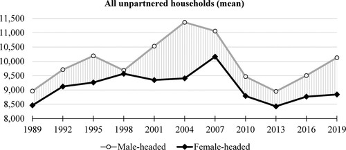
Figure 2 Mean IHS-transformed net wealth of unpartnered male-headed and female-headed households by marital status, 1989–2019

Notes: Shaded area corresponds to the gender wealth gap, calculated as the difference between the IHS-transformed net wealth of male-headed and female-headed households. Values are in natural logarithm units. Real 2019 US dollar values are obtained through the transformation $\sinh \left(y^{IHS}\ast \theta \right)/\theta$ of the mean IHS-transformed wealth (y^IHS); subtracting these dollar values gives the gap in dollars. Unpartnered households only. Source: Author’s calculations based on the US SCF.

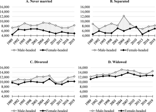
Figure 3 Mean IHS-transformed net wealth of unpartnered male-headed and female-headed households by family structure and race/ethnicity, 1989–2019

Notes: Shaded area corresponds to the gender wealth gap, calculated as the difference between the IHS-transformed net wealth of male-headed and female-headed households. Values are in natural logarithm units. Real 2019 US dollar values are obtained through the transformation $\sinh \left(y^{IHS}\ast \theta \right)/\theta$ of the mean IHS-transformed wealth (y^IHS); subtracting these dollar values gives the gap in dollars. Unpartnered households only. Source: Author’s calculations based on the US SCF.

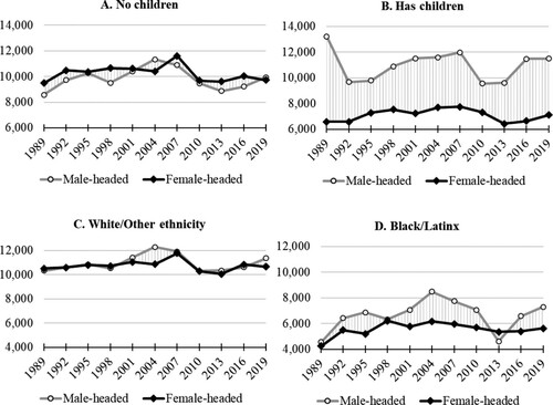
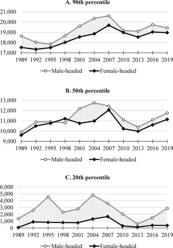
Figure 4 IHS-transformed net wealth of unpartnered male-headed and female-headed households at percentiles of IHS net wealth distribution, 1989–2019

Notes: Shaded area corresponds to the gender wealth gap, calculated as the difference between the IHS-transformed net wealth of male-headed and female-headed households. Values are in natural logarithm units. Real 2019 US dollar values are obtained through the transformation $\sinh \left(y^{IHS}\ast \theta \right)/\theta$ of the mean IHS-transformed wealth (y^IHS); subtracting these dollar values gives the gap in dollars. Unpartnered households only. Source: Author’s calculations based on the US SCF.

There are three visible periods in which the gender wealth gap increased. Firstly, wealth inequality expanded between the 1992 and 1995 survey waves, corresponding to the initial period of recovery from the 1990–91 recession. In this phase, both groups experienced a rise in net wealth, but the increase was higher for unpartnered male-headed households. Secondly, the gender wealth gap rose between the 1998 and 2004 survey waves, suggesting that the initial phase of the subprime lending expansion was associated with rapid increases in the IHS-transformed wealth of male-headed households from 9,690 ($30,372) in 1998 to 11,365 ($50,363) in 2004, but a slight decline in real terms for the female-headed households from 9,566 ($29,300) in 1998 to 9,410 ($27,931) in 2004. Therefore, the gender wealth gap reached its peak of 1,960 ($22,432) in 2004. Lastly, the gender wealth gap grew between 2013 and 2019, implying that the recovery from the Great Recession was not gender equal. In this period, the IHS-transformed wealth of male-headed households increased from 8,950 ($24,313) to 10,130 ($34,712) compared to a slower rise for female-headed households from 8,430 ($20,761) to 8,840 ($23,526). Nevertheless, in 2019 both groups had lower mean wealth holdings than the pre-Great Recession peak values.

In the remaining years of the survey, the gender wealth gap was mostly stagnant, with only two distinct periods of decline. Between 1995 and 1998, mean net wealth of male-headed households fell while the wealth of female-headed households continued to rise, and thus the unconditional wealth gap declined to 120 ($1,073). Similarly, net wealth of male-headed households decreased between 2004 and 2007 compared to an increase for female-headed households in these years, which corresponds to the later stage of the subprime lending boom. In 2007, the gender wealth gap stood at 893 ($10,824), which was lower than its peak observed in 2004, but higher than its value in 1989. Between 2007 and 2013 in the immediate aftermath of the Great Recession, both genders experienced wealth losses to a similar extent.

Differences across marital status

In 2019, 34.7 percent of unpartnered female-headed households in the sample were divorced, 34 percent were never married, 24.8 percent were widowed, and 6.5 percent were separated. In comparison, in 2019 55 percent of unpartnered male-headed households in the sample were never married, 29 percent were divorced, 10.4 percent were widowed, and 5.8 percent were separated. Figure 2 shows trends in mean IHS-transformed net wealth of unpartnered male-headed and female-headed households across the reported marital status. For both genders, never married and separated households had overall the lowest levels of net wealth between 1989 and 2019 compared to the other categories, while the wealth of widowed households was the highest. Divorced households accumulated above-average levels of wealth, particularly among male-headed households. Never married and divorced female-headed households, as well as separated male-headed households, experienced sluggish increases in their net wealth between 1989 and 2019 compared to a steadier growth for the other groups. Nevertheless, wealth holdings of separated, widowed, and divorced households declined substantially between 2007/2010 and 2013 in the aftermath of the Great Recession.

The gender gap in the IHS-transformed wealth was relatively the highest among never married and separated households, although in the latter group it was more volatile. The wealth gap was relatively the smallest among widowed households. In contrast to the post-2001 period, patterns of wealth inequality were less consistent across the categories of marital status before the subprime lending boom. Between 1989 and 1992, the gender wealth gap declined among never married and separated households, but it expanded until 1995 and 1998 respectively before falling again in 2001. Among divorced households, wealth inequality increased between 1989 and 1995, followed by a decrease until 1998. In comparison, widowed households saw a steady fall in the gender wealth gap between 1989 and 1998.

In the years corresponding to the subprime lending expansion, households in all categories of marital status experienced increasing wealth inequality. The gender wealth gap peaked in 2004 for separated, divorced, and widowed households and in 2007 for never married households. At the time of the Great Recession, the gender wealth gap fell across the board. The most sizeable declines are observed for divorced and separated households. For the latter category, the gap briefly turned negative, with 407 ($1,950) higher mean IHS-transformed wealth estimated for separated female-headed households in 2010. However, the gender wealth gap rose between 2013 and 2019 for all categories of marital status apart from separated households, for whom the gap decreased due to faster growth in wealth of female-headed households compared to the male-headed households.

Differences across family structure and race/ethnicity

A greater share of female-headed households in the sample reported having children compared to male-headed households, although the difference decreased over time. At its peak in 2007, 15.7 percent of male-headed households had children compared to 37.4 percent of female-headed households. There are also marked differences in the racial/ethnic composition of male-headed and female-headed households. The share of male-headed households whose head was Black/Latino nearly doubled from 16.6 percent in 1995 to 30.4 percent in 2019. The respective proportion of Black/Latina female-headed households increased from its low of 27.6 percent in 1998 to 36 percent in 2019.

Figure 3 depicts the changes in mean IHS-transformed net wealth of unpartnered male-headed and female-headed households across family structure and by race/ethnicity of household head. In 1989, unpartnered female-headed households with children had 6,650 ($76,286) lower IHS-transformed net wealth than unpartnered male-headed households with children. The gap declined by 1995 but it increased again to over 4,000 (around $40,000) in the 2001–7 survey waves. While the gap fell in the aftermath of the Great Recession between 2007 and 2013 owing to disproportionately greater losses for male-headed households, it expanded between 2013 and 2019, reaching nearly 5,000 (over $40,000). In contrast, female-headed households without children had higher wealth levels than their male-headed counterparts between 1989 and 2001 as well as between 2007 and 2016, although the difference did not exceed 1,000 ($12,000) apart from 1998. In the 2004 and 2019 survey waves, the wealth gap between male-headed and female-headed households without children turned positive in favor of male-headed households.

Moreover, relatively greater disparities in the IHS-transformed wealth are observed for Black/Latinx households in comparison to the White/Other ethnicity households. The gender wealth gap among Black/Latinx households increased between 1989 and 1995, but by 1998 it declined substantially. The gap expanded again in the years of the subprime lending expansion, reaching its peak of 2,310 ($10,765) in 2004. Following the Great Recession, the wealth gap decreased to a negative value in 2013 (indicating higher mean wealth holdings of unpartnered Black/Latina female-headed households) due to steeper wealth losses for the male-headed households. However, by 2019 the gender wealth gap increased in favor of unpartnered Black/Latino male-households to 1,670 ($5,976). Conversely, the gender wealth gap among White/Other ethnicity households was negative albeit relatively small in the 1989 and 1998 survey waves, averaging approximately 83 ($964) in favor of the White/Other ethnicity female-headed households. However, between 2001 and 2013, the gap turned positive, and at its peak in 2004 White/Other ethnicity male-headed households held on average 1,420 ($23,073) more wealth than their female-headed counterparts. By 2007, gender wealth disparities among White/Other ethnicity households largely diminished, although between 2016 and 2019 the gap widened to 710 ($9,690).

Table A2 in the Online Appendix shows that within-group inequality in mean IHS-transformed wealth between households without and with children was relatively higher among female-headed households, peaking at 3,840 ($37,136) in 2007. Male-headed households with children typically had higher mean wealth holdings than households without children. Moreover, the racial gap in the IHS-transformed wealth was higher among female-headed households in most survey years, reaching 5,820 ($47,364) in 2007. This suggests that female-headed unpartnered-parent households and unpartnered Black/Latina female-headed households were particularly disadvantaged in terms of wealth accumulation.

Differences across wealth distribution

Figure 4 depicts trends in the IHS-transformed wealth at the 20th, 50th, and 90th percentile of the IHS-transformed net wealth distribution. Relatively the highest gender gap in the IHS-transformed wealth is observed at the 20th percentile, increasing from 1,300 ($1,340) in 1989 to 2,510 ($2,883) in 2019. The gender wealth gap at the 90th percentile of the distribution was also notable, although it fell overall from 1,108 ($126,270) in 1989 to 466 ($73,876) in 2019. At the 50th percentile, the gender wealth gap was comparatively the smallest, although it expanded over time from 295 ($2,758) in 1989 to 623 ($9,687) in 2019.

Between 1989 and 1995, the gender wealth gap decreased at the 50th and 90th percentile of the IHS-transformed net wealth distribution due to faster wealth increases for female-headed households. However, the gap grew at the 20th percentile, with more rapid wealth accumulation for male-headed households. This was followed by a decline in the gender wealth gap between 1995 and 1998 at the 20th and 50th percentile of the distribution, while the gap began expanding at the 90th percentile.

The survey years corresponding to the subprime lending expansion were paralleled by rising wealth inequality at all examined percentiles of the IHS-transformed net wealth distribution. The gender wealth gap at the 20th percentile rose from 1,500 ($1,684) in 1998 to 3,512 ($5,351) in 2004. In the same period, the gap at the 50th percentile expanded from a negative value of 400 ($5,495) in 1998 to its peak of 1,775 ($31,642). At the 90th percentile, the gender wealth gap increased from 335 ($33,595) in 1995 to 1,506 ($272,100) in 2004. Around the time of the Great Recession, the gap declined, reaching 460 ($464) and 403 ($4,283) at the 20th and 50th percentile respectively in 2013, and falling to a low of 192 ($29,340) at the 90th percentile in 2010. The scale of wealth losses was disproportionately high for male-headed households at the 20th and 90th percentile. However, during the period of recovery in the 2010s, the gender wealth gap increased across the board, particularly at the 20th percentile.

Table A2 in the Online Appendix reveals that for both genders within-group wealth inequality increased between 1992 and 2019, which is driven mainly by low wealth levels at the 20th percentile of the distribution. Relatively larger wealth disparities are observed among female-headed households, with the gap between the 90th and 20th percentile increasing from a low of 16,437 ($301,844) in 1992 to 18,590 ($492,305) in 2019. The difference between the 50th and 20th percentile grew from 9,523 ($29,563) in 1989 to 10,766 ($46,700) in 2019.

Differences in wealth accumulation capacities

To understand how the above trends in wealth inequality changed relative to the factors influencing wealth accumulation, Figures 5–7 depict the evolution of labor market characteristics and the ownership of different types of wealth across gender. Detailed information on the remaining variables is provided in Table A3 in the Online Appendix. On average, female-headed households were older than male-headed households. In contrast to increasing wealth inequality, differences in educational attainment, employment income, and self-employment narrowed down between 1989 and 2019. Nevertheless, Figure 5 shows that substantial differences persisted in labor market characteristics. The employment income gap fell from its high of 2,614 ($10,855) in 1998 to 1,264 ($4,824) in 2019. Similarly, although the proportion of self-employed female-headed households increased since 1989 to 5.2 percent in 2019, the share was more than twice as high for male-headed households that year at 10.8 percent.

Figure 5 Change in labor market characteristics across gender of household head, 1989–2019

Notes: Left-hand side axis: proportion of self-employed households (%). Right-hand side axis: employment income (IHS transformed). Employment income is in natural logarithm; the real 2019 US dollar values can be obtained through the transformation: $\sinh \left(y_{emp}^{IHS}\ast \theta \right)/\theta$. Unpartnered households only. Source: Author’s calculations based on the US SCF.

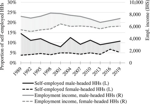
Figure 6 Change in wealth ownership rates across gender of household head, 1989–2019

Notes: Mean proportion of households owning asset. Unpartnered households only. Source: Author’s calculations based on the US SCF.

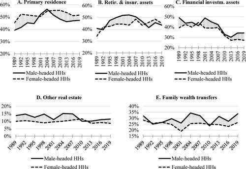
Figure 7 Change in leverage measures across gender of household head, 1989–2019

Notes: Left-hand side axis: debt-to-income ratio (conditional median, %). Right-hand side axis: proportion of households who are sixty-plus days late with debt payments (%). Unpartnered households only. Source: Author’s calculations based on the US SCF.

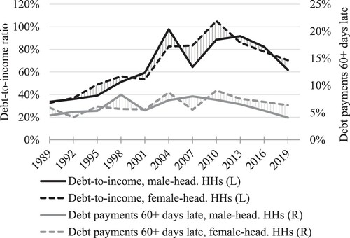
Figure 6 depicts large disparities in asset ownership, some of which increased over time. A greater proportion of female-headed households owned primary residence compared to male-headed households. The homeownership rate peaked at 55.4 percent in 2010 for female-headed households and 56.3 percent in 2004 for male-headed households. Following the Great Recession, homeownership rates fell for both genders, remaining below their earlier peak values at 47.3 percent and 51.6 percent in 2019 for male-headed and female-headed households respectively. Furthermore, differences in the ownership rate of retirement and insurance assets declined over time. Between 1989 and 2010, a greater proportion of male-headed households owned retirement and insurance assets, but between 2013 and 2019, the ownership rate was higher for female-headed households. In 2007, when the ownership rate was the highest for both groups, 50.6 percent of male-headed households and 48.5 percent of female-headed households owned retirement and insurance assets, but the ownership rates fell to 43.5 percent and 45 percent respectively in 2019.

In contrast, the ownership rate of other real estate and financial investment assets as well as access to FWT remained decidedly unequal. At the peak in 2007, 15 percent of male-headed households owned other real estate, compared to 10.8 percent of female-headed households. In 2019, the ownership rate of other real estate fell to 11.4 percent and 8.6 percent respectively. Moreover, the difference in the ownership rate of financial investment assets stood at 10 percentage points in 1989, and while it largely narrowed down by 2010, it increased thereafter. In 2019, 34.3 percent of male-headed households held financial investment assets compared to 27.2 percent of female-headed households. Furthermore, a greater share of male-headed than female-headed households had access to FWT. Except for 2010, the difference in this proportion increased between 1998 and 2019, reaching 33.7 percent and 26.4 percent among male-headed and female-headed households respectively in 2019.

Figure 7 shows higher relative indebtedness for female-headed households than male-headed households. The conditional median value of the debt-to-income ratio increased from 32.7 percent in 1989 to a peak of 105.1 percent in 2010 for female-headed households, reaching 70.3 percent in 2019. For male-headed households, the ratio rose from 33.6 percent in 1989 to 97.8 percent in 2004, falling to 61.8 percent in 2019. Moreover, at its peak, 9 percent of female-headed households were more than sixty days late with debt repayments in 2010, compared to 8 percent of male-headed households in 2007. By 2019, the proportion reached 6.4 percent and 4 percent for each group respectively, representing an overall increase in the share for female-headed households but a decline for male-headed households since the 1990s.

Tables A4–A9 in the Online Appendix show that among households with children, Black/Latinx households, and across marital status, gender differences were broadly consistent with the patterns for all unpartnered households. Nevertheless, disparities across these categories were notable. Wealth ownership rates were typically lower for separated and never married households and higher among widowed households, while employment income was on average higher for never married households and lower for widowed households (Tables A4–A7). A greater share of separated households and never married female-headed households were Black/Latinx. Moreover, female-headed households with children were younger than their male-headed counterparts, with substantially lower wealth ownership rates (Table A8). A relatively greater proportion of female-headed households with children were Black/Latina and reported being late with debt repayments. Similarly, more Black/Latina female-headed households had children and fewer were self-employed compared to Black/Latino male-headed households (Table A9). There were also large gender disparities in this group in employment income and the ownership of other real estate, financial investment assets, and FWT. Nevertheless, Black/Latinx households had substantially lower wealth ownership rates compared to the overall mean for unpartnered households, especially for primary residence, financial investment assets, and FWT.

The above analysis does not examine the statistical significance of the gender wealth gap or the impact of changes in factors influencing wealth accumulation. Instead, it provides an in-depth examination of differences in these factors and their change over time in light of the institutional changes in the US economy. The largest gender disparities are observed for variables related to wealth composition, relative indebtedness, employment income, race/ethnicity, marital status, and family structure. The widening of the overall gender wealth gap between 1998 and 2004 was paralleled by increasing disparities in the ownership rates of real estate, retirement and insurance assets, financial investment assets, and access to FWT as well as persistent gaps in employment income. Between 2004 and 2007 wealth accumulation was relatively higher for female-headed households. The Great Recession led to wealth losses for both genders, but they were relatively steeper for male-headed households who were divorced, with children, Black/Latinx, and at the 20th or 90th percentile of wealth distribution. However, after the crisis wealth of male-headed households recovered more quickly across the board compared to female-headed households.

Inequality decomposition

We estimate the statistical significance of the IHS-transformed gender wealth gap at the 1, 5, and 10 percent level conditional on the factors influencing wealth accumulation. Figure 8 shows the total, explained, and unexplained conditional gender wealth gap estimated using the mean-based OB and the OB-RIF decomposition.²⁴ Table A10 in the Online Appendix provides standard errors of these estimates.

Figure 8 Conditional gender gap in IHS-transformed net wealth, 1989–2019

Notes: Striped bars of “Unexplained gap” and “Explained gap” and markers of “Total gap” without fill denote estimates that are not statistically significant at 1, 5, or 10 percent level. Estimates are obtained from the mean-based Oaxaca-Blinder decomposition based on a pooled OLS regression (panel A) and the Oaxaca-Blinder decomposition based on a RIF regression (panels B-D). Values are in natural logarithm; the real 2019 US dollar values can be obtained by subtracting the dollar values of wealth of male-headed and female-headed households (obtained through the transformation of the IHS wealth values: $\sinh \left(y^{IHS}\ast \theta \right)/\theta$). Unpartnered households only. Source: Author’s calculations based on the US SCF.

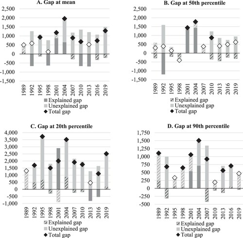
At all analyzed points of the IHS-transformed net wealth distribution, the magnitudes of the conditional gender wealth gap are consistent with the values presented in Figures 1 and 4. The mean conditional gender wealth gap is estimated to be statistically significant in 1995 as well as between 2001–10 and 2016–19. The conditional gap at the 20th percentile of the distribution is found to be statistically significant in all survey years apart from 1989 to 2013. At the median, the conditional gap tends not to be statistically significant except for the 2001, 2004, and 2010 survey years. The conditional gender wealth gap at the 90th percentile is statistically significant between 1989–92, 1998–2007, and 2013–16.

At all analyzed points of the distribution, the conditional gender wealth gap is estimated to arise primarily due to unexplained differences in the estimated coefficients. The unexplained gap is positive and statistically significant in the majority of years. The explained wealth gap tends to be the most consistently significant at the mean of the distribution, and its contribution is generally negative, turning positive in 2001 and 2004. At the 20th, 50th, and 90th percentile of the distribution, the explained gap is statistically significant in selected years corresponding to the subprime lending boom, when it tends to be positive, as well as at the 20th percentile after the Great Recession, when it is negative.

The estimated contributions of factors influencing wealth accumulation are found to be statistically significant, primarily in terms of the explained portion of the gender wealth gap. Figure 9 illustrates the detailed contribution of selected variables to the explained conditional gender wealth gap in the mean-based OB decomposition. Complete results with standard errors are given in Table A11 in the Online Appendix. Detailed results of the OB-RIF decomposition are in Tables A12–A14, while Table A15 depicts the correlation matrix. Variables that are estimated to have the most consistent statistically significant contribution to the explained wealth gap are employment income, age, household head being Black/Latinx, household head being self-employed, as well as ownership of primary residence and retirement and insurance assets. The contribution to the explained wealth gap of differences in employment income and self-employment was positive, but its magnitude declined between 1989 and 2019. The contribution of differences in wealth due to household head being Black/Latinx was also positive, rising between 1989 and 2001 and between 2004 and 2016. The ownership of retirement and insurance assets had a positive and increasing contribution to the explained wealth gap between 1989 and 2001, but the contribution fell between 2001 and 2010, turning negative between 2013 and 2019.

Figure 9 Contribution to the explained conditional gender wealth gap, mean-based OB decomposition, 1989–2019

Notes: Bars only shown for statistically significant estimates at 1, 5, or 10 percent level. FWT: family wealth transfers. Dependent variable: IHS-transformed net wealth. Values in natural logarithm units. Unpartnered households only. Source: Author’s calculations based on the US SCF.

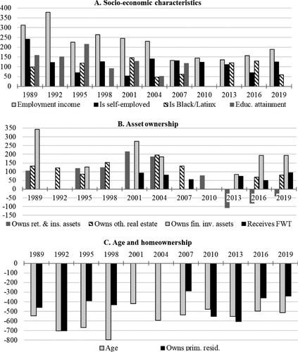
Moreover, it is estimated that differences in age and the ownership of primary residence contributed negatively to the explained wealth gap. The contribution of differences in age was on average the highest in absolute terms between 1989 and 1998. This can be understood by the observation made in Table A3 in the Online Appendix that unpartnered female-headed households in the sample tend to be on average older and have higher homeownership rates than unpartnered male-headed households. Because of these higher observed values, the estimated contribution of age and the ownership of primary residence to the explained wealth gap is negative. However, it is notable that the contribution of the ownership of primary residence was estimated not to be statistically significant in the years of the subprime lending boom in 2001 and 2004. This can be explained by comparatively higher increases in the average homeownership rate for unpartnered male-headed households compared to unpartnered female-headed households in these years (Table A3 in the Appendix).

Furthermore, the ownership of other real estate and financial investment assets contributed positively to the explained wealth gap, increasing in magnitude between 1995 and 2001/2004. While the contribution of these factors was not statically significant around the time of the Great Recession, it regained significance and increased in size by 2019. Similarly, differences in the explained wealth gap due to the household being more than sixty days late with debt repayments became positive and statistically significant in 2010, 2016, and 2019. In addition, the contribution of access to FWT, while relatively small, turned positive and statistically significant between 2001 and 2019 (apart from 2010). Differences in educational attainment contributed positively to the explained wealth gap between 1989 and 2007, but the estimate lost its statistical significance between 2010 and 2019.

The unexplained part of the gender wealth gap is estimated to have a less consistent contribution from the analyzed variables. Differences in the coefficients of employment income contributed positively to the unexplained gap in 1998, 2004, and between 2016–19. The contribution of differences in the coefficients for the ownership of primary residence was negative but statistically significant only in 1989, 1998, 2004–7, and 2019. The relevant estimates for the remaining variables were statistically significant in fewer than four survey waves.

The statistical significance and magnitudes of the estimates are broadly consistent at different points of the IHS-transformed net wealth distribution. It is noteworthy that at the 20th percentile, the contributions of differences in age, educational attainment, and self-employment to the explained wealth gap were less significant than at the mean and median of the distribution, while differences due to race contributed relatively more. Moreover, differences in the estimated coefficients of the ownership of primary residence and retirement and insurance assets contributed positively to the unexplained wealth gap at the 20th percentile in the years of the subprime period. Conversely, at the 90th percentile, differences across race contributed comparatively less to the explained gender wealth as did differences in employment income, age, and ownership of retirement and insurance assets.

Comparing our findings to the literature, similarly to Laura Ravazzini and Jenny Chesters (2019) we find a significant role of housing wealth and the gender pay gap in explaining gender wealth inequality; however, the impact of education is lower in our sample. In contrast to Alyssa Schneebaum et al. (2018), who establish a significant gender wealth gap primarily at the top of the distribution, we find a substantial and significant conditional gender wealth gap primarily towards the bottom of the distribution. Moreover, we do not find consistent evidence that pension transformation had a disproportionately negative impact on wealth of female-headed households; this effect is only observed between 1995 and 2004.

The inconsistency of the estimates in the detailed decomposition of the unexplained gap does not immediately suggest that there are no significant differences across gender in the estimated returns to the factors influencing household wealth accumulation, particularly given that the unexplained gap is overall statistically significant. Rather, this highlights the challenges to temporal analyses of the gender wealth gap posed by the dataset’s complexity, multiply imputed structure, and unbalanced sample size across household groups and over time. In this light, the descriptive and conditional analyses should be seen as complementary tools, each displaying its own merits and limitations in understanding trends in household wealth inequality. Future research will extend this approach to a detailed examination of wealth inequality and its determinants at the intersection of gender, race, family structure, and marital status.

CONCLUSION

The original contribution of this article is to analyze the patterns of gender wealth inequality across unpartnered households in the US, particularly in the context of institutional changes arising from securitization, the subprime lending expansion, and broader liberalization policies. The study provides new insights into understanding the extent of the gender wealth inequality across households with different characteristics and its changes over time. The magnitude of wealth disparities between unpartnered male-headed and female-headed households was found to vary substantially across the categories of marital status, family structure, and race/ethnicity of household head. Substantial within-group inequality was also established among female-headed households. However, despite this heterogeneity, the years of the subprime lending boom, particularly its initial phase, were associated with the widening of the gender wealth gap across all these categories of unpartnered households.

Moreover, the article finds that female-headed households saw overall modest increases in their net wealth in real terms between 1989 and 2019. This is primarily owing to slow wealth accumulation after the Great Recession, although the wealth of never married and Black/Latina female-headed households declined in real terms since the early years of the subprime lending boom. While the Great Recession was paralleled by wealth losses for both genders and reductions in wealth disparities, inequality increased during the time of recovery recorded between the 2013 and 2019 survey years. In some instances, at the end of the analyzed period, the gender wealth gap was approaching or even exceeded its peak value from the subprime era, particularly among never married households and households with children. This paints a worrying picture for the financial fragility of female-headed households on the eve of the COVID-19 pandemic, particularly those who are never married, with children, Black/Latina, or toward the bottom of the distribution.

Furthermore, the study used recent methodological developments and applied the OB-RIF decomposition to examine the extent of wealth inequality at different points of the wealth distribution. The gender wealth gap for unpartnered households was found to be relatively the largest and the most consistently significant at the 20th percentile, and to some extent at the 90th percentile of the distribution. The inequality decomposition analysis also established that the contribution of factors affecting household wealth accumulation differed somewhat at the 20th and 90th percentile compared to the mean-based OB decomposition. Differences in age appeared to play a smaller role in explaining the gender wealth gap at the extremes of the wealth distribution.

The article suggests potential areas of policy action to alleviate gender wealth inequality. Decomposition of the conditional gender wealth gap established that the observed gender differences in employment income, age, self-employment, and race/ethnicity explain some degree of gender wealth inequality. Therefore, reducing gender disparities in employment income and self-employment has potential to alleviate the gender wealth gap, by boosting the capacity to save among female-headed households.

We also find that decreasing disparities in educational attainment and the ownership of retirement and insurance assets, which were established in the descriptive analysis, were paralleled by a reduction in the contribution of these variables to the gender wealth gap. This indicates that expanding the ownership of the more unequally distributed high-yielding assets as well as access to FWT could improve wealth accumulation for female-headed households. Differences in homeownership were estimated to reduce the gender wealth gap, although in the subprime years the otherwise equalizing effect of the ownership of primary residence lost its statistical significance. Given the disparities in homeownership across female-headed households with different characteristics, broadening access to homeownership and ensuring its resilience to the business cycle are shown to be instrumental in alleviating the gender wealth inequality.

ACKNOWLEDGMENTS

I am grateful to the Editor and four anonymous reviewers for their detailed and helpful comments. I would like to thank Diego A. Quinones Valles for his advice and support, as well as the Gender and Working Lives writing group for creating a friendly and productive space to develop this paper.

Additional information

Notes on contributors

Hanna K. Szymborska

Hanna K. Szymborska is Senior Lecturer in Economics at Birmingham City University, UK. Her research interests include economics of inequality, household finance, financial macroeconomics, and history of economic thought. She has previously worked as a lecturer in economics at The Open University UK, teaching assistant at the University of Leeds, assistant economist at the UK Department of Health, and research assistant at SOAS, University of London and at London School of Economics and Political Science.

Notes

1 While modern securitization emerged as early as 1960s, implementation of financial deregulation legislation in the 1990s led to a debt securitization boom in the early 2000s, particularly in mortgage-backed securities (Buchanan 2017). This was facilitated by the re-emergence of investment banking activity and the extension of mortgages to subprime borrowers, whose access to credit had been previously constrained. Low-income individuals, women, people of color, and women of color were disproportionately represented among the subprime borrowers (Phillips 2012). Debt securitization allowed financial institutions to move the loan default risk off their balance sheets, simultaneously generating high profits from securities underwriting fees. Because subprime mortgage-holders faced higher loan repayment rates and harsher penalties than prime borrowers, wealth accumulated by subprime homeowners in the 2000s was highly leveraged (Dymski, Hernandez, and Mohanty 2013).

2 A household is defined as an economically dominant individual (unpartnered) or a couple over 17 years old, together with all financially dependent individuals (Federal Reserve 2019a).

3 Net wealth is defined based on self-reported values of assets and debt at the time of the interview. Assets include: transaction accounts, savings accounts, retirement and insurance assets, high-yielding financial assets, property wealth, business equity, vehicles, and consumer durables. Liabilities include: secured debt and unsecured debt (instalment loans, credit card debt, and other). While vehicles and consumer durables are sometimes excluded from the definition of household wealth (Wolff 2017: 46), such exclusion in the context of gender may risk artificial lowering of the extent of inequality. Vehicles and consumer durables are not conducive to saving and long-term growth in wealth because they yield negative returns over time, compared to positive returns from ownership of real estate or financial assets. However, these low-yielding forms of wealth typically constitute a substantial portion of women’s asset portfolios (Sierminska 2018).

4 The IHS transformation is a logarithmic-style transformation based on the following equation, where parameter θ denotes the degree of linearity of a y function (the closer θ is to zero, the more linear the function is for a larger proportion of its domain): ${\theta }^{-1}{\sinh }^{-1}\left(\theta y\right)={\theta }^{-1}\ln \left(\theta y+{\left({\theta }^2{y}^2+1\right)}^{1/\phantom{12}2}\right)$. Based on Pence (2006), we assume θ = 0.0003. The IHS-transformed. values of wealth are expressed in natural logarithm units. The advantage of this approach is that it allows to scale the data in a way that enhances the visibility of wealth disparities at small values of wealth holdings, which are prevalent at some of the analyzed household categories.

5 This is a common practice in the literature, see Maury Gittleman and Edward N. Wolff 2004; Lucie Schmidt and Purvi Sevak 2006.

6 Due to data limitations, we are only able to unambiguously distinguish between four racialized groups: White, Black, Latinx, and Other ethnicity. The latter category groups households whose head is Asian American, American Indian, Alaska Native, Native Hawaiian/Pacific Islander, or other. A shortcoming of this approach is that we are not able to reliably analyse wealth holdings of Asian American households because too few of them were surveyed in any individual year of the US SCF (Weller and Thompson 2016). Available evidence shows that there was substantial change in finances of Asian Americans between 1970 and 2016, with particularly high increases in within-group inequality by the mid-2010s (Kochhar and Cilluffo 2018; Weller and Thompson 2016).

7 Educational attainment is measured as an index of the highest educational achievement of household head, ranging from 1 (no grades completed) to 17 (completed graduate school). Age effects include age of household head and its squared term.

8 The public version of the US SCF excludes geographical characteristics of a household. The subsequent analysis is therefore unable to control for regional differences in wealth accumulation.

9 Such comparison of the racialized groups (White/Other ethnicity versus Black/Latinx) is motivated by disparities in the IHS-transformed net wealth ratios between these four categories. Among unpartnered female-headed households, the ratio of the median IHS-transformed net wealth in 2019 stood at 2.5 between White and Black households (6.7 in 1989), 2.2 between White and Latina households (15.8 in 1989), and 0.8 between White and Other ethnicity households (1.6 in 1989; author’s calculations based on the US SCF).

10 Employment income is measured before transfers and taxes for the calendar year prior to the survey wave. The variable is IHS-transformed to maintain consistency with the measurement of wealth.

11 While other labor market characteristics may matter for women’s wealth (for example, labor force participation, working hours), these are highly correlated with employment income in the dataset.

12 Other real estate includes residential and non-residential property. Financial investment assets include certificates of deposits, savings bonds, bonds, stocks, other managed assets, pooled investment funds, and non-money market mutual funds.

13 The debt-to-income ratio is measured on an annual basis and illustrates more long-term indebtedness issues, while the dummy variable for delinquency relates to monthly debt repayments and is reflective of more immediate leverage problems.

14 Retirement and insurance assets include Individual Retirement Accounts, Keogh accounts, 401(k), and other retirement accounts, and the cash value of life insurance plans.

15 The IHS-transformed net wealth (y^IHS) is in natural logarithm units, with real 2019 US dollar values given in parentheses. The latter are obtained using the transformation: $\sinh \left(y^{IHS}\ast \theta \right)/\theta$.

16 This is implemented in Stata using the user-written program oaxaca (Jann 2008). The OB decomposition is widely applied in the literature on gender inequality (Daymont and Andrisani 1984; Kim 2009; Sierminska 2018).

17 Design of the US SCF as a multiply imputed repeated cross-section complicates the error term structure in a way that prevents straightforward application of estimation methods typically used to deal with non-spherical errors (fixed/random effects models, autoregressive models, general method of moments models). The OLS estimation is preferred due to its methodological clarity, although we acknowledge its limitations arising from issues with the error term distribution.

18 The estimated contributions of dummy variables are normalized so that they are not affected by the choice of the base category (Jann 2008).

19 We follow the recommendation made by Jann (2008) and take coefficients from a pooled regression including a dummy variable for gender as estimates for the reference coefficients ${\text{β}}_k^{\ast }$. Thus, we do not assume that the coefficients of the male-headed households’ regression are non-discriminating.

20 A three-way decomposition can be performed to include an interaction term between the estimated differences in the observed characteristics and coefficients (Daymont and Andrisani 1984). Due to a limited intuitive interpretation of the interaction term in the present context, a two-way decomposition is selected.

21 This is implemented using the user-written Stata command oaxaca_rif (Rios-Avila 2020).

22 The OB-RIF decomposition is preferred here to other non-mean-based decomposition techniques: It is more widely applied in the literature than the quantile regression-based counterfactual decomposition and allows for a more detailed examination of the contribution of covariates to inequality than the DiNardo, Fortin, and Lemieux decomposition (Rios-Avila 2020).

23 According to Robert Barsky et al. (2002), a counterfactual ${\text{β}}_k^{\ast }$ based on linear estimates may be unreliable if the conditional expected wealth function is non-linear. A reweighting factor can be employed using a logit/probit estimation, measuring the conditional probability of an observation with given characteristics belonging to group 1. The complex structure of the dataset over multiple survey waves renders the reweighting mechanism less transparent in this analysis due to the computational complexity of that approach. We use the conditional expected wealth function of male-headed households to approximate wealth of female-headed households in the OB-RIF decomposition. A limitation of this approach is that we need to assume a linear functional form of the relationship between wealth and the covariates and that variables omitted by the model are distributed independently from the regressors. Nevertheless, in additional analyses using the reweighting approximation in a logit estimation (not reported here), the statistical significance and signs of the estimated contributions to the total wealth gap were largely consistent across the two approaches. Future research focused on a cross-sectional analysis will consider a non-parametric estimation of the counterfactual in the OB-RIF decomposition.

24 Based on Equation 1, statistical significance is determined individually for each element of the wealth gap (total, explained, unexplained) and for each covariate, based on the estimation of bootstrap standard errors with replicate weights. Hence, components of the gender wealth gap may be statistically significant even if the total gap is not statistically significant.

References

- Aloni, Erez. 2018. “The Marital Wealth Gap.” Washington Law Review 93(1): 1–72.
- Anglade, Boaz, Pilar Useche, and Carmen Diana Deere. 2017. “Decomposing the Gender Wealth Gap in Ecuador.” World Development 96: 19–31.
- Arestis, Philip, Aurélie Charles, and Giuseppe Fontana. 2013. “Financialization, the Great Recession, and the Stratification of the US Labor Market.” Feminist Economics 19(3): 152–80.
- Atkinson, Anthony B. and Andrea Brandolini. 2013. “On the Identification of the Middle Class.” In Income Inequality: Economic Disparities and the Middle Class in Affluent Countries, edited by Janet C. Gornick and Markus Jäntti, 77–100. Stanford: Stanford University Press.
- Austen, Siobhan, Therese Jefferson, and Rachel Ong. 2014. “The Gender Gap in Financial Security: What We Know and Don't Know about Australian Households.” Feminist Economics 20(3): 25–52.
- Barsky, Robert, John Bound, Kerwin Kofi Charles, and Joseph P. Lupton. 2002. “Accounting for the Black–White Wealth Gap: A Nonparametric Approach.” Journal of the American Statistical Association 97(459): 663–73.
- Bernasek, Alexandra and Stephanie Shwiff. 2001. “Gender, Risk, and Retirement.” Journal of Economic Issues 35(2): 345–56.
- Blau, Francine D. and John W. Graham. 1990. “Black-White Differences in Wealth and Asset Composition.” Quarterly Journal of Economics 105(2): 321–39.
- Blinder, Alan S. 1973. “Wage Discrimination: Reduced Form and Structural Estimates.” Journal of Human Resources 8(4): 436–55.
- Brewer, Rose M., Cecilia A. Conrad, and Mary C. King. 2002. “The Complexities and Potential of Theorizing Gender, Caste, Race, and Class.” Feminist Economics 8(2): 3–17.
- Brown, Tyson. 2012. “The Intersection and Accumulation of Racial and Gender Inequality: Black Women’s Wealth Trajectories.” Review of Black Political Economy 39(2): 239–58.
- Brown, Jeffrey R., Courtney C. Coile, and Scott J. Weisbenner. 2010. “The Effect of Inheritance Receipt on Retirement.” Review of Economics and Statistics 92(2): 425–34.
- Buchanan, Bonnie G. 2017. “The Way We Live Now: Financialization and Securitization.” Research in International Business and Finance 39(Part B): 663–77.
- Burbidge, John B., Lonnie Magee, and A. Leslie Robb. 1988. “Alternative Transformations to Handle Extreme Values of the Dependent Variable.” Journal of the American Statistical Association 83(401): 123–7.
- Daymont, Thomas N. and Paul J. Andrisani. 1984. “Job Preferences, College Major, and the Gender Gap in Earnings.” Journal of Human Resources 19(3): 408–28.
- Deere, Carmen Diana and Cheryl R. Doss. 2006. “The Gender Asset Gap: What Do We Know and Why Does It Matter?” Feminist Economics 12(1–2): 1–50.
- Denton, Margaret and Linda Boos. 2007. “The Gender Wealth Gap: Structural and Material Constraints and Implications for Later Life.” Journal of Women & Aging 19(3–4): 105–20.
- Dymski, Gary, Jesus Hernandez, and Lisa Mohanty. 2013. “Race, Gender, Power, and the US Subprime Mortgage and Foreclosure Crisis: A Meso Analysis.” Feminist Economics 19(3): 124–51.
- Estes, Carroll L. 2004. “Social Security Privatization and Older Women: A Feminist Political Economy Perspective.” Journal of Aging Studies 18: 9–26.
- Federal Reserve. 2019a. “Codebook for 2019 Survey of Consumer Finances.” Federal Reserve. https://www.federalreserve.gov/econres/files/codebk2019.txt.
- Federal Reserve. 2019b. “U.S. Survey of Consumer Finances, 1989–2019.” Federal Reserve. http://www.federalreserve.gov/econresdata/scf/scfindex.htm.
- Gittleman, Maury and Edward N. Wolff. 2004. “Racial Differences in Patterns of Wealth Accumulation.” Journal of Human Resources 39(1): 193–227.
- Hamilton, Barton H. 2000. “Does Entrepreneurship Pay? An Empirical Analysis of the Returns to Self-Employment.” Journal of Political Economy 108(3): 604–31.
- Hillesland, Marya. 2019. “Investigating the Gender Wealth Gap in Ghana.” Oxford Development Studies 47(1): 63–78.
- Hipple, Steven F. 2010. “Self-Employment in the United States.” Monthly Labor Review, Bureau of Labor Statistics, 17–32.
- Hundley, Greg. 2001. “Why Women Earn Less Than Men in Self-Employment.” Journal of Labor Research 22: 817–29.
- Jann, Ben. 2008. “The Blinder-Oaxaca Decomposition for Linear Regression Models.” Stata Journal 8(4): 453–79.
- Kim, Marlene. 2009. “Race and Gender Differences in the Earnings of Black Workers.” Industrial Relations 48(3): 466–88.
- Kochhar, Rakesh and Anthony Cilluffo. 2018. “Income Inequality in the U.S. Is Rising Most Rapidly Among Asians.” Pew Research Center Inequality Report, July 12.
- Long, Melanie G. 2018. “Pushed into the Red? Female-Headed Households and the Pre-Crisis Credit Expansion.” Forum for Social Economics 47(2): 224–36.
- MacDonald, Martha, Shelley Phipps, and Lynn Lethbridge. 2005. “Taking Its Toll: The Influence of Paid and Unpaid Work on Women's Well-Being.” Feminist Economics 11(1): 63–94.
- Meer, Jonathan, Douglas L. Miller, and Harvey S. Rosen. 2003. “Exploring the Health-Wealth Nexus.” Journal of Health Economics 22: 713–30.
- Mjøset, Lars and Trond Petersen. 1983. “Class and Gender: A Note on Class Structure in Norway and USA.” Acta Sociologica 26(1): 49–60.
- Munnell, Alicia H. and Annika Sundén. 2004. Coming Up Short: The Challenge of 401(k) Plans. Washington, DC: Brookings Institution Press.
- Nakajima, Makoto. 2013. “The Diverse Impacts of the Great Recession.” Philadelphia Fed Business Review Q 2: 17–29.
- Nembhard, Jessica Gordon and Kris Marsh. 2012. “Wealth Affirming Policies for Women of Color.” Review of Black Political Economy 39(3): 353–60.
- Oaxaca, Ronald. 1973. “Male–Female Wage Differentials in Urban Labor Markets.” International Economic Review 14(3): 693–709.
- O’Rand, Angela M. and Kim M. Shuey. 2007. “Gender and the Devolution of Pension Risks in the US.” Current Sociology 55(2): 287–304.
- Pahl, Jan. 2001. “Couples and Their Money: Theory and Practice in Personal Finances.” In Social Policy Review 13. Developments and Debates 2000–2001, edited by Robert Sykes, Catherine Bochel, and Nick Ellison, 17–38. Bristol: Policy Press.
- Pence, Karen M. 2006. “The Role of Wealth Transformations: An Application to Estimating the Effect of Tax Incentives on Saving.” Contributions to Economic Analysis & Policy 5(1): 1–24.
- Percheski, Christine and Christina Gibson-Davis. 2017. “Family Structure & Wealth Inequality among Families with Children, 1989-2013.” http://www.ecineq.org/ecineq_nyc17/FILESx2017/CR2/p190.pdf.
- Peterson, Janice. 2012. “The Great Crisis and the Significance of Gender in the U.S. Economy.” Journal of Economic Issues 46(2): 277–90.
- Pfeffer, Fabian T., Robert F. Schoeni, Arthur Kennickell, and Patricia Andreski. 2016. “Measuring Wealth and Wealth Inequality: Comparing Two U.S. Surveys.” Journal of Economic and Social Measurement 41(2): 103–20.
- Phillips, Sandra. 2012. “The Subprime Mortgage Calamity and the African American Woman.” Review of Black Political Economy 39(2): 227–37.
- Piketty, Thomas. 2014. Capital in the Twenty First Century. Cambridge, MA: Harvard University Press.
- Ravazzini, Laura and Jenny Chesters. 2018. “Inequality and Wealth: Comparing the Gender Wealth Gap in Switzerland and Australia.” Feminist Economics 24(4): 83–107.
- Rios-Avila, Fernando. 2020. “Recentered Influence Functions (RIFs) in Stata: RIF Regression and RIF Decomposition.” Stata Journal 20(1): 51–94.
- Schmidt, Lucie and Purvi Sevak. 2006. “Gender, Marriage, and Asset Accumulation in the United States.” Feminist Economics 12(1–2): 139–66.
- Schneebaum, Alyssa, Miriam Rehm, Katharina Mader, and Katarina Hollan. 2018. “The Gender Wealth Gap across European Countries.” Review of Income and Wealth 64(2): 295–331.
- Sierminska, Eva. 2018. “The ‘Wealth-Being’ of Single Parents.” In The Triple Bind of Single-Parent Families, edited by Rense Nieuwenhuis and Laurie C. Maldonado, 51–80. Bristol: Policy Press.
- Sierminska, Eva, Joachim R. Frick, and Markus M. Grabka. 2010. “Examining the Gender Wealth Gap in Germany.” Oxford Economic Papers 62(4): 669–90.
- Sierminska, Eva and Anastasia Girshina. 2017. Wealth and Gender in Europe. European Commission, Directorate-General for Justice and Consumers Report. https://publications.europa.eu/en/publication-detail/-/publication/c02def1c-92ae-11e7-b92d-01aa75ed71a1/language-en.
- Szymborska, Hanna Karolina. 2019. “Wealth Structures and Income Distribution of US Households Before and After the Great Recession.” Structural Change and Economic Dynamics 51: 168–85.
- Warren, Tracey. 2006. “Moving Beyond the Gender Wealth Gap: On Gender, Class, Ethnicity, and Wealth Inequalities in the United Kingdom.” Feminist Economics 12(1–2): 195–219.
- Weller, Christian E. and Jeffrey Thompson. 2016. “Wealth Inequality among Asian Americans Greater Than Among Whites.” Center for American Progress Report, December.
- Wilmoth, Janet and Gregor Koso. 2002. “Does Marital History Matter? Marital Status and Wealth Outcomes among Preretirement Adults.” Journal of Marriage and Family 64(1): 254–68.
- Wolff, Edward N. 2017. A Century of Wealth in America. Cambridge, MA: Harvard University Press.
- Wolff, Edward N. and Ajit Zacharias. 2013. “Class Structure and Economic Inequality.” Cambridge Journal of Economics 37(6): 1381–406.
- Yamokoski, Alexis and Lisa A. Keister. 2006. “The Wealth of Single Women: Marital Status and Parenthood in the Asset Accumulation of Young Baby Boomers in the United States.” Feminist Economics 12(1–2): 167–94.
- Young, Brigitte. 2010. “The Gendered Dimension of Money, Finance and the Subprime Crisis.” In Gender and Economics. Feministische Kritik der politischen Oekonomie, edited by C. Bauhardt and G. Caglar, 258–77. Wiesbaden: VS Verlag für Sozialwissenschaften.