A comparison of the B-spline group-based trajectory model with the polynomial group-based trajectory model for identifying trajectories of depressive symptoms around old-age retirement

Abstract

Objectives: The life event of retirement may be associated with changes in levels of depressive symptoms. The use of polynomial group-based trajectory modelling allows any changes to vary between different groups in a sample. A new approach, estimating these models using B-splines rather than polynomials, may improve modelling of complex changes in depressive symptoms at retirement.

Methods: The sample contained 1497 participants from the Swedish Longitudinal Occupational Survey of Health (SLOSH). Polynomial and B-spline approaches to estimating group-based trajectory models were compared.

Results: Polynomial group-based trajectory models produced unexpected changes in direction of trajectories unsupported by the data. In contrast, B-splines provided improved insights into trajectory shapes and more homogeneous groups. While retirement was associated with reductions in depressive symptoms in the sample as a whole, the nature of changes at retirement varied between groups.

Conclusions: Depressive symptoms trajectories around old age retirement changed in complex ways that were modelled more accurately by the use of B-splines. We recommend estimation of group-based trajectory models with B-splines, particularly where abrupt changes might occur. Improved trajectory modelling may support research into risk factors and consequences of major depressive disorder, ultimately assisting with identification of groups which may benefit from treatment.

Keywords:

• B-spline smoothing
• depressive symptoms
• group-based trajectory models
• polynomial fitting
• old-age retirement

Introduction

Major depressive disorder is highly prevalent worldwide (Vos et al., 2017). Depressive symptoms are common among older people and have been associated with reduced quality of life (Blazer, 2003), dementia risk (Modrego & Ferrández, 2004) and higher mortality (Bogner, Morales, Reynolds, Cary, & Bruce, 2012).

A consensus is growing about the importance of integrating a life course perspective into mental health research, with one area of interest being the influence of life events upon the development of illness (Amick, McLeod, & Bültmann, 2016; Colman & Ataullahjan, 2010; Heikkinen, 2011). Retirement is an important social transition of late adulthood, and thereby has potential mental health consequences, since retirement can disrupt social support networks but may also terminate exposure to stressful working conditions. Traditional statistical approaches, such as hierarchical linear modeling (Goldstein, 2010; Raudenbush & Bryk, 2001) and latent curve analysis (Muthén, 1989), have as a starting point that individuals will follow the same developmental trajectory. Studies using such approaches to assess changes in psychological health at retirement identify the average trend over time and quantify the degree of individual variation around this estimate (Jokela et al., 2010; Leinonen, Lahelma, & Martikainen, 2013; Oksanen et al., 2011; Vahtera et al., 2009; Westerlund et al., 2010; Zins et al., 2011).

However, some studies have demonstrated variability in the reaction to retirement (Pinquart & Schindler, 2007; Wang, 2007), highlighting the need to examine the course of depressive symptoms in a way that enables the study of groups with differing trajectories of depressive symptoms (Andreescu, Chang, Mulsant, & Ganguli, 2008; Henning, Lindwall, & Johansson, 2016; Lindwall et al., 2017). Group-based trajectory models allow study of such heterogeneity (Nagin, 1999, 2005). These methods are widely used in epidemiology, providing opportunities to examine and model the course as well as variations over time of various disorders using symptoms-based data (Kwon, Kim, Lee, & Park, 2017; Musliner, Munk-Olsen, Eaton, & Zandi, 2016; Peristera, Westerlund, & Magnusson Hanson, 2018). They have become popular approach to analyze developmental trajectories since they allow trends to be summarized in a convenient way and variability between trajectories to be described. These methods can also be used to analyze potential predictors and consequences of developmental trajectories.

Group-based trajectory models assume that the underlying population consists of a fixed but unknown number of groups, which have distinct trajectories. These trajectory groups are understood as latent strata for non-specified or non-observable variables in longitudinal data; that is collections of individuals following approximately the same developmental course (Nagin & Odgers, 2010). In the absence of heterogeneity between trajectory groups, the group-based trajectory modelling approach would converge to traditional models for longitudinal data which assume change around a single mean.

An important aspect of group-based trajectory modelling is that identification of the number of trajectories is specified by a polynomial function of time. A rarely discussed limitation concerning the use of polynomial curves is that they can generate patterns unsupported by the data, such as uplifts at each end of the time axis (Francis, Elliott, & Weldon, 2016). In addition, the fitting of a polynomial link function is non-local, which means that the estimated value of the dependent variable at a given observation can depend on data values that are far from this observation with respect to the time axis. Polynomial curves cannot be arbitrarily shaped, which limits their applicability in circumstances where an abrupt change in the trajectory of an outcome is a possibility. While these limitations might generate misleading results, only one previous study (Francis et al., 2016) has discussed these issues, proposing the use of B-splines in the fitting of group-based trajectory model to overcome problems arising from use of polynomial curves.

In fitting group-based trajectory models with B-splines, the time period under study is divided up into segments, which meet each other at “knots”. A different polynomial function is estimated for each segment. Usually cubic polynomials are estimated, and these are connected together at the knots, to create a “spline” function. If the function contains a greater number of knots, the resulting smoothing function will be more flexible (Francis et al., 2016).

To our knowledge, estimation of group-based trajectory models using B-splines has only been evaluated with criminology data (Francis et al., 2016). Considering the rapid rise in applications of trajectory-based models to epidemiological data, we believe that comparison of the qualities of these two approaches to fitting group-based trajectory models will provide important information about their benefits and limitations to researchers seeking to accurately model dynamics over time of epidemiological data. More accurate longitudinal modelling of symptoms data will support analyses of the causes and consequences of temporal changes in the course of illness, which can provide knowledge to help develop prevention and treatment strategies.

In the present study, using data from a large, prospective, population-based Swedish cohort, we estimate trajectories of depressive symptoms in relation to retirement. In addition, we compare results obtained using polynomial group-based trajectory models (denoted as polynomial models thereafter) with those of B-spline group-based trajectory models (denoted as B-spline models thereafter) in order to examine the robustness and appropriateness of these approaches.

Methods

Study sample

The study sample consisted of participants in the Swedish Longitudinal Occupational Survey of Health (SLOSH), a longitudinal biennial cohort survey initiated in 2006 that focusses on work life participation (e.g., working time, social support, demands, control, organizational justice, conflicts, insecurity at work, leadership), social situation (e.g., family situation and social support, education, socio-economic status, health behaviours) and health (e.g., self-rated health, physical health, work-related health, long-term stress, cognition and sickness absence). SLOSH consists of participants in the Swedish Work Environment Surveys (SWES 2003–2011), an approximately nationally representative sample of gainfully employed individuals, aged 16–64 years. Respondents from SWES 2005 were invited to the 2008 SLOSH wave and participants from SWES 2007, 2009 and 2011 have been invited to participate in later SLOSH follow-ups. All eligible SWES participants have been followed up every second year by means of postal self-completion questionnaires: (1) one addressed to people in paid work (i.e., those in gainful employment for at least 30% or full time), and (2) one to people working less than 30% or full time or people who had left the labor force temporarily or permanently (Magnusson Hanson et al., 2018). Individuals who fail to respond are still invited to later waves. The percentage retained from one wave to another varied from 78% (wave 1 to 2), 77% (waves 2 to 3), 70% (waves 3 to 4), 77% (waves 4 to 5 and waves 5 to 6). The overall response rates to the follow-up questionnaires have varied from 65% in 2006, to 61% in 2008, 57% in 2010 and 2012, 53% in 2014 and 51% in 2016. Of the 40,877 individuals included in SWES 2003, 28672 (70%) responded to a follow-up questionnaire at least once by 2016. Of these respondents 7384 responded once, 10149 twice, 2673 three times, 2079 four times, 3832 five times and 2555 six times. In total, 2203 individuals had actively opted out by 2016 (Magnusson Hanson et al., 2018). Six biennial waves of data were used in the present study from 2006 to 2016 (number of invited participants =40877), including some participants followed up five to six times while some participants had been followed up twice (Magnusson Hanson et al., 2018). SLOSH was approved by the Regional Research Ethics Board in Stockholm and informed consent was obtained from all participants.

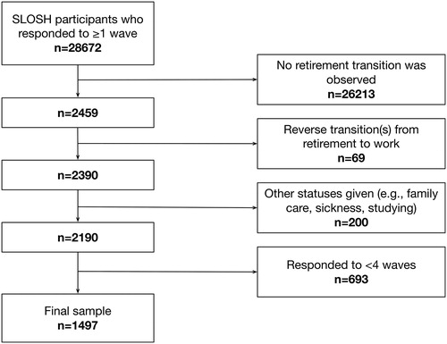
To generate the sample for the study, we first identified SLOSH participants who responded to at least one questionnaire during 2006–2016 (n = 28,672, Figure 1). Retirement was operationalized as completing the questionnaire for those in paid work at least 30% of full-time and, in the following wave, reporting being retired and completing the questionnaire for those who worked less than 30% of full-time. 22,949 participants completed at least one questionnaire for those in paid work at least 30% of full-time in 2006, 2008, 2010, 2012 and 2014, and we were able to observe a transition from paid work to retirement from one wave to the next for 2459 participants. We excluded 69 participants who reported reverse transitions from retirement to paid work (unretirement) and 200 people who reported other activities (e.g., family care), leaving 2190 eligible participants. Only participants providing ≥4 measurements were included in the analysis, generating a sample of 1497 individuals.

Figure 1. Flowchart describing selection of participants in the study.

Ascertainment of retirement and time axis

Participants were classified as retired if they described their current situation as, on a full-time basis, old age retirement or receiving another sort of pension (e.g., occupational pension). Various types of ill-health retirements (e.g., disability pension, early retirement on health grounds) were not classified as retirement, because health trajectories for these groups may vary greatly from those of other retirees (Vahtera et al., 2009; Westerlund et al., 2009).

Time was measured in the number of years before and after retirement, ranging from nine years before until nine years after retirement. The first wave at which a participant reported being retired was assigned +1. Since there is a two-year gap between waves, the pre-retirement period is −9 to −1 years, the retirement transition took place between years −1 and +1 and the post-retirement period is +3 to +9 years.

Depressive symptoms

Depressive symptoms were measured with SCL-CD₆ (Magnusson Hanson et al., 2014), a brief subscale from the (Hopkins) Symptom Checklist (SCL-90). The respondents were asked to respond on a five-category scale from 0 = not at all to 4 = extremely whether they had felt: blue, no interest in things, lethargic or low in energy, everything is an effort, they worried too much about things or blamed themselves for things. This scale has been validated and was found to have adequate construct validity, high unidimensionality and was predictive of hospitalization and antidepressant medication (Magnusson Hanson et al., 2014). The item were summed to create a 0–24 point scale. A score equal or higher to 17 was used as an indicator of major depression (Magnusson Hanson, Chungkham, Åkerstedt, & Westerlund, 2014).

Statistical methods

To identify trajectories of depressive symptoms around retirement we compared two forms of group-based trajectory modelling: the standard approach which uses polynomial link functions and a new approach using B-spline smoothers. The standard polynomial group-based trajectory model assumes that estimated trajectories follow a polynomial curve over time. Polynomial smoothing is applied to the mean of each of the k trajectories through a log-linear model. The B-spline group-based trajectory model uses a spline regression function, which is formed by connecting a set of usually cubic polynomials. In this case, k different B-spline smoothers which change over time are calculated, one for each trajectory.

For all models, depression trajectories were estimated using the censored normal model (CNORM) which is appropriate for continuous and ordinal data. For the polynomial models we used the PROC TRAJ procedure developed by Jones and Nagin (Jones, Nagin, & Roeder, 2001) for SAS software (version 9.4; SAS Institute), while for the B-spline models we used the splines library in R (R Core Team, 2014) as well as PROC TRAJ.

Once the parameters of the models were estimated, then the posterior probability of trajectory membership for each individual was estimated. Mathematical details about the models are beyond the scope of this article and can be found elsewhere (de Boor, 1978; Francis et al., 2016; Nagin, 2005).

Standard polynomial group-based trajectory models

To determine the optimal number of trajectory groups and choose the number and order of regression parameters, we followed Nagin’s two-step procedure for model selection (Nagin, 2005). First, we fitted a single trajectory model with cubic polynomial shape (third-order polynomial) for depressive symptoms. We then augmented the number of trajectories from a single to a two-trajectory model where both trajectories were cubic. This procedure to augment the number of trajectories was repeated until there was no longer evidence for improvement in model fit. At a second step, we selected the shape of the trajectories (cubic, quadratic, linear) for the selected model in step 1 by evaluating the statistical significance of the cubic terms. If cubic components were not significant, we tested models with quadratic and linear trajectories. Linear components were always retained irrespective of statistical significance (Louvet, Gaudreau, Menaut, Genty, & Deneuve, 2009).

B-spline group-based trajectory models

The B-spline trajectories were obtained according to the procedure suggested in Francis et al.: we first calculated the cubic B-spline basis for the time variable with 1 to 5 knots (the points where the polynomial segments connect), using the bs() function in the R library splines. Next we used the PROC TRAJ procedure in order to fit the B-spline group-based trajectory models where we included the B-splines as time-varying covariates, setting the polynomial order to zero (Francis et al., 2016). We fitted a sequence of models with one to eight trajectory groups and one to five knots (the points where the polynomial segments connect). The number of knots represented the degree of smoothing with higher number of knots resulting in more local polynomials and greater ability to follow the underlying data. In order to choose the location and number of knots we examined the information criteria described in the following section.

Test statistics for model selection

The Bayesian Information Criterion (Schwarz, 1978) and the Integrated-Complete Likelihood BIC criterion (ICL_BIC) (McLachlan & Peel, 2004) were used to determine the best model fit. The selection of the model with the largest value is recommended (Nagin, 2005). In order to compare two models with different numbers of groups an approximation of the Bayes factor was used, where evidence for the more complex model is a value larger than five (Andruff, Carraro, Thompson, Gaudreau, & Louvet, 2009; Jones & Nagin, 2007; Jones et al., 2001). Model adequacy was tested using the average posterior probabilities (APP) of group membership, which measure the likelihood for each individual to belong to its assigned group (preferable >0.7) (Nagin, 2005). We also assessed whether the models distinguished distinctive features of the data in a parsimonious way by visual inspection of the trajectories. Finally, R² values were reported as a measure of goodness of fit.

Results

Observed individual trajectories of depressive symptoms

Among the 1497 included participants in the analysis, four measurements were available for 537 (35.9%), five measurements were available for 717 (47.9%) while six measurements were available for 243 (16.2%) individuals. The respondents’ age range varied from 46 to 77 years old, while the majority were women (54.5% in 2006) compared to men (45.5% in 2006).

There was considerable variation in depressive symptoms around retirement. The median depressive symptoms scores (and interquartile ranges) were: t= −9 years: 4 (2 to 9), t= −7: 4 (1 to 8), t= −5: 3 (1 to 7), t= −3: 3 (1 to 7), t= −1: 3 (1 to 7), t = 1: 2 (0 to 4), t = 3: 2 (0 to 4), t = 5: 1 (0 to 5), t = 7: 2 (0 to 5) and t = 9: 3 (0 to 6) for the ten time points around old age retirement. Only 7.7% of the participants had no more than a one-point difference between the highest and lowest depressive symptoms scores. A depressive score ≥17 at least once during follow-up was reported by 7.6% of the participants.

Polynomial trajectory models of depressive symptoms around old age retirement

All the statistical fit indices indicated the seven-group model was superior to the other models (Table 1). However, both the APP values and the entropy deteriorated for this model compared to the six-group model. Thus we concluded that the six-group model was more appropriate than the seven-group solution. The six-group model was then refined until the highest polynomial coefficient for each trajectory group was statistically significant from zero. The final model was therefore a six-group model where three groups had a cubic, two groups had a quadratic and one group had a linear order. Figure 2a shows the estimated trajectories of depressive symptoms (solid lines), the observed mean depressive symptoms (dashed lines) around retirement for the six-group solution and group sizes. Five broadly horizontal groups (groups 1 to 5) were distinguished by severity of depressive symptoms (very low, low, middling, moderate high, high) and the additional group (Group 6) reported high levels of depressive symptoms 5–7 years before retirement which decreased to a low level over the period of follow-up.

Figure 2. (a) Estimated and observed means of depressive symptoms around retirement from the polynomial group-based trajectory model with six groups described by three cubic, two quadratic and one linear polynomial. Swedish Longitudinal Occupational Survey of Health 2006–2016, n = 1497. (b) Estimated and observed means of depressive symptoms around retirement from the B-spline group-based trajectory model with six groups and five knots. Swedish Longitudinal Occupational Survey of Health, 2006–2016, n = 1497.

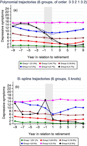
Table 1. Fit indices (BIC, ICL-BIC values) and the log-Bayes factor from (a) polynomial models with 1 to 8 groups and cubic order as well as polynomial model with 6 groups and selected shapes (b) B-spline models with 1–8 groups and 1–5 knots. Swedish Longitudinal Occupational Survey of Health, 2006–2016, n = 1497.

	Polynomial	Model
Number of groups	Polynomial order	BIC	Bayes factor	ICL-BIC	Bayes factor
1	3	−19633.8		−19631.8	–
2	3 3	−18627.5	2012.6	−18626.6	−18600.9
3	3 3 3	−18313.6	627.7	−18312.7	−18273.8
4	3 3 3 3	−18196.1	235.0	−18195.2	−18143.0
5	3 3 3 3 3	−18158.6	75.1	−18157.7	−18092.2
6	3 3 3 3 3 3	−18152.5	12.2	−18151.6	−18072.8
7	3 3 3 3 3 3 3	−18146.0	12.9	−18145.2	−18053.1
8	3 3 3 3 3 3 3 3	−18151.9	−11.7	−18151.0	−18045.7
6	3 3 2 3 2 1	−18140.9	23.2^a	−18140.0	27.2^a
	B-spline model
Number of groups	1 knot	2 knots	3 knots	4 knots	5 knots	Bayes factor
BIC
1	−19760.5	−19699.8	−19656.7	−19637.7	−19628.6	–
2	−18788.4	−18706.1	−18665.7	−18639.2	−18625.6	2005.8
3	−18472.3	−18381.3	−18347.9	−18320.8	−18316.2	618.7
4	−18380.0	−18282.5	−18248.8	−18220.4	−18213.9	204.8
5	−18377.5	−18277.0	−18240.9	−18212.8	−18213.8	0.1
6	−18356.9	−18296.2	−18245.1	−18176.5	−18176.4	74. 8
7	−18372.7	−18242.9	−18225.9	−18175.9	−18193.3	−33.9
8	−18370.1	−18216.2	−18203.4	−18156.9	−18221.6	−56.6
ICL–BIC
1	−19758.4	−19697.8	−19654.7	−19635.7	−19628.5	–
2	−18787.5	−18705.2	−18664.7	−18638.3	−18624.6	2007.6
3	−18471.4	−18380.4	−18347.0	−18320.0	−18315.3	618.6
4	−18379.1	−18281.6	−18247.9	−18219.5	−18212.9	204.8
5	−18376.7	−18276.1	−18240.0	−18211.9	−18212.9	0.0
6	−18356.0	−18295.4	−18244.2	−18175.6	−18175.5	74.8
7	−18372.0	−18242.1	−18225.0	−18175.0	−18192.4	−33.9
8	−18369.2	−18215.3	−18202.6	−18156.0	−18220.7	−56.6

^a The last model is compared to the six-group (3 3 3 3 3 3) model.

Model adequacy and fit were assessed using the APP and R² values (Results not shown). For all trajectory groups the APP were close to or higher than the recommended value of 0.7. This was an indication that the model assigned individuals to different groups with little ambiguity. R² values indicated satisfactory fit for most groups. Examination of Figure 2a indicated that estimates of polynomial trajectories showed uplifts at both ends of the time axis which were unsupported by observed mean depressive symptoms.

B-spline trajectory models of depressive symptoms around old age retirement

All the statistical fit indices indicated the model with six groups and five knots as superior to the other models (Table 1). Figure 2b shows the estimated trajectories of depressive symptoms (solid lines), the observed mean depressive symptoms (dashed lines) around retirement for the six-group solution and the group sizes. Most (85.9%) individuals were classified into groups 1, 2 or group 3. The proportion of individuals in the other groups varied from 2.8% to 8.5%.

Four broadly horizontal groups (groups 1 to 3 and 5) were distinguished by severity of depressive symptoms (very low, low, middling, high). One group (Group 4, 8.5%) reported high levels of depressive symptoms 5–7 years before retirement which decreased to a medium level over the period of retirement and increasing levels of depressive symptoms after retirement. The last group (group 6, 2.8%) was characterized by increasing level of depressive symptoms leading up to retirement, a slight decline around retirement and further decreases following retirement.

Model adequacy and fit were assessed using the APP and R² values (Results not shown). For all trajectory groups, the APP were close or higher to the recommended value of 0.7. This was an indication that the model assigned individuals to different groups with little ambiguity. R² values indicated very good fit for all the groups.

Comparison of polynomial and B-spline trajectories

Both polynomial and B-spline group-based trajectory models resulted in a six-group solution, in which the various groups were broadly similarly sized across the two methods. APP values ranged above the recommended value of 0.7 for both models although they were a little higher for the B-spline model in four of the six groups compared to the polynomial model. Both R² values and visual examination of the figures indicated that the B-spline model fitted the observed data better than the polynomial model. The polynomial model did not capture the fluctuations in observed data in most groups (which could be related to the order of polynomial selected). It also produced unexpected changes in direction of the curves, which were not supported by the data, and which could encourage misleading conclusions to be drawn. In contrast, the B-spline model provided a closer fit to the observed data, captured the fluctuations of the data and did not generate uplifts which did not exist in the data.

The shapes of trajectories were broadly similar for four of the six trajectories in terms of severity and stability (groups 1, 2, 3 and 5) but differed for groups 4 and group 6. For group 4, the B-spline model suggested a steep decrease from high to medium level during retirement while the polynomial model suggested a more flattened shape. Although the observed mean number of depressive symptoms look broadly similar for both models, the B-spline model reproduced the shape of the trajectories more precisely than the polynomial model. For group 6, the models resulted in trajectories that differed in the pattern of observed mean depressive symptoms. Investigation of randomly selected observed individuals for this group indicated that the polynomial model grouped together individuals with more heterogeneous behavior compared to the B-spline model. As a result, the average depression for the B-spline model seemed more representative of the behavior of the individuals in the group compared to the polynomial model.

In order to have a better understanding of the two methods, we examined the trajectories obtained when starting from one group and then gradually increasing the number of groups until the optimal model with six groups (Supplementary Figure 1). The B-spline and polynomial trajectories were broadly similar from one to four groups but differed when having more than four groups. The B-splines reproduced the shape of trajectories more precisely in all cases than the polynomial model, which usually produced more flattened trajectories and failed to capture distinctive features of the observed data, such as abrupt changes in trajectory which could occur at the retirement transition, years –1 to +1. The groups created by the two methods were highly homogeneous from two to four groups but the degree of heterogeneity increased as additional groups were added (Results not shown). Overall, compared to polynomials, B-spline trajectories better represented the complex dynamic shapes of depressive symptoms in relation to retirement.

Discussion

In the current study, we examined variations in the course of depressive symptoms over time in relation to retirement using group-based trajectory modelling. Our findings support the argument that individuals vary in their responses to retirement (Pinquart & Schindler, 2007; Wang, 2007), highlighting the need to examine the course of individual psychological health in a way that allows demarcation of groups with diverging symptoms trajectories (Henning et al., 2016; Lindwall et al., 2017) and using a method that is sufficiently flexible to model complex variations such as short-term cyclical patterns.

This study, for the first time, uses health data to compare two approaches to estimating the models: the standard approach using a polynomial function of time and a new approach employing B-splines to model the shape of trajectories over time. Estimation with B-splines presented a number of advantages: greater homogeneity within the groups, avoidance of spurious uplifts, and the capacity to model abrupt shifts in trajectories taking place at retirement. The advantages of fitting B-splines have previously been presented with an application to criminology data (Francis et al., 2016); we confirm and extend the applicability of this statistically robust method to symptoms-based mental health trajectories in relation to a common life event.

There are a number of important implications of this work for clinical and epidemiological research into depression. Methods that provide for lag or cumulative effects usually neglect individual differences in the transition to retirement and do not capture the implicit heterogeneity of such data. Traditional approaches such as hierarchical and latent curve modelling may be unsuitable for modelling non-monotonic trajectories (trajectories that both increase and decrease), and may consequently provide undue evidence of stability in the course of depressive symptoms which is an artefact due to the fact that the different trajectories may offset one another. Group-based trajectory modelling uses polynomial functions which are adapted to long-term developments rather than sudden changes. Estimating trajectories with B-splines extends group-based trajectory modelling to the study of changes that are highly dynamic and not polynomial shaped, in particular to abrupt changes such as those that may occur in relation to life events. This is important since life events such as onset of physical illness, job loss and relationship breakdown are common triggers of episodes of major depressive disorder. The effects of life events, which may differ among sub-groups differentiated by unobserved variables, can now be studied with B-spline group-based trajectory models.

The locality of B-spline estimation approaches avoids the generation of patterns unsupported by the data, such as artefactual uplifts, which may be erroneously interpreted as late improvements or declines. Consequently, this method provides better understanding of the dynamics of symptoms-based data over time. More accurate longitudinal modelling of such data will support analyses of the causes, risk factors and consequences of temporal changes in the course of illness such as major depressive disorder. Future research using B-spline group-based trajectory modelling may improve understanding of the role of life events, in particular the characteristics of sub-groups that are particularly vulnerable and resilient, providing insight into potentially modifiable vulnerability and protective factors. Such knowledge may assist with identification of groups which might benefit from therapeutic interventions and can be used to help plan prevention and treatment strategies.

Strengths and limitations

In addition to the more flexible modelling of trajectories offered by the use of B-splines, strengths of this study included its large sample, which is approximately representative of the Swedish working population. The longitudinal design contained participants contributing at least four measurements across six waves which is above the minimum required to estimate cubic models. Another advantage of the methods used is that they can handle missing data in the dependent variables by assuming that missing data on dependent variables are missing at random and by using all available observations on the dependent measure. Both methods of estimating group-based trajectories resulted in similar observed mean depressive symptoms, at least for the main groups, which gave support for the robustness of the findings.

One limitation from a technical point of view is that it is currently more time-consuming to calculate estimates with B-splines rather than polynomials, since an automatic procedure is lacking, although there are possibilities to use several software packages to obtain results. In addition, the B-spline model required double the number of parameters to be estimated compared to the polynomial model. Another possible limitation is that the generalizability of these results may be limited due to selective dropout (a higher proportion of responders than non-responders to SLOSH are women, older, born in Sweden, married, have a university education and work in the government sector). A particular issue is that people with ill-health retirements were not included in the study which, while reducing the risk that the observed patterns are due to retirement resulting from the development of depressive symptoms rather than vice versa, means that the results do not necessarily apply to retirement due to ill health. While it would be interesting to examine trajectories of people with ill-health retirements in separate analyses, lack of power prevented us from performing these analyses here. Lastly, exposure to poorer finances in retirement may affect assignment to trajectory groups, but it was not possible to consider differentially subjects according to their level of pension due to lack of pension income data.

Future work

There are a number of ways that investigators can apply and extend this new method of group-based trajectory modelling with B-splines, including to other sorts of data, e.g., biomarker data; other types of life events; and in relation to interventions. Application of the method in other contexts would clarify the broader possibilities offered by this approach.

Since the aim of this study was not to examine the effects of individual-level characteristics, although certain covariates (age, sex, chronic illness, socio-economic level, education and income) were significantly associated with some of the trajectories, these results are not presented here. Group-based trajectory modelling with B-splines can be used in future work to study the effect of multiple variables on changes in level of depressive symptoms at the retirement transition (Lindwall et al., 2017). Although it would also be useful from a public health perspective to report results relating major depressive symptoms (e.g., scores equal to or higher than a cut-off of 17), we did not do so due to convergence problems.

In our analyses, we followed the conventional two-stage process in which an unconditional mixture model (i.e., without covariates) was first fitted to determine the number of distinct trajectory groups, and subject-specific characteristics were considered once the clusters were identified. This type of analysis allows for characteristics to be identified that predict the developmental course of a behavior (Nagin, 2005). However, it is possible to condense this process into one step, by including the covariates in the model (conditional mixture model), i.e., adding covariates, beyond time, to the trajectories themselves (Huang, Brecht, Hara, & Hser, 2010; Schiltz, 2015). This approach allows for the possibility that life events may cause individuals to change trajectory groups (Nagin, 2005). The introduction of covariates into the specification of the trajectory has implications for the number and shape of groups, and interpretation of the parameters (Nagin, 2005). These differences may be due to the associations of trajectories with the covariates and the distribution of covariates, implying effect modification. Future work is likely to clarify under which circumstances estimation of unconditional or conditional mixture models is more suitable (Huang et al., 2010; Muthén, 2003; Nagin, 2005).

From a statistical methods perspective, future work could extend B-spline group-based trajectory modelling not only for descriptive purposes but also for performing within-trajectory group causal inference with observational longitudinal data or for achieving balance in propensity score-based causal inference (Haviland & Nagin, 2005, 2007). An additional extension would be the use of B-splines in the estimation of multi-trajectory models, which allow for complex characterizations of developmental history typologies and identification of latent strata in the data.

Conclusion

In estimating group-based trajectory models, we recommend that investigators consider use of B-splines as an alternative to the polynomial link function, since this method enables more flexible and accurate modelling of abrupt changes and other trajectories with complex shapes. Improved modelling of symptoms-based trajectories will support advances in research into vulnerability factors and interventions, which may ultimately reduce the burden of disease.

Disclosure statement

No potential conflict of interest was reported by the authors.

References

- Amick, B. C., McLeod, C. B., & Bültmann, U. (2016). Labor markets and health: an integrated life course perspective. Scandinavian Journal of Work, Environment & Health, 42(4), 346–353. doi:10.5271/sjweh.3567
- Andreescu, C., Chang, C.-C. H., Mulsant, B. H., & Ganguli, M. (2008). Twelve-year depressive symptom trajectories and their predictors in a community sample of older adults. International Psychogeriatrics, 20(2), 221–236. doi:10.1017/S1041610207006667
- Andruff, H., Carraro, N., Thompson, A., Gaudreau, P., & Louvet, B. (2009). Latent class growth modelling: A tutorial. Tutorials in Quantitative Methods for Psychology, 5(1), 11–24. doi:10.20982/tqmp.05.1.p011
- Blazer, D. G. (2003). Depression in late life: Review and commentary. The Journals of Gerontology. Series A, Biological Sciences and Medical Sciences, 58(3), 249–265.
- Bogner, H. R., Morales, K. H., Reynolds, C. F., Cary, M. S., & Bruce, M. L. (2012). Course of depression and mortality among older primary care patients. The American Journal of Geriatric Psychiatry: Official Journal of the American Association for Geriatric Psychiatry, 20(10), 895–903. doi:10.1097/JGP.0b013e3182331104
- Colman, I., & Ataullahjan, A. (2010). Life course perspectives on the epidemiology of depression. Canadian Journal of Psychiatry. Revue Canadienne De Psychiatrie, 55(10), 622–632. doi:10.1177/070674371005501002
- de Boor, C. (1978). A Practical Guide to Spline. Volume27. New York: Springer. doi:10.2307/2006241
- Francis, B., Elliott, A., & Weldon, M. (2016). Smoothing group-based trajectory models through B-splines. Journal of Developmental and Life-Course Criminology, 2(1), 113–133. doi:10.1007/s40865-016-0025-6
- Goldstein, H. (2010). Multilevel Statistical Models (4th ed.). Chichester, West Sussex: Wiley.
- Haviland, A. M., & Nagin, D. S. (2005). Causal inferences with group based trajectory models. Psychometrika, 70(3), 557–578. doi:10.1007/s11336-004-1261-y
- Haviland, A. M., & Nagin, D. S. (2007). Using group-based trajectory modeling in conjunction with propensity scores to improve balance. Journal of Experimental Criminology, 3(1), 65–82. doi:10.1007/s11292-007-9023-3
- Heikkinen, E. (2011). A life course approach: Research orientations and future challenges. European Review of Aging and Physical Activity, 8(1), 7–12. doi:10.1007/s11556-010-0069-2
- Henning, G., Lindwall, M., & Johansson, B. (2016). Continuity in well-being in the transition to retirement. GeroPsych, 29(4), 225–237. doi:10.1024/1662-9647/a000155
- Huang, D., Brecht, M.-L., Hara, M., & Hser, Y.-I. (2010). Influences of a covariate on growth mixture modeling. Journal of Drug Issues, 40(1), 173–194.
- Jokela, M., Ferrie, J. E., Gimeno, D., Chandola, T., Shipley, M. J., Head, J., … Kivimäki, M. (2010). From midlife to early old age: Health trajectories associated with retirement. Epidemiology, 21(3), 284–290. doi:10.1097/EDE.0b013e3181d61f53
- Jones, B. L., & Nagin, D. S. (2007). Advances in group-based trajectory modeling and an SAS procedure for estimating them. Sociological Methods & Research, 35(4), 542–571. doi:10.1177/0049124106292364
- Jones, B. L., Nagin, D. S., & Roeder, K. (2001). A SAS procedure based on mixture models for estimating developmental trajectories. Sociological Methods & Research, 29(3), 374–393. doi:10.1177/0049124101029003005
- Kwon, E., Kim, B., Lee, H., & Park, S. (2017). Heterogeneous trajectories of depressive symptoms in late middle age: Critical period, accumulation, and social mobility life course perspectives. Journal of Aging and Health. doi:10.1177/0898264317704540
- Leinonen, T., Lahelma, E., & Martikainen, P. (2013). Trajectories of antidepressant medication before and after retirement: The contribution of socio-demographic factors. European Journal of Epidemiology, 28(5), 417–426. doi:10.1007/s10654-013-9792-0
- Linda L Magnusson Hanson, Constanze Leineweber, Viktor Persson, Martin Hyde, Töres, Theorell, & Hugo, Westerlund. (2018). Cohort Profile: The Swedish Longitudinal Occupational Survey of Health (SLOSH). International Journal of Epidemiology, 47(3):691–692i. doi:10.1093/ije/dyx260.
- Lindwall, M., Berg, A. I., Bjälkebring, P., Buratti, S., Hansson, I., Hassing, L., … Johansson, B. (2017). Psychological health in the retirement transition: Rationale and first findings in the Health, Ageing and Retirement Transitions in Sweden (HEARTS) Study. Frontiers in Psychology, 8, 1634. doi:10.3389/fpsyg.2017.01634
- Louvet, B., Gaudreau, P., Menaut, A., Genty, J., & Deneuve, P. (2009). Revisiting the changing and stable properties of coping utilization using latent class growth analysis: A longitudinal investigation with soccer referees. Psychology of Sport and Exercise, 10(1), 124–135. doi:10.1016/j.psychsport.2008.02.002
- Magnusson Hanson, L. L., Chungkham, H. S., Åkerstedt, T., & Westerlund, H. (2014). The role of sleep disturbances in the longitudinal relationship between psychosocial working conditions, measured by work demands and support, and depression. Sleep, 37(12), 1977–1985. doi:10.5665/sleep.4254
- Magnusson Hanson, L. L., Westerlund, H., Leineweber, C., Rugulies, R., Osika, W., Theorell, T., & Bech, P. (2014). The Symptom Checklist-core depression (SCL-CD6) scale: Psychometric properties of a brief six item scale for the assessment of depression. Scandinavian Journal of Public Health, 42(1), 82–88. doi:10.1177/1403494813500591
- McLachlan, G., & Peel, D. (2004). Finite Mixture Models. New York: John Wiley & Sons.
- Modrego, P. J., & Ferrández, J. (2004). Depression in patients with mild cognitive impairment increases the risk of developing dementia of Alzheimer type: A prospective cohort study. Archives of Neurology, 61(8), 1290–1293. doi:10.1001/archneur.61.8.1290
- Musliner, K. L., Munk-Olsen, T., Eaton, W. W., & Zandi, P. P. (2016). Heterogeneity in long-term trajectories of depressive symptoms: Patterns, predictors and outcomes. Journal of Affective Disorders, 192(Supplement C), 199–211. doi:10.1016/j.jad.2015.12.030
- Muthén, B. (1989). Latent variable modeling in heterogeneous populations. Psychometrika, 54(4), 557–585. doi:10.1007/BF02296397
- Muthén, B. (2003). Statistical and substantive checking in growth mixture modeling: Comment on Bauer and Curran (2003). Psychological Methods, 8(3), 369–377; discussion 384–393. doi:10.1037/1082-989X.8.3.369
- Nagin, D. S. (1999). Analyzing developmental trajectories: A semiparametric, group-based approach. Psychological Methods, 4(2), 139–157. doi:10.1037/1082-989X.4.2.139
- Nagin, D. S. (2005). Group-Based Modeling of Development. Cambridge, MA: Harvard University Press.
- Nagin, D. S., & Odgers, C. L. (2010). Group-based trajectory modeling in clinical research. Annual Review of Clinical Psychology, 6, 109–138. doi:10.1146/annurev.clinpsy.121208.131413.
- Oksanen, T., Vahtera, J., Westerlund, H., Pentti, J., Sjösten, N., Virtanen, M., … Kivimäki, M. (2011). Is retirement beneficial for mental health? Antidepressant use before and after retirement. Epidemiology, 22(4), 553–559. doi:10.1097/EDE.0b013e31821c41bd
- Peristera, P., Westerlund, H., Magnusson Hanson L. L. (2018). Paid and unpaid working hours among Swedish men and women in relation to depressive symptom trajectories: results from four waves of the Swedish Longitudial Occupational Survey of Health. BMJ Open, 8(6):e017525. doi:10.1136/bmjopen-2017-017525.
- Pinquart, M., & Schindler, I. (2007). Changes of life satisfaction in the transition to retirement: a latent-class approach. Psychology and Aging, 22(3), 442–455. doi:10.1037/0882-7974.22.3.442
- R Core Team. (2014). R: A language and environment for statistical computing, Vienna, Austria. Retrieved from October 26, 2017 http://www.R-project.org/.
- Raudenbush, S. W., & Bryk, A. S. (2001). Hierarchical Linear Models: Applications and Data Analysis Methods (2nd ed.). Thousand Oaks, CA: SAGE Publications, Inc.
- Schiltz, J. (2015). A generalization of Nagin’s finite mixture model. Retrieved from http://orbilu.uni.lu/handle/10993/18384.
- Schwarz, G. (1978). Estimating the dimension of a model. The Annals of Statistics, 6(2), 461–464.
- Vahtera, J., Westerlund, H., Hall, M., Sjösten, N., Kivimäki, M., SalO, P., … Zins, M. (2009). Effect of retirement on sleep disturbances: The GAZEL prospective cohort study. Sleep, 32(11), 1459–1466.
- Vos, T., Abajobir, A. A., Abate, K. H., Abbafati, C., Abbas, K. M., Abd-Allah, F., … Murray, C. J. L. (2017). Global, regional, and national incidence, prevalence, and years lived with disability for 328 diseases and injuries for 195 countries, 1990–2016: A systematic analysis for the Global Burden of Disease Study 2016. The Lancet, 390(10100), 1211–1259.
- Wang, M. (2007). Profiling retirees in the retirement transition and adjustment process: Examining the longitudinal change patterns of retirees’ psychological well-being. The Journal of Applied Psychology, 92(2), 455–474. doi:10.1037/0021-9010.92.2.455
- Westerlund, H., Kivimäki, M., Singh-Manoux, A., Melchior, M., Ferrie, J. E., Pentti, J., … Vahtera, J. (2009). Self-rated health before and after retirement in France (GAZEL): A cohort study. The Lancet, 374(9705), 1889–1896. doi:10.1016/S0140-6736(09)61570-1
- Westerlund, H., Vahtera, J., Ferrie, J. E., Singh-Manoux, A., Pentti, J., Melchior, M., … Kivimäki, M. (2010). Effect of retirement on major chronic conditions and fatigue: French GAZEL occupational cohort study. BMJ, 341, c6149.
- Zins, M., Guéguen, A., Kivimaki, M., Singh-Manoux, A., Leclerc, A., Vahtera, J., … Goldberg, M. (2011). Effect of retirement on alcohol consumption: Longitudinal evidence from the French Gazel Cohort Study. PLOS ONE, 6(10), e26531.