In situ strain investigation during laser welding using digital image correlation and finite-element-based numerical simulation

ABSTRACT

In situ strain evolution during laser welding has been measured by means of digital image correlation to assess the susceptibility of an advanced high strength automotive steel to solidification cracking. A novel method realised using auxiliary illumination and optical narrow bandpass filter allowed strain measurements as close as 1.5 mm from the fusion boundary with good spatial and temporal resolution. A finite-element thermomechanical model of the welding process supports the experimentally measured transverse strain. The validated finite-element numerical model can be used to assess the local strain and associated stress conditions which influences weldability and in particular, solidification cracking.

Keywords:

• In situ strain
• laser welding
• digital image correlation
• FEM
• weld defects

Introduction

In the last decades, laser beam welding has become increasingly popular in the automotive industry. The high power density ( W m⁻²) facilitates the welding of steels at high speed, thereby increasing productivity. During welding, materials experience non-uniform heating and cooling cycles; this results in the development of stresses, deformation and distortion. Apart from metallurgical effects, the evolution of strains and stresses in the weld and heat-affected zone determines the weldability of an alloy. An important indicator of weldability is its resistance to cracking, either in the weld or in the heat-affected zone. One of the major defects encountered in the casting and welding industries is hot tearing, also referred to as solidification cracking [1,2]. Accurate determination of local strain and associated stresses produced during welding is important to generate a better understanding of welding-induced deformation and defect formation, including solidification cracking.

One of the methods to measure full-field displacement and strain during a thermomechanical process is digital image correlation (DIC). With this technique, camera(s) acquire digital images of a random speckle pattern on a specimen during the deformation process. To correlate the reference image and the deformed image, an image is divided into subsets of pixels. These subsets are tracked to obtain displacement in the horizontal and vertical directions [3]. The DIC technique has been used to measure strains at grain level [4], study failure in thermal barrier coatings [5], investigate fatigue cracks [6], etc. DIC is generally applied ex situ for welding-related measurements. In situ studies are hindered by the intense light emitted during welding, which renders observation close to the fusion boundary difficult. There are only a few reported studies in which the in situ strains are measured during welding [7–10]. In these studies, displacement fields were measured either far from the weld centreline or on the underside of the specimen to minimise the effect of intense light and heat.

In this work, the DIC technique is applied on the upper surface close to a weld to measure in situ transverse strain fields during laser welding of a commercial advanced high strength automotive steel (AHSS).

Experimental set-up

Bead-on-plate welding experiments were performed using a 3 kW Nd:YAG laser in the keyhole mode. A laser power of 1100 W and a welding speed of 10 mm s⁻¹ were used in all the experiments. Rectangular transformation induced plasticity (TRIP) steel sheets of dimensions  mm² and 1.25 mm thickness were welded. The chemical composition of the steel is C – 0.19, Mn – 1.63, Al – 1.1 and Si – 0.35 (all in weight %). The experimental arrangement used in this work is shown schematically in Figure 1(a). This figure includes the coordinate system used for DIC measurements. The starting beam position was at x=0 mm, y=13 mm and t=0 s. The distance of the laser beam from the free edge was maintained at 13 mm. Similar bead-on-plate experiments are conducted as standard tests to determine the hot cracking susceptibility of steels used in the automotive sector [12]. Random speckle patterns were applied on the top surface using a high-temperature commercial paint. The paint can withstand temperature up to . The temperature during the welding process was measured at several positions close to the fusion boundary by spot-welded K-type thermocouples. A full penetration weld bead with a width of 2.8 mm was obtained.

Figure 1. (a) Schematic of the laser bead-on-plate welding and DIC measurement set-up, (b) Typical emission spectra of an Nd:YAG laser plume on an iron-based specimen. The graph is replotted from [11]. The position of the optical narrow bandpass filter in this spectrum is also indicated, (c) Simulated and experimental temperature cycle. Here, T(1) refers to the measured temperature cycle at a distance of 3 mm from the weld centreline towards the free edge. T(2) and T(3) are the measured temperature cycles at a distance of 2.5 and 4 mm from the weld centreline towards the constrained edge.

A LIMESS Q-400-3D DIC system [13] along with a commercial software package Istra 4D was used to capture and analyse images at a frame rate of 8 Hz. Before carrying out image correlation on the specimen surface, calibration of the DIC cameras was carried out using 10 images of a translated and rotated planar dot pattern of known spacing. A typical emission spectra of the laser plume on an iron-based specimen are shown in Figure 1(b) [11]. To minimise the effect of intensity of laser plume light, two auxiliary high intensity 30 W LEDs with a wavelength of 450 nm were used to illuminate the top surface of the specimen. Corresponding optical narrow bandpass filters with a centre wavelength of 450 nm and a full-width half maxima (FWHM) of 10 nm were placed in front of the lenses to minimise the effect of plume light. This approach allowed measurement of displacement fields as close as 1.5–2 mm from the fusion boundary.

Modelling approach

A finite-element (FE)-based thermal elasto-plastic model of the welding process was developed to complement the understanding of experimental results. After validation, the FE-model can be used to ascertain strain fields in regions where laboratory experimental measurements are impractical. A sequentially coupled 3D FE thermal elasto-plastic model with isotropic hardening was developed to numerically calculate the temperature and the strain fields for the laser bead-on-plate welding process. In the first step, a heat transfer analysis was conducted to retrieve the time-dependent temperature field.

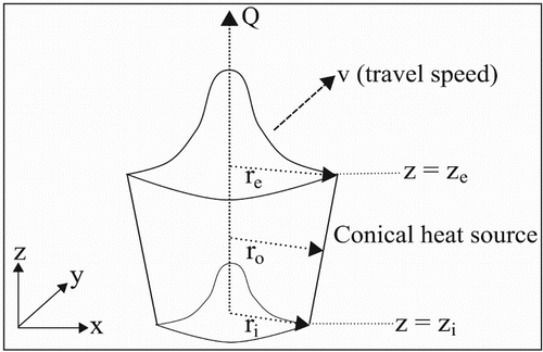
A 3D conical heat source with Gaussian distribution, as shown in Figure 2, was adapted to describe the laser beam heat input [14,15]. The power density distribution at any plane perpendicular to the z-axis may be expressed as (1a) with (1b) and (1c) where is the total volumetric heat flux in W m⁻³, is the maximum heat source intensity in W m⁻³, r is the radial coordinate of interior point, and are the top and bottom radius of the conical heat source, respectively. and are the z coordinates of the top and bottom surfaces, respectively. The height of the cone, i.e. was assumed to be the thickness of the steel sheet and , were adjusted to obtain the weld dimensions observed experimentally.

Figure 2. Schematic of the 3D Gaussian conical heat source used in this work.

Subsequently, the temperature field history was applied as a thermal load for simulating the thermomechanical response of the material. This kind of sequential coupling approach is common in welding research [16–20]. Commercial software, COMSOL was used for this purpose. Quadratic elements with a minimum mesh size of  mm² and depth 1 mm were used.

The thermophysical and mechanical properties of the TRIP steel used in this model were taken from [21], based on a steel with a similar chemical composition. Latent heat during the solid-to-liquid (and vice versa) phase transformation is included in the temperature-dependent-specific heat capacity of the material. The release of latent heat during solidification is based on the phase fraction obtained using the Scheil–Gulliver solidification approximation. The thermal expansion coefficient (α) in the two phase region is also assumed to be dependent on the phase fractions. Thermo-Calc was used to obtain the temperature-dependent phase fraction data based on the chemical composition of the steel.

In the mechanical analysis, the translational and rotational displacements at the fixed edges of the sheet were constrained. The out-of-plane movement on the surfaces in contact with the clamp was also set to zero.

Results and discussion

Figure 1(c) shows the measured and simulated thermal cycle at thermocouple locations T(1), T(2) and T(3), respectively. T(1) refers to the measured temperature cycle at a distance of 3 mm from the weld centreline towards the free edge. T(2) and T(3) are the measured temperature cycles at a distance of 2.5 and 4 mm from the weld centreline towards the constrained edge. Good agreement was found between the experimental and simulated thermal cycles. Therefore, time–temperature profiles in the heat transfer model were subsequently imported to the thermomechanical model and the thermomechanical response of the material was simulated.

Figure 3(a) shows the spatial distribution of transverse strain (in %) at t=3.0 s on a surface 2 mm from the fusion boundary. The top image shows the numerically computed distribution. The bottom image overlaying the speckle pattern shows the experimentally measured distribution. At some locations, black spots are seen in the strain map. The measurement could not be performed at these locations due to data distortion caused by fume and spatter.

Figure 3. (a) Spatial distribution of transverse strain (in %) at t=3.0 s. Top image shows the distribution calculated using the FE-based model. The bottom image overlaying the speckle pattern shows the strain distribution measured using the DIC technique. The coordinate system used is the same as that used in Figure 1(a), (b) experimentally measured and numerically computed spatial distribution of transverse strain (in %) along the line H1 and H2 at t=1.75 s, (c) experimentally measured and numerically computed spatial distribution of transverse strain (in %) along the line H1 and H2 at t= 2.25 s, (d) experimentally measured and numerically computed temporal distribution of transverse strain (in %) at P1, (e) experimentally measured and numerically computed temporal distribution of transverse strain (in %) at P2, (f) experimentally measured and numerically computed temporal distribution of transverse strain (in %) at P3.

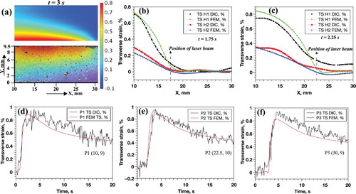
The transverse strain (TS) field during welding was measured at t=1.75 s and t=2.25 s along lines H1 and H2 parallel to the weld (Figure 1(a)) of length 20 mm and at a distance of 2 mm and 5.5 mm from the fusion boundary, respectively. The starting coordinates of lines H1, H2 are (10, 9.5) mm and (10, 6) mm, respectively. Temporal evolution of transverse strain was measured at points P1  mm P2  mm and P3  mm. The coordinates of the points are mentioned in the brackets. Transverse strain data at these locations were also extracted from the FE-based numerical study.

Figure 3(b,c) show both the experimentally measured and numerically computed distribution of transverse strain (in %) along lines H1 and H2 at t=1.75 s and t=2.25 s. The strain distribution measured by the DIC technique is comparable with the numerical results. Owing to the optical filtering of the intense laser plume light, a good spatial resolution close to the fusion boundary is achieved. Deviation of the numerically obtained transverse strain distribution along line H1 at t=2.25 s compared to the experimental results could be due to the underestimated thermal conductivity. At t=1.75 s, the laser beam is at a distance of 7.5 mm from the starting points of lines H1 and H2. At this time, the measured transverse strain decreases at a rate of  mm along the line H1, while it decreases at a rate of  mm along the line H2. At a distance of ≈2.5 mm in front of the laser beam, the transverse strain approaches zero. As the laser beam progresses further into the specimen, the transverse strain gradient along H1 and H2 direction decreases.

Figure 3(d–f) shows the measured and computed temporal transverse strain evolution at points P1, P2 and P3, respectively. The strain reaches a peak value when the laser beam approaches these positions. There is reasonable agreement between the experimental and numerical results. Numerically calculated peak transverse strain in the case of P3 was 0.0083, while the measured peak strain was 0.0093. Compared to P2 and P3, a large noise in transverse strain was observed at P1. This could be due to the loss of DIC data integrity in close proximity of P1 during welding. Error in displacement measurement of a subset occurs when comparing images with insufficient viable data. Other potential error sources of the DIC technique are discussed in [22].

The initial existence of steep gradients in transverse strain near the start of the weld increases the susceptibility to weld solidification cracking. Traditionally, the amount of strain experienced by the weld metal is difficult to estimate in view of complex geometric and thermal conditions. Hence controlled strain applied on a geometrically simple specimen is preferred for the evaluation of cracking tendency. Several tests exist that satisfy the above condition, such as the varestraint test, the PVR test (programmierter Verformungsrisstest) and the sigmajig test [23]. However, local conditions in the mushy zone that lead to solidification cracking are controlled, to a significant degree, by the development of the local macroscopic stress/strain conditions in the crack susceptible region [24]. The capability to measure strain (rates) close to the fusion boundary makes it possible to obtain information on strains in the weld region.

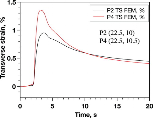
The two-step approach of experimentally measuring strain field and using a validated FE-based numerical model allows prediction of local critical stress/strain that leads to solidification cracking. As an example, the temporal evolution of transverse strain at a point P4 with coordinates (22.5, 10.5) mm, i.e. ∼ 1 mm from the fusion boundary was calculated using the validated FE-based numerical model (Figure 4). To compare, temporal transverse strain evolution at P2 is also plotted. As expected, at P4 the transverse strain is higher than that at P2.

Figure 4. FEM-computed temporal distribution of transverse strain (in %) at P2 and P4.

Summary

In summary, an approach to measure in situ strain fields on the top side of a welded specimen close to the fusion boundary is introduced. This method, based on external illumination and filters, allows measurement of strain fields with good spatial and temporal resolution as close as 1.5 mm from the fusion boundary. A validated FE-based numerical model can be useful in estimating local stress/strain conditions that prevail during welding. This model can be used to ascertain the strain/stress field in regions where laboratory experimental measurements are impractical.

Acknowledgments

The authors would like to thank the industrial partner in this project ‘Tata Steel Nederland B.V.’ for the financial support.

Disclosure statement

No potential conflict of interest was reported by the authors.

ORCID

G. Agarwal http://orcid.org/0000-0003-4669-7037

M. Amirthalingam http://orcid.org/0000-0001-9976-8922

M.J.M. Hermans http://orcid.org/0000-0002-6204-5285

Additional information

Funding

This research was carried out under project numbers F22.8.13485a and F22.8.13485b in the framework of the Partnership Program of the Materials innovation institute M2i (www.m2i.nl) and the Foundation for Fundamental Research on Matter (FOM) (www.fom.nl), which is part of the Netherlands Organisation for Scientific Research (www.nwo.nl).

References

- Kou S Welding metallurgy. John Wiley & Sons, Inc.; 2003. Available from: http://doi.org/10.1002/0471434027.ch7
- Kou S. A criterion for cracking during solidification. Acta Mater. 2015;88:366–374. Available from: http://www.scopus.com/inward/record.url?eid=2-s2.0-84923169994&partnerID=40&md5=3d73e0c7919371a6fec5da51e084d716 doi: 10.1016/j.actamat.2015.01.034
- Sutton MA, Orteu JJ, Schreier H. Image correlation for shape, motion and deformation measurements: basic concepts, theory and applications. 1st ed. Springer Publishing Company, Incorporated, New York; 2009.
- Kang J, Ososkov Y, Embury J, et al. Digital image correlation studies for microscopic strain distribution and damage in dual phase steels. Scr Mater. 2007;56(11):999–1002. Available from: https://www.scopus.com/inward/record.uri?eid=2-s2.0-34047181112&doi=10.1016%2fj.scriptamat.2007.01.031&partnerID=40&md5=5b1c0ba62542f8986e9238ec0f0e3b39 doi: 10.1016/j.scriptamat.2007.01.031
- Bumgardner C, Croom B, Li X. High-temperature delamination mechanisms of thermal barrier coatings: in-situ digital image correlation and finite element analyses. Acta Mater. 2017; Available from: http://www.sciencedirect.com/science/article/pii/S1359645417300873
- Limodin N, Réthoré J, Buffière JY, et al. Influence of closure on the 3D propagation of fatigue cracks in a nodular cast iron investigated by x-ray tomography and 3D volume correlation. Acta Mater. 2010;58(8):2957–2967. Available from: https://www.scopus.com/inward/record.uri?eid=2-s2.0-77949522004&doi=10.1016%2fj.actamat.2010.01.024&partnerID=40&md5=9086c01da4294df1b1aa88e979ac6bb9 doi: 10.1016/j.actamat.2010.01.024
- Gollnow C, Kannengiesser T. Hot cracking analysis using in situ digital image correlation technique. Weld World. 2013;57(3):277–284. Available from: http://doi.org/10.1007/s40194-013-0027-5
- De Strycker M, Lava P, Van Paepegem W, et al. Measuring welding deformations with the digital image correlation technique. Weld J. 2011;90(6):107S–112S.
- Shibahara M, Yamaguchi K, Onda T, et al. Studies on in-situ full-field measurement for in-plane welding deformation using digital camera. Weld Int. 2012;26(8):612–620. Available from: http://doi.org/10.1080/09507116.2011.592689 doi: 10.1080/09507116.2011.592689
- Chen X, Feng Z. In situ strain evaluation during tig welding determined by backside digital image correlation. Weld World. 2017;61(2):307–314. Available from: http://doi.org/10.1007/s40194-016-0410-0 doi: 10.1007/s40194-016-0410-0
- Aalderink B, Aarts R, Jonker J, et al. Weld plume emissions during nd:yag laser welding. In: Beyer E, Dausinger F, Ostendorf A, et al., editors. Lasers in manufacturing 2005. München” AT-Fachverlag GmbH Stuttgart; 2005. p. 413–417.
- VDEh. SEP 1220-3: testing and documentation guideline for the joinability of thin sheet of steel – part 3: laser beam welding; 2011.
- LIMESS webpage; 2017. Available from: http://www.limess.com/en/products/digital-image-correlation
- Shanmugam N, Buvanashekaran G, Sankaranarayanasamy K, et al. A transient finite element simulation of the temperature and bead profiles of T-joint laser welds. Mater Design. 2010;31(9):4528–4542. Available from: https://www.scopus.com/inward/record.uri?eid=2-s2.0-77953539095&doi=10.1016%2fj.matdes.2010.03.057&partnerID=40&md5=3fef3bf7669f2351a2e14fee56ea55e6 doi: 10.1016/j.matdes.2010.03.057
- ul abdein MZ, Nélias D, Jullien JF, et al. Experimental investigation and finite element simulation of laser beam welding induced residual stresses and distortions in thin sheets of AA 6056-T4. Mater Sci Eng: A. 2010;527(12):3025–3039. Available from: http://www.sciencedirect.com/science/article/pii/S0921509310000869 doi: 10.1016/j.msea.2010.01.054
- Gao H, Dutta RK, Huizenga RM, et al. Pass-by-pass stress evolution in multipass welds. Sci Technol Weld Joining. 2013;19(3):256–264. Available from: http://doi.org/10.1179/1362171813Y.0000000191 doi: 10.1179/1362171813Y.0000000191
- Feulvarch E, Robin V, Bergheau JM. Thermometallurgical and mechanical modelling of welding – application to multipass dissimilar metal girth welds. Sci Technol Weld Joining. 2013;16(3):221–231. Available from: http://doi.org/10.1179/1362171811Y.0000000008 doi: 10.1179/1362171811Y.0000000008
- Friedman E. Thermomechanical analysis of the welding process using the finite element method. J Press Vessel Technol. 1975;97(3):206–213. Available from: http://doi.org/10.1115/1.3454296 doi: 10.1115/1.3454296
- Karlsson RI, Josefson BL. Three-dimensional finite element analysis of temperatures and stresses in a single-pass butt-welded pipe. J Press Vessel Technol. 1990;112(1):76–84. Available from: http://doi.org/10.1115/1.2928591 doi: 10.1115/1.2928591
- Anca A, Cardona A, Risso J, et al. Finite element modeling of welding processes. Appl Math Model. 2011;35(2):688–707. Available from: http://www.sciencedirect.com/science/article/pii/S0307904X10002751 doi: 10.1016/j.apm.2010.07.026
- Ahmed EAA. Laser welding of advanced high strength steels [dissertation]. RWTH Aachen; 2011.
- Pan B, Qian K, Xie H, et al. Two-dimensional digital image correlation for in-plane displacement and strain measurement: a review. Measur Sci Technol. 2009;20(6):062001. Available from: http://stacks.iop.org/0957-0233/20/i=6/a=062001 doi: 10.1088/0957-0233/20/6/062001
- Shankar V, Gill TPS, Mannan SL, et al. Solidification cracking in austenitic stainless steel welds. Sadhana. 2003;28(3):359–382. Available from: http://doi.org/10.1007/BF02706438 doi: 10.1007/BF02706438
- Feng Z, David SA, Zacharia T, et al. Quantification of thermomechanical conditions for weld solidification cracking. Sci Technol Weld Joining. 2013;2(1):11–19. Available from: http://doi.org/10.1179/stw.1997.2.1.11 doi: 10.1179/stw.1997.2.1.11