Spurious Response Due to Linear Interpolation of Input Load and Some Remedies

ABSTRACT

This study focuses on the analytical identification and quantification of one type of spurious responses in the context of response history analysis. The spurious response is caused by linear interpolation of input loads. Through analytical derivations and numerical simulations, it is shown that the identified spurious response is fully caused by the interpolation and can significantly affect both damping and inertial forces. Furthermore, the spurious response is not bounded, thus, resistance-based designs could potentially be non-conservative. The findings are applicable to (non-)linear MDOF systems. To address this issue and improve the quality of numerical results, remedies and recommendations are proposed.

KEYWORDS:

• Response history analysis
• spurious structural response
• time integration
• digital signal processing
• dynamics

1. Introduction

Within a typical dynamic analysis workflow, various types of spurious responses stemming from different parts have been identified by researchers. To name a few,

1. error contained in the collected/applied input (Shing and Mahin 1987, Cui and Caracoglia 2016),

2. in the case of damped systems, the specific damping model used (Chrisp 1980, Carr 1997, Hall 2006, Jehel 2014, Chopra and McKenna 2015),

3. properties of the adopted numerical time integration method (associated with the spurious root and other factors) (Hulbert and Chung 1994, Cannillo and Mancuso 2000, Maheo, Rio, and Grolleau 2011, Maheo, Grolleau, and Rio 2012, Serfőző and Pere 2024).

Each process must be taken care of with great caution in order to obtain reasonable and reliable numerical results.

In the context of finite element response history analysis, seismic actions can be introduced into the system via either force or deformation. For the former, an acceleration record is converted to an inertial force with the assistance of a mass matrix and then applied to the target degrees of freedom. For the latter, a displacement record can be applied to supports to shake the structure as if it were on a shaking table. The typical sampling rate of ground motion seismograms ranges from 50 Hz to 200 Hz. This corresponds to a sampling period $T_s$ between 5 ms and 20 ms. When used as the time step size in response history analyses, such a value is often not sufficient for either linear or non-linear analysis due to accuracy and convergence issues, see, e.g., Chang (2011) and Rossi et al. (2014). Ideally, the continuous-time version of the input seismogram needs to be reconstructed from the discrete-time version in order to allow a smaller time step size to be used for simulation. However, the exact reconstruction is not achievable.

It is a convention to perform linear interpolation between two adjacent discrete samples when the time step size (of numerical analysis) is different from the sampling interval (of input seismogram). For example, ABAQUS (2014, see $\mathcal{\S }$ 34.1.2) provides functionalities to define loads in a tabular form, and the linear interpolation is automatically performed with optional smoothing within a small range ($\pm \mathit{\tau }$) around sharp turning points. Essentially, the linear interpolation is equivalent to a low-pass finite impulse response (FIR) filter with the Bartlett (triangular) window. Although the numerical error introduced by time integration methods and its impact on both linear and non-linear systems are well studied, see, e.g., Chang (2003, 2005), the side effect of such a linear interpolation procedure on numerical results is rarely discussed.

The present study investigates a particular type of spurious responses resulting from the linear interpolation of input force/deformation. The response is analysed analytically, providing clear evidence that the isolated error is entirely caused by interpolation and not by any other factors such as time integration methods. To quantify this error, analytical expressions for the damping and inertial forces of linear systems under interpolated or upsampled external loads are derived using signal processing methods. The corresponding transfer functions that relate the input ground motion and the output displacement/force response are plotted in the form of 2D figures to provide a direct visual approach to inspect the relative magnitude of the identified error. The results are then further elaborated upon using numerical simulations. To showcase the impact of this phenomenon on practical structures, a constrained cantilever under seismic loading is analysed. Remedies and recommendations to address this issue are also discussed. Finally, based on the discussions, a revised analysis workflow is proposed to improve the quality and reliability of numerical results of response history analyses.

2. Analytical Quantitation of Spurious Response

In this work, a continuous-time signal or function is denoted by lowercase letters, for example, $\mathit{u}\left(\mathit{t}\right)$. It’s duality in the frequency domain (via Fourier transform) is denoted with an overhead hat, for example, $\hat{u}\left(\mathit{\omega }\right)$ or $\hat{u}\left(\mathit{f}\right)$. A discrete-time signal is denoted by square brackets, for example, $\mathit{u}[\mathit{n}]$. The counterpart in the frequency domain (via the discrete Fourier transform) is denoted by uppercase letters, for example, $\mathit{U}[\mathit{n}]$. It can alternatively be approximated by sampling $\hat{u}\left(\mathit{\omega }\right)$ or $\hat{u}\left(\mathit{f}\right)$. The conversion between angular frequency $\mathit{\omega }$ and frequency $\mathit{f}$ is done implicitly.

2.1. Linear Interpolation

For the ease of discussion, let the sampling interval of an input seismogram be the multiple of time step size and let the ratio between them be an integer $\mathit{L}$. To apply the seismogram as an external load within each time step, interpolation is required, it is then equivalent to upsampling the input seismogram by the same ratio $\mathit{L}$. If the sampling rate/frequency of the original seismogram is $f_s$, then the upsampled signal has a sampling rate of $\mathit{L}{f}_s$. Extra attention shall be paid to the original Nyquist frequency $f_s/2$ since anything above it cannot be reliably reconstructed, due to, for example, aliasing. For a discrete-time signal $\mathit{p}[\mathit{n}]$, a typical upsampling operation with the upsampling factor $\mathit{L}$ consists of two steps (Oppenheim and Schafer 2010):

1. Insert $\mathit{L}-1$ zeros between each pair of adjacent samples in $\mathit{p}[\mathit{n}]$, resulting in a new signal $p_e[\mathit{n}]$ which can be formally defined as

   (1) $p_e[\mathit{n}]=\left\{\begin{array}{cc}\mathit{p}[\mathit{n}/\mathit{L}],& \mathit{n}=0,\mathit{L},2\mathit{L},3\mathit{L},\cdots ,\\ 0,& \mathrm{otherwise}.\end{array}\right.$(1)
   This is also known as an expander and is often denoted by $\uparrow \mathit{L}$ such that $p_e[\mathit{n}]=[\uparrow \mathit{L}]\mathit{p}[\mathit{n}]$.

2. Apply a low-pass filter with kernel $\mathit{g}[\mathit{n}]$ on $p_e[\mathit{n}]$ via convolution. The linear interpolation corresponds to the following kernel, often known as the Bartlett (triangular) window,

   (2) $\mathit{g}\left[\mathit{n}\right]=\left\{\begin{array}{cc}1-\left|\mathit{n}\right|/\mathit{L},& \left|\mathit{n}\right|\le \mathit{L}-1,\\ 0,& \mathrm{otherwise}.\end{array}\right.$(2)
   The convoluted/interpolated/filtered signal is denoted as $p_i[\mathit{n}]=\mathit{g}[\mathit{n}]\ast p_e[\mathit{n}]$. Different kernels will be discussed in subsequent sections.

Since the extended discrete signal $p_e[\mathit{n}]$ is $\mathit{p}[\mathit{n}]$ with additional zero samples, once the upsampling factor $\mathit{L}$ is chosen, $\mathit{p}[\mathit{n}]$ can be converted to $p_e[\mathit{n}]$ and vice versa. We focus on the properties of $p_e[\mathit{n}]$.

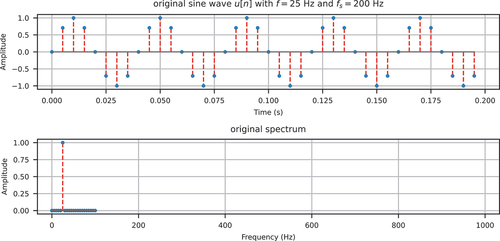
The bare $p_e[\mathit{n}]$ without applying any filter(s) contains spectral images, that is, extra copies of the original spectrum $\mathit{f}\in [0,f_s/2]$ in the additional frequency domain $\mathit{f}\in [f_s/2,\mathit{L}{f}_s/2]$. For example, consider the sinusoid

(3) $\mathit{u}(\mathit{t})=sin\left(2\mathit{\pi }{f}_0\mathit{t}\right),$(3)

with the frequency $f_0=\frac{{\omega }_0}{2\mathit{\pi }}$ chosen to be 25 Hz, a typical lower bound of processed seismograms. Assuming that this continuous-time signal is sampled at a rate of $f_s=200$ Hz, the discrete-time signal $\mathit{u}[\mathit{n}]$ can be depicted in Fig. 1.

Figure 1. Original sine wave in time domain and frequency domain.

The corresponding Nyquist frequency is $f_s/2=100$ Hz, thus, the frequency ranges from −100 Hz to 100 Hz (negative part not shown with amplitude of positive part properly scaled).

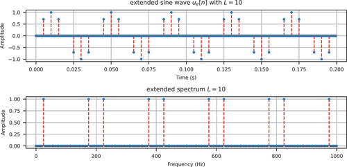
By choosing an upsampling factor $\mathit{L}=10$, the extended signal $u_e[\mathit{n}]$ (zero-stuffed/padded) can be illustrated as in Fig. 2.

Figure 2. Zero-stuffed sine wave in time domain and frequency domain.

The Nyquist frequency of $u_e[\mathit{n}]$ is $10\times 100\mathrm{Hz}=1000\mathrm{Hz}$, the original component at $25$ Hz is mirrored to $(200\pm 25)\mathrm{Hz},(400\pm 25)\mathrm{Hz},\left(600\pm 25\right)\mathrm{Hz},\left(800\pm 25\right)\mathrm{Hz}\mathrm{and}975\mathrm{Hz}$. Those additional components are known as images.

The linear interpolation (triangular window) for $\mathit{L}=10$ can be constructed as

(4) $\mathit{g}[\mathit{n}]=0.1\times \left[\begin{array}{ccccccccc}1& 2& 3& \cdots & 10& \cdots & 3& 2& 1\end{array}\right],$(4)

its frequency response $\mathit{G}[\mathit{n}]$ can be obtained via the discrete Fourier transform (DFT), which is shown in Fig. 3.

Figure 3. Triangular window in the frequency domain.

The analytical expression can be obtained via convoluting two rectangular signals, which gives

(5) $\hat{g}\left(\mathit{f}\right)=\sin {\mathrm{c}}^2\left(\frac{2\mathit{f}}{f_s}\right).$(5)

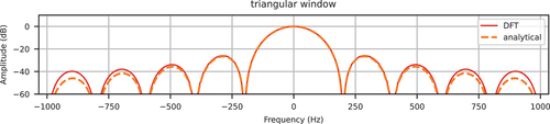
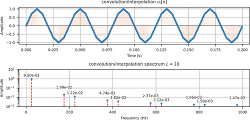
By the convolution theorem, the upsampled signal can be obtained by either convolution in the time domain or multiplication in the frequency domain. Fig. 4 shows the interpolated signal in both domains. Due to the high side lobe level (around −26 dB of the first side lobe, see Fig. 3) of the triangular window, the spectral images in $u_i[\mathit{n}]$ between 100 Hz and 1000 Hz are seemingly attenuated, for example, the component at 175 Hz is reduced to 1.99 × 10⁻², but their magnitudes are still relatively large. Using such an interpolated signal as the external load in dynamic analyses can sometimes cause significant spurious force responses, which are derived analytically in the following.

Figure 4. Interpolated sine wave in time domain and frequency domain.

2.2. Oscillator System

To investigate how the partially attenuated images would affect the response of oscillator systems, consider a single degree of freedom mass–spring–dashpot linear system under a harmonic load. The equation of motion can be written as

(6) $\mathit{ma}\left(\mathit{t}\right)+\mathit{cv}\left(\mathit{t}\right)+\mathit{ku}\left(\mathit{t}\right)=\mathit{p}\left(\mathit{t}\right),$(6)

with $\mathit{p}\left(\mathit{t}\right)=p_{0}sin\left(2\mathit{\pi ft}\right)$ where $p_0$ is the amplitude of the harmonic, and its angular frequency is $\mathit{\omega }=2\mathit{\pi f}$.

Duhamel’s integral shows the solution to this system can be expressed as, assuming trivial initial conditions,

(7) $\mathit{u}\left(\mathit{t}\right)=\left(\mathit{p}\ast \mathit{h}\right)\left(\mathit{t}\right)={\int }_0^t\mathit{p}\left(\mathit{\tau }\right)\mathit{h}\left(\mathit{t}-\mathit{\tau }\right)\mathit{d\tau },$(7)

with the fundamental solution

(8) $\mathit{h}\left(\mathit{t}\right)=\frac{1}{m{\omega }_d}exp\left(-\mathit{\zeta }{\omega }_n\mathit{t}\right)sin\left({\omega }_d\mathit{t}\right),$(8)

where $\mathit{m}$ is the mass, $\mathit{c}$ is the damping coefficient, $\mathit{k}$ is the stiffness, ${\omega }_n=\sqrt{\frac{k}{m}}$ is the natural frequency of the system, $\mathit{\zeta }=\frac{c}{2\sqrt{\mathit{mk}}}$ is the damping ratio, and ${\omega }_d={\omega }_n\sqrt{1-{\zeta }^2}$ is the damped frequency. The following discussion is confined to underdamped cases ($\mathit{\zeta }<1$).

Eq. (7)(7) $\mathit{u}\left(\mathit{t}\right)=\left(\mathit{p}\ast \mathit{h}\right)\left(\mathit{t}\right)={\int }_0^t\mathit{p}\left(\mathit{\tau }\right)\mathit{h}\left(\mathit{t}-\mathit{\tau }\right)\mathit{d\tau },$(7) can be conveniently evaluated in the frequency domain via the unilateral Laplace transform, see, e.g., Lee (1990), such that

(9) $\hat{u}\left(\mathit{\omega }\right)=\mathfrak{L}\left\{\mathit{u}\left(\mathit{t}\right)\right\}=\mathfrak{L}\left\{\mathit{p}\left(\mathit{t}\right)\right\}\cdot \mathfrak{L}\left\{\mathit{h}\left(\mathit{t}\right)\right\}=\hat{p}\left(\mathit{\omega }\right)\cdot \hat{h}\left(\mathit{\omega }\right),$(9)

with

(10) $\hat{h}\left(\mathit{\omega }\right)=\frac{1}{k}\frac{1}{\left(1-{\eta }^2\right)+\mathit{i}\left(2\mathit{\zeta \eta }\right)},\mathit{\eta }=\frac{\omega }{{\omega }_n}.$(10)

The velocity/acceleration spectrum can be obtained by differentiating $\hat{u}\left(\mathit{\omega }\right)$,

(11) $\hat{v}\left(\mathit{\omega }\right)=\mathit{i\omega }\cdot \hat{u}\left(\mathit{\omega }\right)=\mathit{i\omega }\cdot \hat{p}\left(\mathit{\omega }\right)\cdot \hat{h}\left(\mathit{\omega }\right),$(11)

(12) $\hat{a}\left(\mathit{\omega }\right)=\mathit{i\omega }\cdot \hat{v}\left(\mathit{\omega }\right)=-{\omega }^2\cdot \hat{p}\left(\mathit{\omega }\right)\cdot \hat{h}\left(\mathit{\omega }\right).$(12)

2.2.1. Damping Force

Denote the damping force as $F_v\left(\mathit{t}\right)=\mathit{cv}\left(\mathit{t}\right)$, then it is possible to derive

(13) ${\hat{F}}_{\mathit{v}}\left(\mathit{\omega }\right)=\mathfrak{L}\left\{F_v\left(\mathit{t}\right)\right\}=\mathit{c}\cdot \hat{v}\left(\mathit{\omega }\right)=\mathit{c}\cdot \mathit{i\omega }\cdot \hat{p}\left(\mathit{\omega }\right)\cdot \hat{h}\left(\mathit{\omega }\right).$(13)

We further denote

(14) ${\hat{k}}_{\mathit{v}}\left(\mathit{\omega }\right)=\mathit{ic\omega }\cdot \hat{h}\left(\mathit{\omega }\right),$(14)

which links the external load spectrum $\hat{p}\left(\mathit{\omega }\right)$ to the damping force spectrum ${\hat{F}}_{\mathit{v}}\left(\mathit{\omega }\right)$ such that

(15) ${\hat{F}}_{\mathit{v}}\left(\mathit{\omega }\right)={\hat{k}}_{\mathit{v}}\left(\mathit{\omega }\right)\cdot \hat{p}\left(\mathit{\omega }\right).$(15)

Now consider three different types of damping.

Constant Damping. Let $\mathit{c}$ (and $\mathit{\zeta }$) be a constant, accounting for Eq. (10)(10) $\hat{h}\left(\mathit{\omega }\right)=\frac{1}{k}\frac{1}{\left(1-{\eta }^2\right)+\mathit{i}\left(2\mathit{\zeta \eta }\right)},\mathit{\eta }=\frac{\omega }{{\omega }_n}.$(10) , then

(16) ${\hat{k}}_{\mathit{v}}\left(\mathit{\omega }\right)=\frac{\mathit{i}\left(2\mathit{\zeta \eta }\right)}{\left(1-{\eta }^2\right)+\mathit{i}\left(2\mathit{\zeta \eta }\right)}.$(16)

Mass Proportional Damping. Let $\mathit{c}$ be proportional to mass such that $\mathit{c}=2a_0\mathit{m}$, then

(17) $\mathit{\zeta }=\frac{2a_0\mathit{m}}{2\sqrt{\mathit{mk}}}=\frac{a_0}{{\omega }_n},\mathit{\zeta \eta }=\frac{a_0\mathit{\omega }}{{\omega }_n^2},$(17)

so that

(18) ${\hat{k}}_{\mathit{v}}\left(\mathit{\omega }\right)=\frac{i\left(2a_0\mathit{\omega }\right)}{\left({\omega }_n^2-{\omega }^2\right)+\mathit{i}\left(2a_0\mathit{\omega }\right)}.$(18)

Stiffness Proportional Damping. Let $\mathit{c}$ be proportional to stiffness such that $\mathit{c}=2a_1\mathit{k}$, then

(19) $\mathit{\zeta }=\frac{2a_1\mathit{k}}{2\sqrt{\mathit{mk}}}=a_1{\omega }_n,\mathit{\zeta \eta }=a_1\mathit{\omega },$(19)

so that

(20) ${\hat{k}}_{\mathit{v}}\left(\mathit{\omega }\right)=\frac{i\left(2a_1\mathit{\omega }\right)}{\left(1-{\eta }^2\right)+\mathit{i}\left(2a_1\mathit{\omega }\right)}.$(20)

It can be noticed that all three expressions of ${\hat{k}}_{\mathit{v}}\left(\mathit{\omega }\right)$ possess a similar form

(21) ${\hat{k}}_{\mathit{v}}\left(\mathit{\omega }\right)=\frac{\mathit{iA}}{\mathit{B}+\mathit{iA}}.$(21)

Note that $\mathit{B}=0$ when $\mathit{\omega }={\omega }_n$, correspondingly, ${\hat{k}}_{\mathit{v}}\left({\omega }_n\right)=1$, which is the maximum magnitude of ${\hat{k}}_{\mathit{v}}\left(\mathit{\omega }\right)$. At this point, the magnitude of the damping force component simply equals that of the external load component, see Eq. (15)(15) ${\hat{F}}_{\mathit{v}}\left(\mathit{\omega }\right)={\hat{k}}_{\mathit{v}}\left(\mathit{\omega }\right)\cdot \hat{p}\left(\mathit{\omega }\right).$(15) . With that said, although the damping ratio either decays to zero asymptotically (mass proportional) or grows to infinity (stiffness proportional), the corresponding damping force is bounded, the maximum of which depends on the magnitude of the external load at resonance ($\mathit{\omega }={\omega }_n$).

For those three cases, ${\hat{k}}_{\mathit{v}}\left(\mathit{\omega }\right)$ can be computed and illustrated in Figs. 5–7 for different $f_n$ (or equivalently, ${\omega }_n$). From those figures, one could infer that, if the external load has relatively large components around the natural frequency of the system, the resulting damping force could potentially be large. Such large components can be caused by the aforementioned images due to linear interpolation.

Figure 5. Fundamental solutions with constant damping.

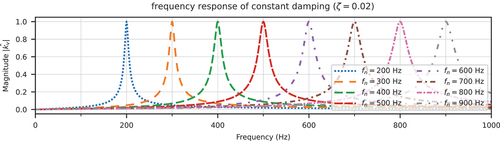
Figure 6. Fundamental solutions with stiffness proportional damping.

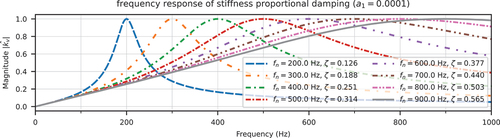
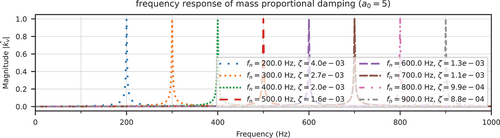
Figure 7. Fundamental solutions with mass proportional damping.

Since the external load $\mathit{p}\left(\mathit{t}\right)$ would be discretised for numerical analysis, it is possible to move the interpolation filter $\hat{g}\left(\mathit{f}\right)$ to ${\hat{k}}_{\mathit{v}}\left(\mathit{f}\right)$, we further denote the product by

(22) ${\hat{m}}_{\mathit{v}}\left(\mathit{f}\right)=\hat{g}\left(\mathit{f}\right)\cdot {\hat{k}}_{\mathit{v}}\left(\mathit{f}\right),$(22)

such that

(23) ${\hat{F}}_{\mathit{v}}\left(\mathit{f}\right)={\hat{m}}_{\mathit{v}}\left(\mathit{f}\right)\cdot {\hat{p}}_{\mathit{e}}\left(\mathit{f}\right),$(23)

where ${\hat{p}}_{\mathit{e}}\left(\mathit{f}\right)$ is the spectrum of extended (zero-stuffed) external load that possesses identical magnitude at imaging frequencies, see Fig. 2.

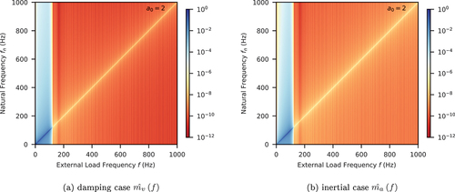
The above ${\hat{m}}_{\mathit{v}}\left(\mathit{f}\right)$ can be treated as the transfer function between external load (input) and damping force (output). It reveals the magnitudes of the damping force for any given frequency component of the external load. It is then possible to plot the magnitude of ${\hat{m}}_{\mathit{v}}\left(\mathit{f}\right)$ in the frequency domain by choosing different natural frequencies $f_n$ and damping model parameters. One example is given in Fig. 8.

Figure 8. Magnitude of ${\hat{m}}_{\mathit{v}}\left(\mathit{f}\right)$ for $f_n=200$Hz with $a_1=0.0001$.

The analytical expression of ${\hat{m}}_{\mathit{v}}\left(\mathit{f}\right)$ provides a convenient tool to query the magnitude of the damping force in a given system. For example, if the upsampled sine wave in Fig. 2 is used as the external load, it has a 25 Hz component with a magnitude of 1, then the damping force shall have the same component of a magnitude $1\times 3.03\times {10}^{-2}$. The factor 3.03 × 10⁻² is obtained by computing the magnitude of ${\hat{m}}_{\mathit{v}}\left(\mathit{f}\right)$ at $\mathit{f}=25$Hz (see Fig. 8). Similarly, the 225 Hz component shall have a magnitude of 8.91 × 10⁻³.

2.2.2. Inertial Force

Similarly, the inertial force can be derived as

(24) ${\hat{F}}_{\mathit{a}}\left(\mathit{f}\right)={\hat{p}}_{\mathit{e}}\left(\mathit{f}\right)\cdot {\hat{m}}_{\mathit{a}}\left(\mathit{f}\right),{\hat{m}}_{\mathit{a}}\left(\mathit{f}\right)=\hat{g}\left(\mathit{f}\right)\cdot {\hat{k}}_{\mathit{a}}\left(\mathit{f}\right),$(24)

where

(25) ${\hat{k}}_{\mathit{a}}\left(\mathit{\omega }\right)=-\mathit{m}{\omega }^2\cdot \hat{h}\left(\mathit{\omega }\right)=\frac{-{\eta }^2}{\left(1-{\eta }^2\right)+\mathit{i}\left(2\mathit{\zeta \eta }\right)}.$(25)

For the stiffness/mass proportional damping, $\mathit{\zeta }$ takes the same expressions, viz., $a_1{\omega }_n$ and $a_0/{\omega }_n$, respectively.

2.2.3. Remarks

We derive the transfer functions ${\hat{m}}_{\mathit{v}}\left(\mathit{f}\right)$ and ${\hat{m}}_{\mathit{a}}\left(\mathit{f}\right)$ between the zero-stuffed input (external load) and the output (damping/inertial force) as follows.

(26) ${\hat{m}}_{\mathit{v}}\left(\mathit{f}\right)=\hat{g}\left(\mathit{f}\right)\cdot {\hat{k}}_{\mathit{v}}\left(\mathit{f}\right),$(26)

(27) ${\hat{m}}_{\mathit{a}}\left(\mathit{f}\right)=\hat{g}\left(\mathit{f}\right)\cdot {\hat{k}}_{\mathit{a}}\left(\mathit{f}\right).$(27)

The filter kernel $\hat{g}\left(\mathit{f}\right)$ can take various forms, depending on the specific type of filters chosen. For linear interpolation (triangular window), it possesses the analytical expression as shown in Eq. (5)(5) $\hat{g}\left(\mathit{f}\right)=\sin {\mathrm{c}}^2\left(\frac{2\mathit{f}}{f_s}\right).$(5) . The terms ${\hat{k}}_{\mathit{v}}\left(\mathit{f}\right)$ and ${\hat{k}}_{\mathit{a}}\left(\mathit{f}\right)$ also take various forms, as shown in Eq. (16)(16) ${\hat{k}}_{\mathit{v}}\left(\mathit{\omega }\right)=\frac{\mathit{i}\left(2\mathit{\zeta \eta }\right)}{\left(1-{\eta }^2\right)+\mathit{i}\left(2\mathit{\zeta \eta }\right)}.$(16) , Eq. (18)(18) ${\hat{k}}_{\mathit{v}}\left(\mathit{\omega }\right)=\frac{i\left(2a_0\mathit{\omega }\right)}{\left({\omega }_n^2-{\omega }^2\right)+\mathit{i}\left(2a_0\mathit{\omega }\right)}.$(18) , Eq. (20)(20) ${\hat{k}}_{\mathit{v}}\left(\mathit{\omega }\right)=\frac{i\left(2a_1\mathit{\omega }\right)}{\left(1-{\eta }^2\right)+\mathit{i}\left(2a_1\mathit{\omega }\right)}.$(20) and Eq. (25)(25) ${\hat{k}}_{\mathit{a}}\left(\mathit{\omega }\right)=-\mathit{m}{\omega }^2\cdot \hat{h}\left(\mathit{\omega }\right)=\frac{-{\eta }^2}{\left(1-{\eta }^2\right)+\mathit{i}\left(2\mathit{\zeta \eta }\right)}.$(25) , depending on the type of damping used.

It shall be emphasised that the above discussion is purely analytical, without potential numerical errors introduced by various numerical time integrations and other similar approximations. The transfer functions ${\hat{m}}_{\mathit{v}}\left(\mathit{f}\right)$ and ${\hat{m}}_{\mathit{a}}\left(\mathit{f}\right)$ essentially reveal how the imaging frequencies existing in the input would eventually affect the output response. Thus, they can be used as indicators of errors solely stemming from upsampling/interpolation of the input load.

One can compute ${\hat{m}}_{\mathit{v}}\left(\mathit{f}\right)$ and ${\hat{m}}_{\mathit{a}}\left(\mathit{f}\right)$ over the whole frequency domain for different damping models and upsampling filters, and compare the relative magnitudes between two regions, in the case of the chosen signal, $\mathit{f}\in [0\mathrm{Hz},100\mathrm{Hz}]$ and $\mathit{f}\in [100\mathrm{Hz},1000\mathrm{Hz}]$, to evaluate if the images could lead to significant spurious responses.

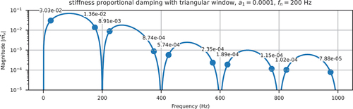
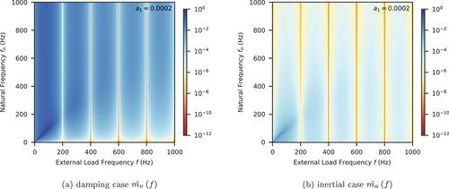
Two examples are presented as follows. In Fig. 9, the triangular window (linear interpolation) with $\mathit{L}=10$ is chosen with a constant damping ratio $\mathit{\zeta }=0.02$. In Fig. 10, the triangular window with $\mathit{L}=10$ is chosen with a stiffness proportional damping $a_1=2\times {10}^{-4}$. In both examples, it is clearly seen that the undesired response at frequencies ranging between 100 Hz and 1000 Hz (that do not exist in the original signal, see Fig. 1) is poorly attenuated, the magnitude of which is comparable to that of the original signal ($[0\mathrm{Hz},100\mathrm{Hz}]$) as both share similar colours. This introduces the risk of unreliable/unusable numerical results.

Figure 9. Normalised damping/inertial force magnitude with constant damping ratio and triangular window.

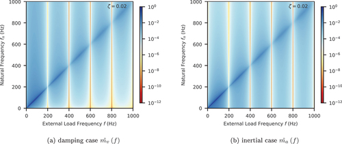
Figure 10. Normalised damping/inertial force magnitude with stiffness proportional damping and triangular window.

To suppress such a spurious response, ${\hat{m}}_{\mathit{v}}\left(\mathit{f}\right)$ and ${\hat{m}}_{\mathit{a}}\left(\mathit{f}\right)$ must have significantly small magnitudes beyond the original Nyquist frequency (100 Hz for the particular example used).

Alternatively, the whole system can be deemed as a stochastic system, with components at imaging frequencies treated as errors, and analysed accordingly, see, e.g., Söderström (2002).

2.3. A Preliminary Example

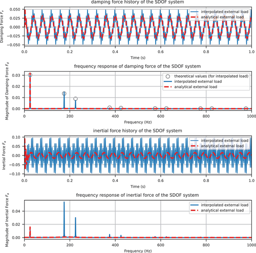
The concept is best validated via a simple example. A linear single degree of freedom system is modelled with the following parameters.

(28) $f_n=200,\mathit{m}=1,\mathit{k}=4{\pi }^2{f}_n^2=1.579\times {10}^6,a_1={10}^{-4},\mathit{c}=2a_1\mathit{k}=315.827,$(28)

with the external load and time step size

(29) $\mathit{p}\left(\mathit{t}\right)=sin\left(50\mathit{\pi t}\right),\mathrm{\Delta t}=5\times {10}^{-4}.$(29)

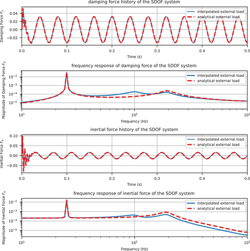
For comparison, the external load is provided in two forms:

1. sampled at 200 Hz and upsampled to 2000 Hz as shown in Fig. 4 — this is the conventional approach which introduces spurious response, and

2. analytically evaluated at each time point — this is analytical such that it only contains one component at 25 Hz as shown in Fig. 1.

The damping/inertial force history and its frequency components are shown in Fig. 11.

Figure 11. Damping/inertial force history and spectrum of the SDOF system (transient solution included) using triangular window and Newmark method with $\mathit{\gamma }=0.5$ and $\mathit{\beta }=0.25$.

The interpolated external load contains relatively large imaging frequencies and results in significant overshoots (around 50% for damping force and around 500% for inertial force) due to significant components at 175 Hz and 225 Hz, which are not attenuated by the linear interpolation. The values agree with Fig. 8.

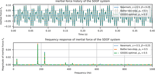
It must be re-emphasised that, as stated in the previous remarks, the identified spurious response stems from the input, instead of the numerical time integration. Thus, it can be analytically isolated. As a result, no matter how “good” the adopted time integration method is, the spurious response can always be observed. Fig. 12 shows the inertial force history and spectrum using various time integration algorithms. It can be seen that all methods show spikes at imaging frequencies.

Figure 12. Inertial force history and spectrum of the SDOF system (transient solution included) using interpolated external load and various time integration methods.

Given that numerical models inevitably contain high-frequency modes due to, for example, finite element discretisation and the presence of constraints implemented via the penalty function method, the contribution of high-frequency components to damping/inertial force can be amplified significantly. It must be emphasised that according to Eq. (21)(21) ${\hat{k}}_{\mathit{v}}\left(\mathit{\omega }\right)=\frac{\mathit{iA}}{\mathit{B}+\mathit{iA}}.$(21) , as long as damping is considered, no matter which type, the maximum possible magnitude of damping force of a specific frequency is equal to that of the upsampled (after filtering) external load. Furthermore, it is also independent of the magnitude of damping, small or large. In fact, a large damping ratio gives flat ${\hat{k}}_{\mathit{v}}\left(\mathit{f}\right)$, which reduces the difference between low-frequency response and high-frequency response. It is thus less likely to overshoot regarding damping force alone. It can also be concluded that, as long as the damping model is not point-based (for example, the Wilson–Penzien model, which only responds to selected discrete frequencies), the system is not immune from spurious damping forces. It is also evident from analytical expressions that as long as mass is not zero, the inertial force would be affected by this type of spurious response.

In the case of multiple degrees of freedom (MDOF) systems, depending on the distribution of natural frequencies and the composition of the external load, as well as the upsampling ratio, higher modes may produce significant responses due to, for example, being closer to imaging frequencies. The final numerical results may contain a considerably large portion of spurious responses.

2.4. A Note on Load Applied as Displacement

In the previous example, we illustrate the spurious response caused by the linear interpolation in the context of load being applied as (inertial) force. In some displacement–controlled applications, external loads can be applied in the form of deformation. Two options are typically available: 1) directly apply the recorded displacement to the target DoFs, or 2) convert recorded acceleration to displacement by integration and apply it to the target DoFs. The first approach is not immune to the spurious response as long as linear interpolation is used. The second approach is thus preferred.

3. Remedies and Recommendations

As can be seen in Fig. 11, using the analytical expression for the external load is clearly a solution that can fully suppress spurious response. However, this is not a feasible option as analytical expressions of seismograms cannot be reconstructed easily. The following remedies and recommendations are proposed to mitigate the issue.

3.1. Low-pass Filters with Better Attenuation

If the oscillator system is deemed as a filter system, it is evident that the fundamental cause of spurious forces is the high-frequency noise in the input. A natural remedy is to suppress high-frequency components as much as possible. In this regard, the linear interpolation is error-prone. Other options are available.

Ideally, a low-pass filter with a high roll-off rate and a low side lobe level can suppress the images caused by upsampling to the level that the corresponding spurious responses will not have a significant impact on final numerical results, even after scaling up by a factor of ${\omega }^2$.

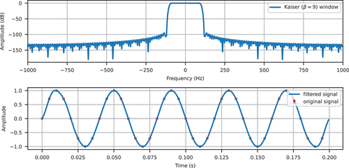
We show a number of different windows in Figs. 13–15, including the Blackman–Nuttall window, the flat top window, and the Kaiser family. Those are commonly used windows (Oppenheim and Schafer, 2010) in the design of FIR filters. The number of bins is chosen to be $32\mathit{L}+1$ ($\mathit{L}=10$ in this work) to obtain a side lobe level around −100 dB.

Figure 13. Blackman–Nuttall window and the filtered signal.

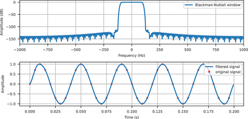
Figure 14. Flat top window and the filtered signal.

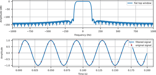
Figure 15. Kaiser window ($\mathit{\beta }=9$) and the filtered signal.

With those windows, it is possible to repeat the previous procedure to obtain distributions of ${\hat{m}}_{\mathit{v}}$ and ${\hat{m}}_{\mathit{a}}$ that reveal the relative magnitudes of damping and inertial forces. Fig. 16–21 show the examples with three different types of damping models for Kaiser and Blackman-Nuttall windows, respectively. It is evident that imaging frequencies can be greatly attenuated, even on the resonance line ($\mathit{f}=f_n$). By comparing colours in those figures, it can be seen that the responses beyond the original Nyquist frequency 100 Hz are significantly smaller by around four to six orders of magnitude.

Figure 16. Normalised damping/inertial force magnitude with constant damping ratio and Kaiser window.

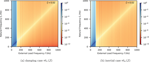
Figure 17. Normalised damping/inertial force magnitude with stiffness proportional damping and Kaiser window.

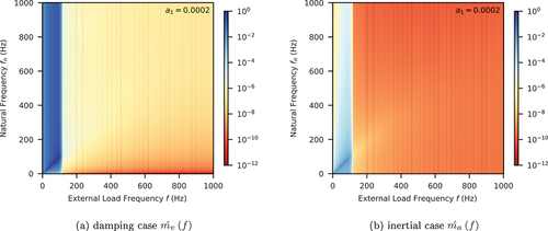
Figure 18. Normalised damping/inertial force magnitude with mass proportional damping and Kaiser window.

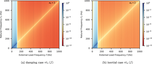
Figure 19. Normalised damping/inertial force magnitude with constant damping ratio and Blackman–Nuttall window.

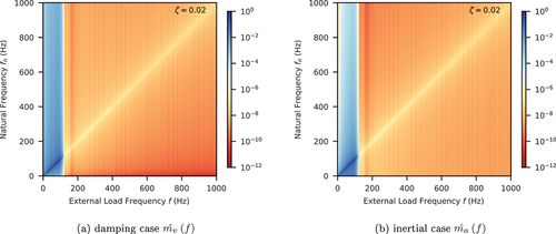
Figure 20. Normalised damping/inertial force magnitude with stiffness proportional damping and Blackman–Nuttall window.

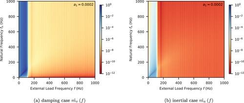
Figure 21. Normalised damping/inertial force magnitude with mass proportional damping and Blackman–Nuttall window.

If such a spurious response has to be suppressed to a level under −40 dB, which corresponds to 1%, it is possible to estimate the required side lobe level by using the upsampled Nyquist frequency $\mathit{L}{f}_s/2$ such that

(30) $20log\left(\frac{0.01}{{\left(\frac{L{f}_s}{2}\right)}^2}\right)=20log\left(\frac{0.04}{L^2{f}_s^2}\right).$(30)

For $\mathit{L}{f}_s=100$Hz, this gives −108 dB. For $\mathit{L}{f}_s=500$Hz, this gives −136 dB.

3.2. Other Recommendations

3.2.1. Avoid Upsampling/interpolation

The additional frequencies beyond the original Nyquist frequency stem from upsampling. If the input can be expressed analytically, such as modulated periodic signals that can be decomposed into simple sinusoids/exponentials, it is recommended to compute its magnitude analytically. This approach, though not always feasible, would be completely free from imaging.

3.2.2. Better Interpolation

Generally speaking, low-pass FIR filters cannot retain the exact magnitudes of the original samples. This is not considered a major issue as it is likely that the digital seismogram at hand is already preprocessed via some band-pass filter.

Alternatively, other interpolations can be used. Lee (1989) discussed a number of methods of different orders. The cubic spline interpolation (see Burden and Douglas 2011, $\mathcal{\S }$ 3.5) is another better alternative to the linear interpolation.

3.2.3. Time Integration with Algorithmic Damping

It is widely accepted by the community that the presence of algorithmic damping (with the proper amount properly distributed) is beneficial. Algorithmic damping can partially reduce spurious responses, see, e.g., Maheo, Rio, and Grolleau (2011), Mirbagheri et al. (2015) and Serfőző and Pere (2024). It is able to improve the quality of numerical results of simulations of structural dynamics and wave propagation problems. However, it is not effective when it comes to suppressing the spurious response discussed in this work. The following presents a brief discussion on this matter.

For a specific time integration method, one can derive the corresponding numerical transfer function that approximates the theoretical one Eq. (10)(10) $\hat{h}\left(\mathit{\omega }\right)=\frac{1}{k}\frac{1}{\left(1-{\eta }^2\right)+\mathit{i}\left(2\mathit{\zeta \eta }\right)},\mathit{\eta }=\frac{\omega }{{\omega }_n}.$(10) . Preumont (1982) presented an analysis of several time integration methods in the frequency domain and derived the corresponding transfer functions. Arias-Trujillo et al. (2012) carried out similar research and benchmarked a number of different time integration algorithms. Relevant methodology is directly adopted in this work. One can plot the ratio between numerical and analytical transfer functions. Fig. 22 shows the ratio between numerical (${\hat{h}}_{\mathit{NM}}$, Newmark method) and theoretical ($\hat{h}$) transfer functions. As can be seen, with a proper set of parameters, high-frequency responses (around resonance and onwards) can be suppressed by algorithmic damping. However, it is noticed that spurious responses could be several orders of magnitude larger than responses at low frequencies, especially for inertial forces, the roll-off rate of algorithmic damping is not great enough to sufficiently suppress spurious responses. One must be aware of the fact that the numerical integration error increases as $\mathit{f}\Delta \mathit{t}$ increases. Thus, results closer to the upsampled Nyquist frequency $\mathit{L}{f}_s/2$ contain significant errors that may suppress high-frequency responses in some cases, or amplify them in others. Time integration methods with better accuracy are always preferred.

Figure 22. ratio between numerical and analytical transfer functions ($\mathrm{\Delta t}=0.005$ and $\mathit{\zeta }=0.05$).

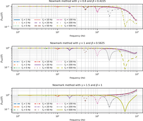
The Newmark method only possesses a first-order accuracy when $\mathit{\gamma }>0.5$, other methods are more favourable. Among them, the GSSSS framework (Zhou and Tamma 2003, 2006) and the Bathe two-step method (Noh and Bathe 2019), representing two major categories, are recommended. They are second-order accurate and provide controllable algorithmic damping.

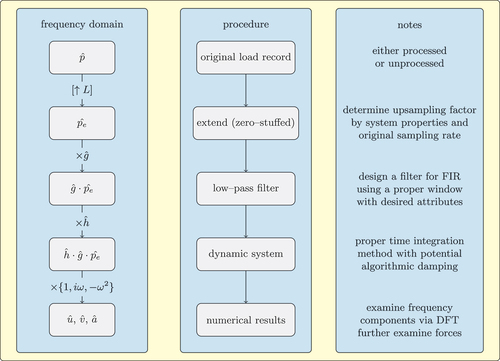
3.3. A Revised Workflow

Based on the above discussions, a revised workflow for response history analysis is proposed and summarised in Fig. 23. Analysts are suggested to filter input seismograms before performing analyses and examine numerical results in the frequency domain.

Figure 23. Typical analysis flow with recommendations.

4. Numerical Examples

4.1. Improved SDOF Example

Fig. 24 presents the results of the same SDOF system described in $\mathcal{\S }$ 2.3 but with the Blackman–Nuttall window (see Fig. 13) and the generalised-$\mathit{\alpha }$ time integration method, while all other configurations remain unchanged.

Figure 24. Damping/inertial force history and spectrum of the SDOF system (transient solution included) using Blackman–Nuttall window and the generalised-$\mathit{\alpha }$ time integration method with ${\rho }_{\mathrm{\infty }}=0.5$.

It is evident that with better attenuations at imaging frequencies, the quality of numerical results is greatly improved, which allows more accurate and confident interpretation.

4.2. A Cantilever Wall

We present one more example of a cantilever wall under seismic load. The model, as well as the corresponding configurations, are depicted in Fig. 25.

Figure 25. A simple cantilever wall example.

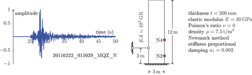
The accelerogram is sampled at 50 Hz, while the time step size for numerical analysis is chosen to be 4. This requires an upsampling factor of $\mathit{L}=5$. Two filter windows are used: 1) triangular window (linear interpolation) and 2) Blackman–Nuttall window. All other parameters are identical in two analyses.

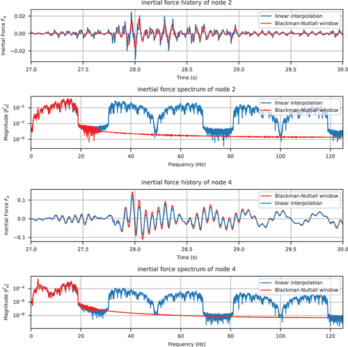
Fig. 26 shows the inertial force history of nodes 2 and 4. Due to the presence of the rigid link, the numerical model contains high-frequency components, which mainly affect the lower part (below the rigid link) of the wall. The imaging frequencies caused by linear interpolation show significant contributions to the inertial force history at node 2. As a result, it exhibits a larger profile compared to its counterpart using the Blackman–Nuttall window. The response of the upper part (above the rigid link) of the wall is mainly dominated by low-frequency modes, causing a smaller profile, as can be seen in the inertial force history of node 4. Although it may appear difficult to determine which result is more accurate/reliable at first glance, from the aforementioned discussion, it can be confidently concluded that the response due to the filtered (via the Blackman–Nuttall window) ground motion is more reliable. According to Rayleigh’s energy theorem, compared to the linear interpolated version, the total energy represented by the filtered record is closer to that of the original record.

Figure 26. Inertial force history and spectrum Blackman–Nuttall window.

In general, it is not feasible to predict whether imaging frequencies would cause significant discrepancy in the dynamic response of oscillating systems, let alone to quantitatively determine its magnitude, as it could be affected by many factors, including various properties of both input loads and the system. As a universal pre-processing protocol, it is thus recommended to always use a proper filter to filter the ground motion record before performing any response history analyses.

5. Conclusions

In this work, we demonstrate and analytically quantify one type of spurious responses existing in both linear and non-linear dynamic analysis of vibrating systems that stems from linear interpolation of input loads, which may be collected from sampling instruments such as actuators and seismometers. Within the scope of seismic engineering, typical values are chosen to illustrate the issue. It is worth emphasising that the identified issue is not applicable to systems in which the input is exact but does exist in all other systems as long as linear interpolation is used, regardless of parameters (sampling frequency of input, material properties of system, natural frequency distribution, etc.).

Through examples, it is concluded that the linear interpolation is neither ideal nor reliable. The following recommendations are made.

1. In order to avoid linear interpolation, it is better to have an identical time step size and sampling interval. To this end, analysts shall first choose a proper time step size that would be used in numerical analysis. Typically, it is smaller than the sampling interval of ground motions and is determined by the property of the dynamic system of interest. Then, the seismogram shall be processed by upsampling. A low-pass filter with sufficiently small side lobe level shall be applied to suppress any components above the original Nyquist frequency.

2. The high-frequency noise exists intrinsically and can be isolated analytically. Algorithmic damping can alleviate the issue but only to a limited degree; nevertheless, it is still beneficial to adopt a time integration method with adjustable algorithmic damping. In this regard, the de facto Newmark method, which is widely used, is not recommended.

Based on the above recommendations, the following workflow is proposed for conventional response history analysis.

1. Determine whether the seismograph, in the form of either displacement or acceleration, is properly processed. Typical seismographs are preprocessed by applying a band-pass filter with bounds at around 0.05 Hz and 25 Hz to 50 Hz for structural analysis, see, e.g., Houtte et al. (2017).

2. Determine the proper time step size and thus the corresponding upsampling ratio.

3. Design a proper upsampling filter so that the time step size matches the upsampling interval.

4. Avoid high-frequency modes in the target structure. Constraints can be better implemented via the Lagrange multiplier method.

5. Perform analysis using filtered records and a time integration method with adjustable algorithmic damping.

6. Examine the final results to ensure there are no significant high-frequency components.

For software vendors, in addition to de facto linear interpolation, extra options shall be provided when it comes to processing tabular data. Unless the desired load can be accurately represented in a tabular form, in the absence of an explicitly defined processing of the input load, a default upsampling procedure with proper filter parameters can be applied.

The numerical examples are carried out using suanPan (Chang 2022). Scripts to generate figures and models can be found online.¹

Disclosure Statement

No potential conflict of interest was reported by the author(s).

Data Availability Statement

Data will be made available on request.

Notes

1. https://github.com/TLCFEM/dsp-dynamics.

References

- ABAQUS. 2014. Analysis User’s Guide Volume V: Prescribed Conditions, Constraints & Interactions. Providence, RI: Dassault Systèmes.
- Arias-Trujillo, J., R. Blázquez, and S. López-Querol. 2012. “A Methodology Based on a Transfer Function Criterion to Evaluate Time Integration Algorithms.” Soil Dynamics and Earthquake Engineering 37:1–23. https://doi.org/10.1016/j.soildyn.2012.01.008.
- Burden, R. L., and F. J. Douglas. 2011. Numerical Analysis. 9th ed. Boston, MA: Brooks/Cole, Cengage Learning.
- Cannillo, V., and M. Mancuso. 2000. “Spurious Resonances in Numerical Time Integration Methods for Linear Dynamics.” Journal of Sound and Vibration 238 (3): 389–399. https://doi.org/10.1006/jsvi.2000.3104.
- Carr, A. J. 1997. “Damping Models for Inelastic Analyses.” Proceedings of the Asia-Pacific Vibration Conference, 42–48. Kyongju, Korea.
- Chang, T. L. 2022. Suanpan — an Open Source, Parallel and Heterogeneous Finite Element Analysis Framework. https://doi.org/10.5281/ZENODO.1285221.
- Chang, S.-Y. 2003. “Nonlinear Error Propagation Analysis for Explicit Pseudodynamic Algorithm.” Journal of Engineering Mechanics 129 (8): 841–850. https://doi.org/10.1061/(ASCE)0733-9399.
- Chang, S.-Y. 2005. “Error Propagation in Implicit Pseudodynamic Testing of Nonlinear Systems.” Journal of Engineering Mechanics 131 (12): 1257–1269. https://doi.org/10.1061/(ASCE)0733-9399.
- Chang, S.-Y. 2011. “Selection of Time Step for Pseudodynamic Testing.” Earthquake Engineering and Engineering Vibration 10 (3): 437–451. https://doi.org/10.1007/s11803-011-0079-8.
- Chopra, A. K., and F. McKenna. 2015. “Modeling Viscous Damping in Nonlinear Response History Analysis of Buildings for Earthquake Excitation.” Earthquake Engineering & Structural Dynamics 45 (2): 193–211. https://doi.org/10.1002/eqe.2622.
- Chrisp, D. J. 1980. Damping Models for Inelastic Structures, mathesis. NZ: University of Canterbury.
- Cui, W., and L. Caracoglia. 2016. “Physics-Based Method for the Removal of Spurious Resonant Frequencies in High-Frequency Force Balance Tests.” Journal of Structural Engineering 142 (2). https://doi.org/10.1061/(asce)st.1943-541x.0001414.
- Hall, J. F. 2006. “Problems Encountered from the Use (Or Misuse) of Rayleigh Damping.” Earthquake Engineering & Structural Dynamics 35 (5): 525–545. https://doi.org/10.1002/eqe.541.
- Houtte, C. V., S. Bannister, C. Holden, S. Bourguignon, and G. McVerry. 2017. “The New Zealand Strong Motion Database.” Bulletin of the New Zealand Society for Earthquake Engineering 50 (1): 1–20. https://doi.org/10.5459/bnzsee.50.1.1-20.
- Hulbert, G. M., and J. Chung. 1994. “The Unimportance of the Spurious Root of Time Integration Algorithms for Structural Dynamics.” Communications in Numerical Methods in Engineering 10 (8): 591–597. https://doi.org/10.1002/cnm.1640100803.
- Jehel, P. 2014. “A Critical Look into Rayleigh Damping Forces for Seismic Performance Assessment of Inelastic Structures.” Engineering Structures 78:28–40. https://doi.org/10.1016/j.engstruct.2014.08.003.
- Lee, V. W. 1989. “Recent Developments on Data Processing of Strong-Motion Accelerograms: Interpolation of Uniform and Non-Uniform Sampling from Digitized Acceleration Data.” Soil Dynamics and Earthquake Engineering 8 (4): 202–212. https://doi.org/10.1016/s0267-7261(89)80021-1.
- Lee, V. W. 1990. “Efficient Algorithm for Computing Displacement, Velocity and Acceleration Responses of an Oscillator to Arbitrary Ground Motion.” Soil Dynamics and Earthquake Engineering 9 (6): 288–300. https://doi.org/10.1016/s0267-7261(05)80015-6.
- Maheo, L., V. Grolleau, and G. Rio. 2012. “Numerical Damping of Spurious Oscillations: A Comparison Between the Bulk Viscosity Method and the Explicit Dissipative Tchamwa–Wielgosz Scheme.” Computational Mechanics 51 (1): 109–128. https://doi.org/10.1007/s00466-012-0708-8.
- Maheo, L., G. Rio, and V. Grolleau. 2011. “On the Use of Some Numerical Damping Methods of Spurious Oscillations in the Case of Elastic Wave Propagation.” Mechanics Research Communications 38 (2): 81–88. https://doi.org/10.1016/j.mechrescom.2011.01.006.
- Mirbagheri, Y., H. Nahvi, J. Parvizian, and A. Düster. 2015. “Reducing Spurious Oscillations in Discontinuous Wave Propagation Simulation Using High-Order Finite Elements.” Computers & Mathematics with Applications 70 (7): 1640–1658. https://doi.org/10.1016/j.camwa.2015.06.022.
- Noh, G., and K.-J. Bathe. 2019. “The Bathe Time Integration Method with Controllable Spectral Radius: The ρ∞-Bathe Method.” Computers & Structures 212:299–310. https://doi.org/10.1016/j.compstruc.2018.11.001.
- Oppenheim, A. V., and R. W. Schafer. 2010. Discrete-Time Signal Processing. 3rd ed. Upper Saddle River, NJ: Pearson.
- Preumont, A. 1982. “Frequency Domain Analysis of Time Integration Operators.” Earthquake Engineering & Structural Dynamics 10 (5): 691–697. https://doi.org/10.1002/eqe.4290100506.
- Rossi, D. F., W. G. Ferreira, W. J. Mansur, and A. F. G. Calenzani. 2014. “A Review of Automatic Time-Stepping Strategies on Numerical Time Integration for Structural Dynamics Analysis.” Engineering Structures 80:118–136. https://doi.org/10.1016/j.engstruct.2014.08.016.
- Serfőző, D., and B. Pere. 2024. “An Effective Reduction Method with Caughey Damping for Spurious Oscillations in Dynamic Problems.” https://doi.org/10.21203/rs.3.rs-3930320/v1.
- Shing, P.-S. B., and S. A. Mahin. 1987. “Elimination of Spurious Higher-Mode Response in Pseudodynamic Tests.” Earthquake Engineering & Structural Dynamics 15 (4): 425–445. https://doi.org/10.1002/eqe.4290150403.
- Söderström, T. 2002. Discrete-Time Stochastic Systems. London: Springer. https://doi.org/10.1007/978-1-4471-0101-7.
- Zhou, X., and K. K. Tamma. 2003. “Design, Analysis, and Synthesis of Generalized Single Step Single Solve and Optimal Algorithms for Structural Dynamics.” International Journal for Numerical Methods in Engineering 59 (5): 597–668. https://doi.org/10.1002/nme.873.
- Zhou, X., and K. K. Tamma. 2006. “Algorithms by Design with Illustrations to Solid and Structural Mechanics/Dynamics.” International Journal for Numerical Methods in Engineering 66 (11): 1738–1790. https://doi.org/10.1002/nme.1559.