Distributed time lag response functions for the modelling of combustion dynamics

Abstract

The present study models a thermoacoustic system in the time domain where, in the limit of small amplitudes, the linear dynamics of a heat source is incorporated in terms of a distributed time lag response function. This approach allows for a description of the heat source that is richer than that in single time lag models such as the well-known n–τ model or modifications thereof. Methods to extract the distributed time lag response function from numerical/experimental frequency response data and to conduct a linear stability analysis for distributed delay differential equations are described in this work. The theory is applied to the test case of experimentally measured frequency response data of a turbulent premixed swirl flame. The use of a distributed time lag response function model for the heat source is shown to contain the entire dynamics of the heat source, as all characteristic timescales of the flame response are inherently reflected in the response function itself. It therefore gives an accurate estimate of the linear stability map in addition to generating valuable insight into the physics behind the transient flame dynamics. In contrast, we show that a single time lag model can only yield correct stability predictions if the unstable eigenfrequency of the system is known a priori with good accuracy. We also show that a single time lag model is in general not capable of capturing the transient dynamics of a thermoacoustic system correctly. It is concluded that the linear response of the heat source in a thermoacoustic system should be represented in terms of a distributed time lag response function rather than a single time lag model, with a view to retaining the rich complexity that is available even in such a low-order model for the heat source.

Keywords:

• combustion dynamics
• flame response function
• distributed time lag
• turbulent premixed flame
• n-tau model

1. Introduction

In various industrial applications, stability analysis of thermoacoustic systems plays an important part in the design process. It is beneficial to begin the analysis with linear, low-order models to facilitate an efficient investigation of a broad range of parameters and operating conditions.

Linear stability analysis can be performed in the frequency or the time domain. In both cases, the goal is to determine complex-valued eigenfrequencies of the system, which yield the growth rate and frequency of oscillation. Frequency domain analysis is often performed using a network model approach [1–3], where the eigenfrequencies of the characteristic equation are determined one at a time using iterative root-finding methods. Time domain analysis overcomes this computational disadvantage by solving an algebraic eigenvalue problem, which immediately yields all eigenfrequencies up to the Nyquist frequency. Examples of linear stability analysis in the time domain applied to thermoacoustics can be found in [4–7].

In thermoacoustics, it is well known that flame dynamics is at the core of overall system behaviour. Understanding the constituent processes in a flame response should hence provide valuable insight for further design improvements. Investigation of system dynamics requires a transient analysis in which the multi-modal nature of thermoacoustic systems involving multiple time lags becomes apparent. In this regard, the present study identifies two main shortcomings in low-order modelling approaches as widely used in linear stability analysis.

The first shortcoming is that transient analysis of quantities requiring spatial resolution, such as energy, is not possible in the frequency domain. This is because, in frequency domain, the system is viewed as a collection of black boxes defined by their respective input–output characteristics (scattering behaviour). So far, the same perspective has been adopted in the time domain [4–6]. A state space model (SSM) is defined for each network element such that their respective scattering behaviour is captured. Combining the SSMs of all elements yields the overall SSM of the system. The states appearing in the SSM need not be physically meaningful, but are merely required to represent the scattering behaviour with a minimum number of states. The SSM is hence of very low order and efficient to solve, but the dynamics can only be traced at the interfaces of the black boxes.

Second, in the time domain analysis of stability, the response characteristics of the heat source are commonly modelled as single time lag (STL) models, such as the well-known n–τ model, or variants thereof. These models are designed to capture the well-known time-lagged nature of combustion dynamics, but are not able to represent multi-modal dynamics involving a range of time lags or to provide valuable physical insight. Limitations of STL models have been investigated in the frequency domain in [8]. It was shown that such models are capable of predicting the correct stability bound under specific conditions. However, the predictions are extremely sensitive to inaccuracies in determining the interaction index n and the time lag τ, and quantitative predictions of growth rates are hence unreliable. The limitations arising from STL models should be evident – but the number of studies using STL models to describe the flame dynamics demonstrates that the limitations are not always appreciated (for a selection of recent works, see for example [9–14]).

STL models may be interpreted as a special case of finite impulse response (IR) functions with a localised response amplified by a factor n after a time lag τ. In contrast, an IR function may also contain a distribution of responses over an interval of lagged times. We refer to such IR functions as distributed time lag response functions (DTLs).

DTLs are a rich representation of the heat source dynamics and can be interpreted physically. In general, DTLs can originate from analytical, numerical or experimental data. The shape of a DTL can be attributed to the characteristic timescales of the response. From the DTL of a laminar premixed flame, Blumenthal et al. [15] identify and discuss the flame response to be the result of a superposition of convective and restorative processes. Komarek and Polifke [16] study the response behaviour of a turbulent premixed swirl flame by analysing the corresponding DTL. This model for a turbulent premixed flame is employed in the present paper.

In the present study, we address both the shortcomings listed above with a method designed to perform linear stability analysis in the time domain using DTLs. The arguments are presented in six sections: in Section 2, we outline an analytical procedure to calculate the bounds of linear stability for a set of distributed delay differential equations (dDDEs). A time domain description of the flame dynamics is obtained from experimental or numerical frequency response data in Section 3. In Sections 4 and 5, we apply the ideas developed in Sections 2 and 3 and compute the linear stability map of a turbulent premixed swirl flame enclosed in a duct. The flame response data stems from experiments and the acoustic field is modelled from first principles. Section 6 contrasts the stability bounds predicted by the STL and DTL models. Also, the transient dynamics of the thermoacoustic system is investigated. It becomes apparent that the heat source dynamics is not meaningfully captured by the STL model. Compared to a DTL model, which fully exploits information on flame dynamics that is readily available in frequency response data, an STL model induces an unnecessary loss of information. We show that the increase in effort in using DTLs as compared to STLs is negligible. It is hence not even necessary to construct an STL model as an intermediate step to capture the flame dynamics. Extensions and limitations of the proposed approach are discussed in Section 7.

2. Linear stability analysis with DTL models

Upon spatial discretisation, modal expansion or finite-element-based techniques, the governing equations of a thermoacoustic system can be brought to state space form as (1) $${\mathrm{d}}_t\mathbf{x}=A\mathbf{x}+\sum _{i=1}^{N_u}{B}_i{\mathbf{u}}_i,$$(1) where the state vector $\mathbf{x}$ consists of discretised acoustic variables; ${\mathbf{u}}_i$ represent the inputs to the model (these are fluctuations in heat release rate $\dot{q}$, boundary conditions of any sort, sink/damping terms, mass injection, body forces, or others); d _t denotes the derivative with respect to time t.

Some of the inputs may effectively be represented in the time domain as a convolution of lagged states $\mathbf{x}(t-\theta )$ with an IR function $\mathbf{h}\left(\theta \right)$, ${\mathbf{u}}_i={\int }_0^{\infty }{\mathbf{h}}_i\left(\theta \right)\mathbf{x}(t-\theta )\mathrm{d}\theta \equiv \tilde{\mathbf{x}}$ (where θ represents the history variable). Equation (1(1) $${\mathrm{d}}_t\mathbf{x}=A\mathbf{x}+\sum _{i=1}^{N_u}{B}_i{\mathbf{u}}_i,$$(1) ) is then recast into (2) $${\mathrm{d}}_t\mathbf{x}=A\mathbf{x}+\sum _{i=1}^{N_{\theta }}{B}_i\tilde{\mathbf{x}}+\sum _{i=N_{\theta }+1}^{N_u}{B}_i{\mathbf{u}}_i.$$(2) The first sum in Equation (2(2) $${\mathrm{d}}_t\mathbf{x}=A\mathbf{x}+\sum _{i=1}^{N_{\theta }}{B}_i\tilde{\mathbf{x}}+\sum _{i=N_{\theta }+1}^{N_u}{B}_i{\mathbf{u}}_i.$$(2) ) includes all inputs that possess a frequency-dependency on the states (which we refer to as coupled inputs), whereas the second describes all external inputs to the system. As we seek to investigate the linear stability of autonomous systems, external inputs are not accounted for in the following, ${\mathbf{u}}_i=0$. The discretised form of Equation (2(2) $${\mathrm{d}}_t\mathbf{x}=A\mathbf{x}+\sum _{i=1}^{N_{\theta }}{B}_i\tilde{\mathbf{x}}+\sum _{i=N_{\theta }+1}^{N_u}{B}_i{\mathbf{u}}_i.$$(2) ) then yields a set of distributed delay differential equations (dDDEs). Its stability can be determined by solving for the roots of the characteristic equation (3) $$det\left[sI-A-\sum _{i=1}^{N_{\theta }}{B}_i{F}_i\left(s\right)\right]=0,$$(3) which is an extension of a classical eigenvalue problem by the terms B_i  F_i (s). These transcendental terms cause the characteristic equation to have an infinite number of roots for the spectral variable s = λ ± jω. s is a complex-valued frequency with growth rate λ and frequency of oscillation ω. F_i (s) hence correspond to the transfer functions of the coupled inputs. This unification of time and frequency domain perspectives is appealing.

In a single mode approximation, the linear stability bound of Equation (3(3) $$det\left[sI-A-\sum _{i=1}^{N_{\theta }}{B}_i{F}_i\left(s\right)\right]=0,$$(3) ) can be solved analytically by setting the growth rate λ = 0, and thus s = ±jω [17]. This is useful for obtaining a quick estimate of the stability behaviour. A more realistic multi-modal analysis requires the discretised version of $\mathbf{x}(t-\theta )\equiv {\mathbf{x}}_{\theta }$ to be included as additional states in the state vector $\mathbf{x}$. The dynamics of ${\mathbf{x}}_{\theta }$ needs to be expressed by an evolution equation, (4) $${\mathrm{d}}_t{\mathbf{x}}_{\theta }=A_{\theta }{\mathbf{x}}_{\theta },$$(4) so that the entire system becomes (5) $${\mathrm{d}}_t\left[\begin{array}{c}\mathbf{x}\\ {\mathbf{x}}_{\theta }\end{array}\right]=\underset{\Lambda }{\underbrace{\left[\begin{array}{cc}A& B\\ B_{\theta }& A_{\theta }\end{array}\right]}}\left[\begin{array}{c}\mathbf{x}\\ {\mathbf{x}}_{\theta }\end{array}\right].$$(5) The system of dDDEs, Equation (2(2) $${\mathrm{d}}_t\mathbf{x}=A\mathbf{x}+\sum _{i=1}^{N_{\theta }}{B}_i\tilde{\mathbf{x}}+\sum _{i=N_{\theta }+1}^{N_u}{B}_i{\mathbf{u}}_i.$$(2) ), is thus transformed into a system of autonomous ODEs, Equation (5(5) $${\mathrm{d}}_t\left[\begin{array}{c}\mathbf{x}\\ {\mathbf{x}}_{\theta }\end{array}\right]=\underset{\Lambda }{\underbrace{\left[\begin{array}{cc}A& B\\ B_{\theta }& A_{\theta }\end{array}\right]}}\left[\begin{array}{c}\mathbf{x}\\ {\mathbf{x}}_{\theta }\end{array}\right].$$(5) ), and stability is assessed by a classical eigenvalue analysis of the overall system operator Λ. The dynamics governing the lagged states ${\mathbf{x}}_{\theta }$, Equation (4(4) $${\mathrm{d}}_t{\mathbf{x}}_{\theta }=A_{\theta }{\mathbf{x}}_{\theta },$$(4) ), is given by an advection equation, (6) $${\mathrm{d}}_t{\mathbf{x}}_{\theta }=-c_{\theta }{\mathrm{d}}_{\theta }{\mathbf{x}}_{\theta },$$(6) where information is propagated along a characteristic in history θ at a rate c _θ; ${\mathbf{x}}_{\theta }$ stands for a set of physically meaningful states that can be directly related to the acoustic variables causing the responses of the coupled inputs. This, in combination with impulse response (IR) functions describing the dynamics of the coupled inputs, will make it possible to investigate stability without sacrificing insight into the transient dynamics.

In the following section, we will lay out how to compute such a DTL from frequency response data. For enhanced transparency of analysis, and to demonstrate the strong points of DTLs in contrast to another well-known model, we focus our analysis on a configuration where a heat source is the only coupled input. It is straightforward to extend the approach to include other coupled inputs, such as boundary impedances, damping models, or others.

3. To deduce DTL from frequency response data

Heat sources are conveniently represented in terms of a frequency response function (FRF) R(ω), which quantifies the output $\dot{q}$ relative to the input of acoustic velocity v at frequency of oscillation ω, (7) $$R\left(\omega \right)=\frac{\dot{q}\left(\omega \right)}{v\left(\omega \right)}.$$(7) FRF data can be obtained from experiments or numerics (at discrete frequencies of oscillation ω _i ). FRFs only exist for bounded input bounded output (BIBO) stable systems, as the Fourier transform of the input and output are only defined under these conditions. An FRF thus characterises the response behaviour in the complex-valued frequency space s = λ + jω in the cutting plane of zero growth rate λ = 0. For unstable systems, one must resort to FTFs, which are defined in the entire complex-valued frequency space s = λ + jω, and not just for zero growth rate. It is possible to construct the FTF from FRF data by arguments of analytic continuation, which, for example, is necessary when performing a stability analysis of thermoacoustic systems in the frequency domain [8].

A DTL is linked to the FRF by a Fourier transform (which is equivalent to a Laplace transform for zero growth rate λ = 0), (8) $$R\left(\omega \right)={\int }_0^{\infty }h\left(t\right){\mathrm{e}}^{-j\omega t}\mathrm{d}t,$$(8) with DTL function h(t). Given a set of FRF data, the aim is hence to find the corresponding DTL. The steps to be performed are as follows: (1) fit an analytic function $\widehat{R}\left(j\omega \right)$ to the discrete FRF data R(ω _i ), and (2) apply the inverse Laplace transform to $\widehat{R}\left(j\omega \right)$ to obtain the DTL h(t).

There are various conceivable ways to accomplish the first step. In the present study, we employ rational function approximations, where discrete FRF data R(ω _i ) is approximated by a sum of rational functions [18], (9) $$\widehat{R}\left(j\omega \right)=\sum _{k=1}^{N_f}\frac{b_k}{(j\omega -a_k)}+d.$$(9) The zeros b_k , poles a_k and delay d are estimated in terms of a nonlinear least squares problem using the standard MATLAB^® routine rationalfit. Besides the low number of parameters to be estimated, the main advantage of using rational functions lies in the ease of computing the inverse Laplace transform, (10) $${\mathcal{L}}^{-1}\left\{\sum _{k=1}^{N_f}\frac{b_k}{(j\omega -a_k)}+d\right\}=\left(\sum _{k=1}^{N_f}{b}_k{\mathrm{e}}^{-a_{k}t}\right)+d\delta \left(t\right),$$(10) with Dirac delta function δ(t). As the approximated FRF data is BIBO stable by definition, d = 0 and a_k > 0 ∀k. The DTL h(t) is hence a linear combination of decaying exponential functions.

Combining Sections 2 and 3, the tools to perform linear stability analysis using DTLs are laid out. These tools are applied to a test case in the following section.

4. Turbulent premixed swirl burner

The test case considered in this study represents a turbulent premixed swirl flame enclosed in a duct, see Figure 1. The governing equations are given by the linearised Euler equations. Assuming homentropic conditions, ideal gas, 1-D acoustics, an acoustically compact heat source and neglecting heat conduction and mean flow (i.e. the Mach number tends to zero), the non-dimensional governing equations for the acoustic field can be written as (11) $$\begin{array}{ccc}\hfill {\partial }_{t}v& =& -{\beta }^2{\partial }_{\xi }p,\hfill \\ \hfill {\partial }_{t}p& =& -{\partial }_{\xi }v+\zeta p+K\dot{q}d,\hfill \end{array}$$(11) with acoustic velocity v(ξ, t) and pressure p(ξ, t), spatial coordinate ξ, compact heat source location ξ _f and partial derivative operator ∂ with respect to time t and space ξ, respectively. The distribution d(ξ) governing the heat addition to the acoustic field is hence given as a Dirac delta function located at ξ = ξ _f . A constant damping coefficient ζ = −0.025 accounts for end losses and acoustic boundary layer dissipation. Both duct ends are assumed to be acoustically open, p(ξ = 0, t) = p(ξ = 1, t) = 0. The scales of non-dimensionalisation are duct length L = 1 m, speed of sound c = 347 m s^{− 1}, temperature T = 300 K (both c and T estimated in the cold section of the duct) and acoustic timescale T_a = L/c for space, velocity, temperature and time, respectively; β represents the distribution of the speed of sound through the duct. It depends on the ratio of temperatures in the hot and cold sections of the duct, which – unless otherwise mentioned – is given as Δ _T = 4. The relation between density ρ and speed of sound c in the hot section of the duct follows from the ideal gas law at constant mean pressure. The strength of the heat source is regulated by the scalar K. We fix all other parameters and consider the linear stability bound for the simultaneous variation of K and ξ _f .

Figure 1. Schematic setup of ducts enclosing turbulent premixed swirl flame unit (Reproduced by permission of Chong et al. [25]). (Colour online.)

The dynamics of the turbulent swirl burner in the frequency and time domains is incorporated from experimental FRF data acquired by Komarek and Polifke [16], supplemented with the condition that the FRF should approach values of unity gain and zero phase in the limit of zero frequency [19]. The rational polynomial approximation shown in Section 3 is applied to obtain an analytical expression of the FRF. The plots of gain and phase in Figures 2(a) and 2(b) show that the rational polynomial of order N_f = 12 fits the experimentally measured data accurately. Figure 2(c) depicts the DTL function obtained from the inverse Laplace transform of this rational polynomial approximation. As the DTL is expressed as a sum of decaying exponential functions (see Equation 10(10) $${\mathcal{L}}^{-1}\left\{\sum _{k=1}^{N_f}\frac{b_k}{(j\omega -a_k)}+d\right\}=\left(\sum _{k=1}^{N_f}{b}_k{\mathrm{e}}^{-a_{k}t}\right)+d\delta \left(t\right),$$(10) ), it is an infinite IR function and its response to an impulse is infinitely long (in theory). However, the response is negligible for lagged times θ > 4 (not shown). The DTL has therefore been trimmed to a finite IR function with non-zero values for θ ∈ [0; 4].

Figure 2. Gain (a) and phase (b) of the experimentally measured FRF data (□) and rational fit function ( − − − ). (c) Corresponding DTL (grey-shaded) and STL model (▪). It is visible from (a) that n is taken as the gain at the dominant frequency of oscillation ω _i .

An experimentally measured FRF is only valid over the range of frequencies employed in its determination. In this paper, we ensure that the conclusions drawn are valid by restricting the dominant eigenfrequencies occurring in the stability analysis to lie within the range of frequencies investigated experimentally.

It is interesting to point out that although the flame is acoustically compact (i.e. its spatial extent L is much smaller than an acoustic wavelength), it is not convectively compact, since L is comparable to a convective length scale. As the time lags result from convective processes, the flame is distributed in time (and therefore a DTL model is needed), but nevertheless the flame is compact in space. Point-wise coupling with the acoustic field (as done in the present analysis) is therefore a good approximation in this situation.

5. Stability analysis with the DTL model

To perform the linear stability analysis as described in Section 2, the governing equations (11(11) $$\begin{array}{ccc}\hfill {\partial }_{t}v& =& -{\beta }^2{\partial }_{\xi }p,\hfill \\ \hfill {\partial }_{t}p& =& -{\partial }_{\xi }v+\zeta p+K\dot{q}d,\hfill \end{array}$$(11) ) are converted to state space form as in Equation (2(2) $${\mathrm{d}}_t\mathbf{x}=A\mathbf{x}+\sum _{i=1}^{N_{\theta }}{B}_i\tilde{\mathbf{x}}+\sum _{i=N_{\theta }+1}^{N_u}{B}_i{\mathbf{u}}_i.$$(2) ). The acoustic variables are discretised in space using N_a = 201 points and the partial differentials in Equation (11(11) $$\begin{array}{ccc}\hfill {\partial }_{t}v& =& -{\beta }^2{\partial }_{\xi }p,\hfill \\ \hfill {\partial }_{t}p& =& -{\partial }_{\xi }v+\zeta p+K\dot{q}d,\hfill \end{array}$$(11) ) are approximated by second-order central differences. The boundary conditions for v are implemented by locally one-dimensional inviscid (LODI) relations [20]. Those for p = 0 are implicitly taken into account by omitting the boundary nodes in the discretised state vector, see Equation (12(12) $$\left[\begin{array}{c}\mathbf{x}\\ {\mathbf{x}}_{\theta }\end{array}\right]=\left[\begin{array}{c}{[v_1,...,v_{N_a},p_2,...,p_{N_a}-1]}^{\mathrm{T}}\\ {[v_f(t-{\theta }_1),v_f(t-{\theta }_2),...,v_f(t-{\theta }_{N_{\theta }})]}^{\mathrm{T}}\end{array}\right].$$(12) ) below. To avoid numerical dissipation, the jump in the speed of sound at ξ _f is smoothed over 5% of the duct length, which is achieved by a discrete normal cumulative distribution function in β. Consequently, the heat addition to the acoustic field is smoothed in the same manner by a discrete normal probability density function in d. Both discrete distributions d^d and β ^d are explicitly given in Equations (A6(A6) $$\begin{array}{c}\hfill d_i^d=\left\{\begin{array}{cc}\hfill 0& \hfill \text{for}i\le N_a\\ \hfill {\displaystyle \frac{1}{\sigma \sqrt{2\pi }}exp\left({\displaystyle -\frac{{\left({\xi }_{i-N_a+1}^d-{\xi }_f\right)}^2}{2{\sigma }^2}}\right)}& \hfill \text{for}i>N_a,\end{array}\right.\in {\mathbb{R}}^{(2N_a-2)\times 1},\end{array}$$(A6) ) and (A7(A7) $$\begin{array}{c}\hfill {\beta }^d=\frac{\left(\sqrt{{\Delta }_T}-1\right)}{2}\left[1+\text{erf}\left(\frac{{\xi }^d-{\xi }_f}{\sqrt{2}\sigma }\right)\right]+1,\in {\mathbb{R}}^{N_a\times 1},\end{array}$$(A7) ) in Appendix A.

We consider a volumetric compact heat source and therefore consider $\dot{q}$ to depend only on lagged velocity fluctuations at ξ _f , $\dot{q}={\int }_0^{\infty }h\left(\theta \right)v_f(t-\theta )\mathrm{d}\theta$. The lagged states hence represent lagged values of acoustic velocity at the position of the flame. v_f (t − θ) is discretised in θ using N _θ = 50 points per θ = 1, such that the equation governing the dynamics of ${\mathbf{x}}_{\theta }$, Equation (6(6) $${\mathrm{d}}_t{\mathbf{x}}_{\theta }=-c_{\theta }{\mathrm{d}}_{\theta }{\mathbf{x}}_{\theta },$$(6) ), is solved by a second-order central finite difference scheme. The resulting discretised state vector becomes (12) $$\left[\begin{array}{c}\mathbf{x}\\ {\mathbf{x}}_{\theta }\end{array}\right]=\left[\begin{array}{c}{[v_1,...,v_{N_a},p_2,...,p_{N_a}-1]}^{\mathrm{T}}\\ {[v_f(t-{\theta }_1),v_f(t-{\theta }_2),...,v_f(t-{\theta }_{N_{\theta }})]}^{\mathrm{T}}\end{array}\right].$$(12) The corresponding discretised operators are shown in Appendix A, and the corresponding linear stability map is depicted in Figure 3(a). The stability bound obtained from a frequency domain network analysis of the same configuration is overlaid for validation (grey line). Agreement is very good, apart from slight deviations for ξ _f > 0.65. These stem from neglecting the DTL coefficients for θ > 4. The stability map indicates that there are two flame positions which are particularly stable (ξ _f = 0.35 and 0.6). 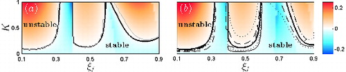The most unstable region is ξ _f < 0.2, which can also be seen from the red regions in Figure 3(a) indicating large cycle increments Γ = exp (2π(λ/ω)) − 1, i.e. large relative growth per cycle of oscillation.

Figure 3. Linear stability map in (ξ _f , K)-space, with coloured shading indicating cycle increment Γ. (a) Analysis with the DTL model: Γ and stability bound (—) from time domain analysis and stability bound (grey curve) from network analysis in the frequency domain for validation. (b) Analysis with the STL model in the time domain: Γ and stability bound for n known at ω (—), ± 1.1ω (- - -), ± 1.2ω (⋅⋅⋅). (Colour online.)

Any stability prediction relies on the quality of the models used. In the present study, the description of $\dot{q}$ stems from experimental data and is realistic. For the acoustic field, we have chosen to use a simple (less realistic) model for ease of illustration, and neglect mean flow and the area jump in the duct. For the same reason, we have chosen to use fully reflective boundary conditions on both sides of the duct, which precludes the possibility of direct comparison to experimental stability measurements. The calculations shown here can hence be improved by using a better acoustic model and experimentally determined boundary conditions, on which we further elaborate in Section 7. However, none of the assumptions made alter the validity of the proposed method and its major conclusions. In the following section, we address the shortcomings of an STL model.

6. Comparison of DTL and STL predictions

In this section, we construct and investigate an STL model for the above test case and contrast the stability predictions and flame dynamics obtained to those predicted by the DTL model. The coarse-grained slope of phase depicted in Figure 2(b) is used to estimate the time lag as τ = 1.71. The interaction index n is determined on a case-to-case basis as the gain of the FRF (see Figure 2(a) at a given frequency of oscillation ω).

6.1. Linear stability bounds

STL models yield accurate quantitative stability predictions if the gain n and absolute time lag τ are known at the dominant frequency of oscillation ω _i [8]. This is corroborated in the present study for a realistic heat source by comparing the stability bounds (full thick black lines) and cycle increments Γ (coloured shading) obtained from the DTL and STL in Figures 3(a) and 3(b), respectively. Despite slight deviations for ξ _f > 0.65, overall agreement is good. As above, the deviations stem from the truncation of the DTL for θ ⩾ 4.

As n is obtained separately for each operating point in parameter space (ξ _f , K), computing the stability map in Figure 3(b) necessitates a priori precise knowledge of ω _i at each operating point. This is of limited practical use, since in general ω _i is estimated to lie around an anticipated or expected frequency of oscillation. In Figure 3(b), we plot the stability bounds obtained from the STL model with n taken as the gain at ω _i ± 10% (- - -) and ± 20%(⋅⋅⋅ ), respectively. These deviations in frequency reflect the uncertainty in estimating ω _i . It is evident that stability is over- and under-estimated for different ξ. Therefore, changes in stability predictions do not follow a trend with uncertainity in estimating ω _i . Linear stability bounds as computed using an STL model are hence unreliable unless the exact frequency of oscillation is not known a priori.

On the other hand, computing reliable stability bounds by representing the flame dynamics in terms of a DTL does not require a priori estimation of the frequency of oscillation. The frequency of the instability is determined as part of the analysis. We hence advocate the direct use of a DTL to perform linear stability analysis in the time domain, avoiding the need to construct an STL model.

6.2. Transient flame dynamics

The question now arises of why STL models perform unreliably when used in linear stability analysis. It may be obvious from a frequency domain perspective that it is a poor assumption to set a uniform value of gain for the response of a heat source over the entire frequency spectrum. In the following, we pursue this same argument from a time domain perspective, and argue that a flame model can only produce reliable stability predictions if it is a good representation of the flame dynamics.

A full-spectrum DTL is a good representation of the flame dynamics, as it exhibits physical insight into the flame dynamics [15,16]. The shape of the DTL can be attributed to characteristic timescales, which arise from competing physical mechanisms of flame response. For the turbulent premixed swirl flame used in the present study, the overall flame response is the superposition of two responses occurring in parallel. Due to the effect of the swirler (see Figure 1), the axial acoustic wave, by which the swirl flame is excited, is partially transformed into a convective perturbation of circulation. Both the axial convective perturbation and the perturbation of circulation cause a flame response, each of which is characterised by a separate DTL (not shown here, see figure 9 of [16]). The resulting DTL depicted in Figure 2(c) is a superposition of these DTLs.

For details of the response mechanisms of turbulent premixed swirl flames deduced from DTLs, the interested reader is referred to [16]. In the following, we will only briefly summarise some features of the flame response that can be directly inferred from the experimentally measured DTL used in the present study.

The DTL subject to axial excitation exhibits a dominant peak at lag time θ = τ (see Figure 2(c)) indicative of a convectively dominated flame response (as observed for laminar premixed flames [15]). For longer flames, or for slower convective velocities by which the acoustically induced perturbations are convected along the flame surface, τ increases and the peak moves to larger lag times θ.

The DTL subject to the perturbation of circulation exhibits two peaks of equal magnitude, but opposite in sign (not shown here, see figure 9 of [16]). This can be attributed to flame roll-up and to a change in flame angle (and thus $\dot{q}$) due to a temporary increase/decrease in the swirl number caused by the impulsive excitation [21]. For higher swirl, the two humps move to smaller lag times θ due to the decrease in flame length.

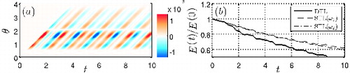
The DTL hence contains the full dynamics of the heat source with all timescales involved in the flame response (within the measured range). This is visualised in Figure 4(a), which depicts a time trace of lagged velocities weighted by the DTL, i.e. the integrand h(θ) v_f (t − θ) of the convolution yielding $\dot{q}$. The operating point is that of a stable system (ξ _f = 0.25, K = 0.18, Δ _T = 2.25), which is initialised by an equally weighted linear combination of the two most dominant thermoacoustic eigenmodes (frequencies of oscillation ω₁ = 4.11 and ω₂ = 8.62). The flame dynamics involved in the flame response as discussed in the previous paragraph is visible.

Figure 4. (a) Time trace of v_f (t − θ) weighted by the DTL. The operating point is that of a stable system, initialised at the two most dominant eigenfrequencies of oscillation, ω₁ = 4.11 and ω₂ = 8.62. The integral over θ yields $\dot{q}\left(t\right)$. Other parameters: ξ _f = 0.25, K = 0.18, Δ _T = 2.25. (b) Time trace of normalised acoustic energy E for the same case as in (a)): DTL ( − − − ), STL with n at ω₁ (− −), STL with n at ω₂ (− - − -). (Colour online.)

In contrast, the entire flame dynamics as depicted by the STL model is lumped into the parameters n and τ, where τ corresponds to only one of the humps in the DTL (see Figure 2(c)). The STL model is a weighting function fitted to one particular frequency at the operating point. The STL model reaches its limits if the system operates at a state where multiple modes interact.

The latter point becomes visible when plotting the evolution of acoustic energy E corresponding to the operating point in Figure 4(a) and obtained from the DTL model (see thick full line in Figure 4(b)). In the same plot are overlaid the evolution of energy as obtained from the STL model for which n has been determined to match the gain at the first and second eigenfrequencies, ω₁ (− −) and ω₂ (− - − -), respectively. In both cases, the evolutions diverge for t > 3. The STL model is hence incapable of representing the flame dynamics if the system does not evolve at a single frequency. If the number of eigenmodes that contribute significantly to the system state is increased further, the chance of the STL model predicting the correct transient behaviour decreases.

A slight change in n and/or τ (corresponding to n and/or τ being fitted to a different mode) hence leads to a significantly different behaviour. The same holds true for stability analysis, where the stability predictions become unreliable once the parameters n and/or τ are not known precisely.

7. Outlook

This paper outlines how to model a thermoacoustic system in the time domain using distributed time lag (DTL) response functions to incorporate the dynamics of coupled inputs (i.e. system elements that are frequency-dependent on the states). We show how to extract the DTL function from numerical/experimental frequency response data and to use it in a linear stability analysis. In addition to growth/decay rates, this approach enables physical interpretation and understanding of the mechanisms leading to the observed stability behaviour. This is possible with little computational effort by using low-order models that retain the rich dynamical behaviour of the element of interest contained in numerically/experimentally measured FRF data. For ease of illustration, the present analysis is exemplarily conducted for the DTL function of a heat source. However, the approach is definitely not limited to the modelling of combustion dynamics, and can easily be applied to other elements such as boundary conditions or damping models.

By focusing on the DTL function of a heat source, the present study highlights the shortcomings of STL models commonly employed for this element. It is shown that STL models are only adequate for stability analysis if the dominant eigenfrequencies of the entire system are known, thus leading to reliable estimates for the parameters n and τ. Knowledge of the eigenfrequencies, however, relies on the prerequisite of already having performed a stability analysis using a DTL model to represent the heat source dynamics. In contrast, a DTL model can be extracted from experimental/numerical FRF data in a straightforward manner. Hence we strongly advocate the use of DTL models in constructing low-order thermoacoustic models. In addition, DTL models inherently reflect all timescales of flame response and can be interpreted physically. By representing the full flame dynamics, they can be used for transient analysis, whereas an STL model cannot represent the system dynamics if the latter operates at a point where multiple modes interact.

In the present study, it is not possible to compare the computed stability bounds to experimentally obtained measurements, as we have chosen to use fully reflective boundary condition for ease of illustration. It is clear that simplified boundary conditions have a large impact on the stability bounds (in analogy to an oversimplified heat source model). However, as outlined in Section 2 (see Equations 1(1) $${\mathrm{d}}_t\mathbf{x}=A\mathbf{x}+\sum _{i=1}^{N_u}{B}_i{\mathbf{u}}_i,$$(1) –3(3) $$det\left[sI-A-\sum _{i=1}^{N_{\theta }}{B}_i{F}_i\left(s\right)\right]=0,$$(3) ), the concepts laid out in this paper on how to incorporate DTL functions in a time domain stability analysis equally apply to experimentally determined boundary conditions. In analogy to determining the DTL function of a heat source from FRF measurements, the same can be done from impedance measurements of a boundary condition. This matter is addressed in a related context in [22,23]. It is hence a straightforward step to model realistic thermoacoustic setups by low-order models that incorporate the rich dynamics of the system contained in multiple DTL functions.

The present study is limited to the linear regime. From the authors’ perspective, an extension to the nonlinear regime of the current approach is not straightforward. Although it is conceivable to construct an amplitude-dependent DTL function (i.e. the rational function approximation would need to be applied to amplitude-dependent describing function measurements and then be parametrised as a function of amplitude), use and implementation of such a DTL function are debatable. One of the main difficulties is the question of reference amplitude. Given a time series that contains a variety of amplitudes, it is not clear how to determine the appropriate reference amplitude, which in turn is required as an additional parameter in the amplitude-dependent DTL function. An amplitude-dependent DTL function could therefore only be used for harmonic stationary signals, and transients could not be resolved. This would deprive the method of the main benefits of a time domain approach, and thus would not represent any advantage compared to the describing function framework in the frequency domain. On the other hand, a viable possible extension of DTL functions to the nonlinear regime was proposed by Selimefendigil and Polifke [24]. They make use of nonlinear models that do not suffer from the above mentioned shortcomings.

As mentioned in Section 1, Paschereit and co-workers [5,6] have shown how to construct extremely low-order black box time domain models for duct parts and boundary conditions based on the scattering/impedance behaviour of these elements. This approach comes at the expense of the states not being physically interpretable. However, it would be possible to combine the approach of Paschereit et al.with the one outlined in the present study, so as to resolve the thermoacoustic elements whose dynamics is of interest, and to combine them with very low-order models for the elements of lesser interest. It is also conceivable to combine these two approaches with elements that are modelled by CFD, or finite-volume- and finite-element-based methods.

Acknowledgements

Thanks to J. Hoepffner and to L. Tay-Wo-Chong for their kind assistance in preparing some of the figures.

Disclosure statement

The authors have no financial interest in the results of this research project.

Additional information

Funding

The authors gratefully acknowledge financial support by the German Research Foundation DFG [project PO 710/12-1] and the Institute for Advanced Study of the Technische Universität München in the framework of a Hans Fischer Senior Fellowship for R.I. Sujith, funded by the German Excellence Initiative.

Appendix A. Discretised operators and distributions

According to Equation (5(5) $${\mathrm{d}}_t\left[\begin{array}{c}\mathbf{x}\\ {\mathbf{x}}_{\theta }\end{array}\right]=\underset{\Lambda }{\underbrace{\left[\begin{array}{cc}A& B\\ B_{\theta }& A_{\theta }\end{array}\right]}}\left[\begin{array}{c}\mathbf{x}\\ {\mathbf{x}}_{\theta }\end{array}\right].$$(5) ), the full discretised system operator Λ is given as (A1) $$\Lambda =\left[\begin{array}{cc}A& B\\ B_{\theta }& A_{\theta }\end{array}\right].$$(A1) Using the schemes as introduced in Section 5 and discretising the state vector as shown in Equation (12(12) $$\left[\begin{array}{c}\mathbf{x}\\ {\mathbf{x}}_{\theta }\end{array}\right]=\left[\begin{array}{c}{[v_1,...,v_{N_a},p_2,...,p_{N_a}-1]}^{\mathrm{T}}\\ {[v_f(t-{\theta }_1),v_f(t-{\theta }_2),...,v_f(t-{\theta }_{N_{\theta }})]}^{\mathrm{T}}\end{array}\right].$$(12) ), the discretised operators read (A2) $$\begin{array}{c}\hfill A=\left[\begin{array}{cc}{A}_{vv}& A_{vp}\\ A_{pv}& A_{pp}\end{array}\right],\in {\mathbb{R}}^{(2N_a-2)\times (2N_a-2)},\end{array}$$(A2) (A3) $$\begin{array}{cc}\hfill B_{ij}& =K\Delta \theta \left[d_i^d{h}_j^d\right],\in {\mathbb{R}}^{(2N_a-2)\times N_{\theta }},\end{array}$$(A3) (A4) $$\begin{array}{c}\hfill B_{\theta ,ij}=\frac{-1}{2\Delta \theta }\left\{\begin{array}{cc}\hfill -1& \text{for}i=1\wedge j=n_f\hfill \\ \hfill 0& \text{otherwise,}\hfill \end{array}\right.\in {\mathbb{R}}^{N_{\theta }\times (2N_a-2)},\end{array}$$(A4) (A5) $$\begin{array}{c}\hfill A_{\theta }=\frac{-1}{2\Delta \theta }\left[\begin{array}{ccc}0\hfill & 1& 0\\ -1\hfill & 0& 1\\ -1& 0& 1\\ \ddots & \ddots & \ddots \\ -1& 0& 1\\ -1& 0& 1\\ 1& -4& 3\end{array}\right],\in {\mathbb{R}}^{N_{\theta }\times N_{\theta }},\end{array}$$(A5) where n_f Δξ = ξ _f and with discrete IR function $h^d={[h_1,h_2,...,h_{N_{\theta }}]}^{\mathrm{T}}$. The discrete distributions of heat release rate d^d and of speed of sound β ^d are given as discrete normal probability and cumulative distribution functions, (A6) $$\begin{array}{c}\hfill d_i^d=\left\{\begin{array}{cc}\hfill 0& \hfill \text{for}i\le N_a\\ \hfill {\displaystyle \frac{1}{\sigma \sqrt{2\pi }}exp\left({\displaystyle -\frac{{\left({\xi }_{i-N_a+1}^d-{\xi }_f\right)}^2}{2{\sigma }^2}}\right)}& \hfill \text{for}i>N_a,\end{array}\right.\in {\mathbb{R}}^{(2N_a-2)\times 1},\end{array}$$(A6) (A7) $$\begin{array}{c}\hfill {\beta }^d=\frac{\left(\sqrt{{\Delta }_T}-1\right)}{2}\left[1+\text{erf}\left(\frac{{\xi }^d-{\xi }_f}{\sqrt{2}\sigma }\right)\right]+1,\in {\mathbb{R}}^{N_a\times 1},\end{array}$$(A7) with discretised spatial coordinate ${\xi }^d={[{\xi }_1,{\xi }_2,...,{\xi }_{N_a}]}^{\mathrm{T}}$. The standard deviation σ is chosen such that at least 99.9% of the changes in distributions occur within ξ _f ± 0.025. Δθ in Equation (A3(A3) $$\begin{array}{cc}\hfill B_{ij}& =K\Delta \theta \left[d_i^d{h}_j^d\right],\in {\mathbb{R}}^{(2N_a-2)\times N_{\theta }},\end{array}$$(A3) ) results from the numerical approximation of the convolution integral defining $\dot{q}$, (A8) $$\dot{q}={\int }_0^{4}h\left(\theta \right){\mathbf{x}}_{\theta }\mathrm{d}\theta \approx \Delta \theta \sum _{k=1}^{N_{\theta }}{h}_k^d{\mathbf{x}}_{\theta ,k}^d.$$(A8)

The submatrices in A read (A9) $$\begin{array}{c}\hfill A_{vv}=\frac{\mathrm{diag}\left[{\beta }^d\right]}{2\Delta \xi }\left[\begin{array}{ccc}-3\hfill & 4& -1\\ 0& 0& 0\\ \ddots & \ddots & \ddots \\ 0& 0& 0\\ 1& -4& 3\end{array}\right],\in {\mathbb{R}}^{N_a\times N_a},\end{array}$$(A9) (A10) $$\begin{array}{c}\hfill A_{vp}=\frac{-\mathrm{diag}\left[{\left({\beta }^d\right)}^2\right]}{2\Delta \xi }\left[\begin{array}{ccc}4\hfill & -1& 0\\ 0\hfill & 1\\ -1\hfill & 0& 1\\ -1& 0& 1\\ \ddots & \ddots & \ddots \\ -1& 0& 1\\ -1& 0& 1\\ -1& 0\\ 1& -4\end{array}\right],\in {\mathbb{R}}^{N_a\times (N_a-2)},\end{array}$$(A10) (A11) $$\begin{array}{c}\hfill A_{pv}=\frac{-1}{2\Delta \xi }\left[\begin{array}{ccc}-1\hfill & 0& 1\\ -1& 0& 1\\ \ddots & \ddots & \ddots \\ -1& 0& 1\\ -1& 0& 1\end{array}\right],\in {\mathbb{R}}^{(N_a-2)\times N_a},\end{array}$$(A11) (A12) $$\begin{array}{c}\hfill A_{pp}=\zeta \mathbf{I},\in {\mathbb{R}}^{(N_a-2)\times (N_a-2)},\end{array}$$(A12) with identity matrix $\mathbf{I}$. Also, (A13) $$\mathrm{diag}{\left[{\beta }^d\right]}_{ij}=\left\{\begin{array}{cc}\hfill {\beta }_i^d& \hfill \text{for}i=j\\ \hfill 0& \hfill \text{otherwise,}\end{array}\right.\in {\mathbb{R}}^{N_a\times N_a},$$(A13) and likewise for diag[(β ^d )²].

References

- S.R. Stow and A.P. Dowling , Low-order modelling of thermoacoustic limit cycles , in Proceedings of ASME TURBO EXPO 2004 Power for Land, Sea and Air , 14–17 June 2004, Vienna, Austria. Paper No. GT2004-54245.
- T. Sattelmayer and W. Polifke , Assessments of methods for the computation of the linear stability of combustors , Combust. Sci. Technol. 175 (2003), pp. 453–476.
- T. Sattelmayer and W. Polifke , A novel method for the computation of the linear stability of combustors , Combust. Sci. Technol. 175 (2003), pp. 477–497.
- B. Schuermans , V. Bellucci , and C. Paschereit , Thermoacoustic modeling and control of multi burner combustion systems , in Proceedings of ASME TURBO EXPO 2003 Power for Land, Sea and Air , 16–19 June 2003, Atlanta, GA. Paper No. GT2003-38688.
- C.O. Paschereit , J.P. Moeck , and M.R. Bothien , State-space modeling of thermoacoustic systems for stability analysis and time domain simulation , in Proceedings of the 13th International Congress on Sound and Vibration , 2–6 July 2006, Vienna, Austria.
- M. Bothien , J. Moeck , A. Lacarelle , and C. Paschereit , Time domain modelling and stability analysis of complex thermoacoustic systems , Proc. Inst. Mech. Engrs, Pt A: J. Power & Energy 221 (2007), pp. 657–668.
- H. Mangesius and W. Polifke , A discrete-time, state-space approach for modelling non-normal effects in thermoacoustic systems , Int. J. Spray Combust. Dynam. 3 (2011), pp. 331–350.
- M. Schmid , R. Blumenthal , M. Schulze , W. Polifke , and T. Sattelmayer , Quantitative stability analysis using real frequency response data , J. Engng – Gas Turbines & Power 135 (2013), 121601. Paper No. GTP-13-1240. Available at http://dx.doi.org/10.1115/1.4025299.
- C.S. Goh and A.S. Morgans , The influence of entropy waves on the thermoacoustic stability of a model combustor , Combust. Sci. Technol. 185 (2013), pp. 249–268.
- M. Bauerheim , J.F. Parmentier , P. Salas , F. Nicoud , and T. Poinsot , An analytical model for azimuthal thermoacoustic modes in an annular chamber fed by an annular plenum , Combust. Flame 161 (2014), pp. 1374–1389.
- M. Heckl and B. Kosztin , Analysis and control of an unstable mode in a combustor with tuneable end condition , Int. J. Spray Combust. Dynam. 5 (2013), pp. 243–272.
- G. Campa , M. Cinquepalmi , and S.M. Camporeale , Influence of nonlinear flame models on sustained thermoacoustic oscillations in gas turbine combustion chambers , in Proceedings of ASME TURBO EXPO 2013 Power for Land, Sea and Air , 3–7 June 2013, San Antonio, TX.
- A. Andreini , B. Facchini , A. Giusti , I. Vitale , and F. Turrini , Thermoacoustic analysis of a full annular lean burn aero-engine combustor , in Proceedings of ASME TURBO EXPO 2013 Power for Land, Sea and Air , 3–7 June 2013, San Antonio, TX.
- L. Magri and M.P. Juniper , A theoretical approach for passive control of thermoacoustic oscillations: Application to ducted flames , J. Engng – Gas Turbines & Power 135 (2013), 091604. Paper No. GTP-13-1197. Available at http://dx.doi.org/10.1115/1.4024957.
- R.S. Blumenthal , P. Subramanian , R.I. Sujith , and W. Polifke , Novel perspectives on the dynamics of premixed flames , Combust. Flame 160 (2013), pp. 1215–1224.
- T. Komarek and W. Polifke , Impact of swirl fluctuations on the flame response of a perfectly premixed swirl burner , J. Engng – Gas Turbines & Power 132 (2010), 061503. Available at http://dx.doi.org/10.1115/1.4000127.
- P. Subramanian , R. Sujith , and P. Wahi , Subcritical bifurcation and bistability in thermoacoustic systems , J. Fluid Mech. 715 (2013), pp. 210–238.
- B. Gustavsen and A. Semlyen , Rational approximation of frequency domain responses by vector fitting , IEEE Trans. Power Delivery 14 (1999), pp. 1052–1061.
- W. Polifke and C. Lawn , On the low-frequency limit of flame transfer functions , Combust. Flame 151 (2007), pp. 437–451.
- T. Poinsot and D. Veynante , Theoretical and Numerical Combustion , 2nd ed., R.T. Edwards, 2005.
- P. Palies , T. Schuller , D. Durox , L. Y.M. Gicquel , and S. Candel , Acoustically perturbed turbulent premixed swirling flames , Phys. Fluids 23 (2011), 037101. Available at http://dx.doi.org/10.1063/1.3553276.
- A. Huber , P. Romann , and W. Polifke , Filter-based time-domain impedance boundary conditions for CFD applications , in International Gas Turbine and Aeroengine Congress & Exposition , June 2008, Berlin, ASME GT2008-51195.
- R. Kaess , A. Huber , and W. Polifke , A time-domain impedance boundary condition for compressible turbulent flow , in 14th AIAA/CEAS Aeroacoustics Conference (29th AIAA Aeroacoustics Conference) , 2008, Vancouver, AIAA-2008-2921. Available at http://dx.doi.org/10.2514/6.2008-2921.
- F. Selimefendigil and W. Polifke , A frequency domain system model with coupled modes for limit cycle prediction of thermoacoustic systems , Int. J. Spray Combust. Dynam. 3 (2011), pp. 303–330.
- L. Tay Wo Chong, S. Bomberg , A. Ulhaq , T. Komarek , and W. Polifke , Comparative validation study on identification of premixed flame transfer function , J. Engng – Gas Turbines & Power 134 (2012), 021502. Available at http://dx.doi.org/10.1115/1.4004183.