Assessment of dynamic closure for premixed combustion large eddy simulation

Abstract

Turbulent piloted Bunsen flames of stoichiometric methane–air mixtures are computed using the large eddy simulation (LES) paradigm involving an algebraic closure for the filtered reaction rate. This closure involves the filtered scalar dissipation rate of a reaction progress variable. The model for this dissipation rate involves a parameter β_c representing the flame front curvature effects induced by turbulence, chemical reactions, molecular dissipation, and their interactions at the sub-grid level, suggesting that this parameter may vary with filter width or be a scale-dependent. Thus, it would be ideal to evaluate this parameter dynamically by LES. A procedure for this evaluation is discussed and assessed using direct numerical simulation (DNS) data and LES calculations. The probability density functions of β_c obtained from the DNS and LES calculations are very similar when the turbulent Reynolds number is sufficiently large and when the filter width normalised by the laminar flame thermal thickness is larger than unity. Results obtained using a constant (static) value for this parameter are also used for comparative evaluation. Detailed discussion presented in this paper suggests that the dynamic procedure works well and physical insights and reasonings are provided to explain the observed behaviour.

Keywords:

• dynamic closure
• SDR
• premixed flames

1. Introduction

High efficiency and low emission can be achieved simultaneously for power plants used in transport sectors, specifically gas turbines, using lean turbulent premixed combustion. A strong interplay between thermochemical and fluid dynamic processes having comparable time scales in fuel-lean combustion makes this combustion prone to local extinction potentially leading to flame blow-off. An undesirable noisy combustion can ensue from this vulnerability of lean flames. Computer simulations play an important role in identifying ways to achieve stable and smooth lean combustion and to incorporate them in the design of modern combustors. However, one needs robust and reliable combustion sub-modelling to achieve this, and the large eddy simulation (LES) paradigm may be more suited than the Reynolds averaged Navier–Stokes (RANS) approach to studying the above unsteady phenomenon.

The dynamics of large-scale turbulent eddies down to a cut-off scale are solved with models to represent the influences of unresolved small (known as sub-grid) scales in a typical LES [1,2] employing a numerical grid adequate to resolve the dynamic scales containing at least 80% of the turbulence energy [1]. This method is seen to be a higher fidelity approach compared to unsteady RANS (URANS) as expressed in classical views of LES [3–7] rather than as a degenerate form of direct numerical simulation (DNS). This implies that the LES filter width Δ, inherently linked to numerical cell volume, is usually larger than the flamelet or flame front thickness in turbulent lean premixed combustion. Thus, premixed combustion is usually a sub-grid scale (SGS) phenomenon, which must be modelled. Various SGS modelling approaches used for premixed combustion are reviewed and summarised in [2,8–10]. These approaches can be broadly categorised in two classes, namely flamelets and non-flamelets [8,9]. The flamelets, or geometrical, category includes the thickened flame [11], flame surface density or flame-wrinkling (see for example [12–18]), level-set or G equation [19,20] and laminar flamelets approaches. The non-flamelets, or statistical, category includes the transported probability density function (PDF) and conditional moment closure (CMC) methodologies. The CMC method [21] was tested for RANS simulations of premixed combustion [22,23] but has yet to be applied for LES. PDF methods have been used for the LES of premixed combustion [24,25]. Each of these categories of SGS combustion modelling has its merits and drawbacks. In this study, our interest is in the flamelet based approach involving the scalar dissipation rate of a reaction progress variable c, as described briefly below.

The instantaneous scalar dissipation rate, defined as N_c = D(∇c · ∇c) with D as the molecular diffusivity of c, is a central quantity in turbulent premixed combustion and it represents the rate of mixing of reactant and product at scales relevant for combustion. The local gradient of c and thus N_c is controlled by reaction, diffusion, convection and their interplay [26]. Recognising the fundamental importance of N_c, Bray [27,28] showed a direct relationship between the mean reaction rate and the scalar dissipation rate of c as (1) for large Damköhler numbers, where C_m is a well-known thermo-chemical parameter. The validity of this expression over a wide range of combustion conditions is recognised [29,30] and its applicability for modelling the filtered reaction rate in LES has also been demonstrated using a priori analysis of DNS data [31,32] and LES [33,34]. The over-bar in Equation (1(1) ) can be taken to signify the filtering operation in LES, and denotes Favre filtered N_c, which needs to be modelled. This quantity is written as , where is the Favre filtered progress variable and the SGS part, , is modelled as [31] (2) where with θ₅ = 0.75 and Δ⁺ = Δ/δ_th is the normalised filter width. The factor ensures that when Δ⁺ → 0 [31]. The unstrained planar laminar flame speed and its thermal thickness are denoted as s_L and δ_th, respectively. The SGS velocity is u′_Δ, which is to be modelled, and the sub-grid scale Damköhler number is with u′⁺_Δ = u′_Δ/s_L. The heat release parameter is τ = (T_b − T_u)/T_u with T_b as the adiabatic flame temperature and T_u as the reactant temperature. The other parameters signifying [35] the influences of thermochemical and turbulence processes and their interplay are K*_c = 0.79τ, and C₄ = 1.1/(1 + Ka_Δ)^0.4, and the SGS Karlovitz number is [31].

It has been reasonably established in past RANS studies [35–40] that the above parameter values are not arbitrary and various terms in Equation (2(2) ) are closely related to certain physical processes involved in the transport of scalar dissipation rate [35,41]. The terms involving (K_cs_L/δ_th) and (C₃ − τC₄ Da_Δ)(u′_Δ/Δ), respectively, arise due to fluctuating dilatation and strain rate resulting from the competing effects of turbulence and heat release. Hence they are not tuneable parameters. However, the term comes from the combined influence of flame front curvature effects induced by turbulence, chemical reaction and molecular dissipation processes, which are influenced by turbulence at the SGS level. In order to calculate using Equation (2(2) ) and the filtered reaction rate through Equation (1(1) ), one needs a model for the SGS velocity scale u′_Δ and a value for β_c. Out of many plausible models for the SGS velocity scale, a simple model based on the scale similarity of the velocity field is used here and this model is written as [1] , where C_q = 1 and is the velocity field obtained using a Gaussian test filter during LES. A detailed analysis using DNS data in [32] demonstrated further that the model in Equation (2(2) ) may not be unduly sensitive to the u′_Δ model and thus the above scale similarity model is used for this study.

Although a value of β_c ≈ 6.7 worked well for the RANS counterpart of Equation (2(2) ) [22,23,35–40], this value cannot be adopted for LES because of the difference in scales for the physics of this term involved for RANS and LES combustion modelling. For example, Dunstan et al. [31] showed that β_c = 2.4 worked well for their a priori testing of Equation (2(2) ) and a dependence on τ was shown in [32]. These subtleties suggest that a dynamic approach to obtain β_c is more suited than using a static value in LES. It is worth re-emphasising here that the other parameters in Equation (2(2) ) are not arbitrary and tuneable. Thus, the objective of this study is to propose a dynamic procedure for obtaining the scale-dependent β_c value and to test this proposition using DNS data and the LES of experimental flames.

This paper is organised as follows. The dynamic procedure to get β_c is explained in Section 2 along with a power-law model for . A priori evaluation is described in Section 3 along with the salient features of DNS data used for this evaluation. The experimental flames and their setup are described briefly in Section 4 along with numerical detail, boundary conditions, and grids used for large eddy simulation. Section 4 also discusses LES results as a posteriori evaluation of the dynamic procedure and the power-law model in comparison to experimental measurements. LES statistics obtained using a constant (static) value for β_c are also used for a comparative evaluation of the dynamic approach. The conclusions are summarised in Section 5.

2. Dynamic modelling

In general, dynamic modelling is based on the assumption that an unresolved quantity of interest or its functional dependence on key quantities is similar in neighbouring scales [1]. This scale similarity assumption for flame wrinkling and flame surface density has been proposed and used in past studies [14,17,18,42–45]. Many earlier studies [46–48] have recognised that these quantities are closely related to |∇c|. Hence, the scale similarity concepts can also be equally applied to the scalar dissipation rate (N_c) field.

Equation (2(2) ) can be written as for conciseness and a comparison of this expression to Equation (2(2) ) defines f₁. The dynamic evaluation of β_c is as follows. Firstly, one writes (3a) and (3b)

with and , by using a test filter of size . Here, the notations and imply that they must involve quantities obtained using the test filter. A Gaussian filter having as its width is used for test filtering in this paper. Subtracting Equation (3b(3b) ) from Equation (3a(3a) ) and recognising that , one can obtain an expression for β_c if β_c does not change during test filtering. Also, within the modelling framework used in this study, the volume averaged is directly proportional to the volume averaged according to Equation (1(1) ) and thus the volume averaged should be independent of Δ. This allows one to write , where the subscript v denotes volume averaging, which is local for LES. This averaging will also help to improve the numerical stability for LES.

Using both parts of Equation (3) and assuming that β_c does not change during the test filtering operation, one obtains (4) To satisfy the realisability condition of , this parameter must satisfy β_c ≥ 2/(2C_m − 1) [41]. Thus, one gets (5)

For the analyses to be discussed in a later part of this paper, the volume averaging noted above was carried out as follows. For the LES analysis, three to five neighbouring numerical grid cells in each spatial direction were used and the results were found to be insensitive to this choice in this range. For the analysis using DNS data, volume averaging was carried out using (2n)³ cells around a given grid point, where n was varied from two to six and it was found that the results did not change significantly for n > 3.

Another dynamic model explored for is based on a power-law behaviour for the filtered scalar dissipation rate. The static version of this model is studied in [31,32]. This choice was motivated by many earlier studies [12,16,42,45,49–52] attempting to model the flame wrinkling factor or the generalised flame surface density using a power law, and these quantities are closely related to as noted earlier in this section. This model for is written as [31,32] (6) where α is the exponent and η_i is the inner cut-off scale, which scales as δ_th [14,16,31,53].

Using a constant and non-zero value for α in Equation (6(6) ) does not readily satisfy the expected asymptotic behaviour of  in the limit of Δ → 0. To overcome this, a dynamic evaluation can be followed. Following a method similar to that described above for β_c, one gets (7)

One can also write Equation (6(6) ) as (8) using a different exponent α₁ to satisfy the condition that as Δ → 0. If one were to have the filtered dissipation rates from Equations (6(6) ) and (8(8) ) equal, then α₁ ≈ α for Δ/η_i ≫ 1. The dynamic procedure with Equation (8(8) ) gives (9) If one takes , then one gets α₁ ≈ α for large filter widths. Thus, it is immaterial if one uses Equation (6(6) ) or (8(8) ) in LES with sufficiently large filter widths.

It is worth noting that the validity of dynamic models in Equations (4(4) ) and (7(7) ) strongly depends on the validity of scale similarity for quantities at Δ and . Specifically, the scale similarity must hold for and for Equation (4(4) ) because ψ₂ involves these two quantities, and for for Equation (7(7) ). These observations will come in handy while interpreting the results in this paper later.

3. Analysis using direct numerical simulation

3.1. DNS data

DNS data of freely propagating statistically planar turbulent premixed flames considered in [32,54] are used for the analysis in this section. Thus, only information pertinent to this investigation is discussed briefly here and further detail such as boundary conditions, numerical schemes, thermo-chemical and thermo-physical parameters, etc., can be found in those references and in [55–58]. The relevant details are given in Table 1. The computational domain is rectangular of sizes in x-, y- and z-directions given in the table and the lengths are normalised using δ_th. This domain is discretised using 230×230×230 (345×230×230) grid points for case D1 (cases D2–D6), ensuring that there are at least 10 grid points inside δ_th. This assures that the gradients required for SDR (N_c) related analysis are resolved well. The combustion is modelled using a single irreversible reaction with Arrhenius kinetics having a Zel'dovich number of six and τ = 4.5.

Table 1 Initial values and model parameters for the DNS flames.

Case	L^+x × Ly^+ × L^+z	u′/sL	Λ/δth	Ret	Da	Ka	AT/AL	α	βc	Cm
D1	24.1×24.1×24.1	7.5	2.5	47.0	0.33	13.0	1.9	1.13	3.3	0.85
D2	36.1×24.1×24.1	5.0	1.7	22.0	0.33	8.6	1.10	0.86	4.8	0.83
D3	”	6.3	1.4	23.5	0.22	13.4	1.25	0.88	4.8	”
D4	”	7.5	2.5	47.0	0.33	13.0	1.85	1.11	4.1	”
D5	”	9.0	4.3	100	0.48	13.0	3.75	1.18	4.0	”
D6	”	11.3	3.8	110	0.33	19.5	3.80	1.26	4.0	”

Out of the 11 flames in [32,54], only six flames having unity Lewis number are considered for this study. The choice of unity Lewis number is because the reactant mixture of the experimental flames considered for this study, to be discussed in the next section, has a Lewis number close to unity. The initial root-mean-square (RMS) values of turbulent velocity fluctuations (u′) normalised by s_L, range from 5 to 11.3. The integral length scale of this turbulent field (Λ) normalised by δ_th, is also given in Table 1. These six flames have turbulent Reynolds number (Re_t) ranging from 22 to 110. Since Re_t ∼ Da²Ka² for unity Lewis number flames [59], Re_t variation for cases D2–D6 is achieved by modifying the Damköhler number, Da = (Λ/δ_th)/(u′/s_L), and the Karlovitz number, Ka = (u′/s_L)^1.5(δ_th/Λ)^0.5, independently. The values in the next three columns of Table 1 will be discussed in the next subsection. The combustion conditions of these flames are in the thin reaction zones regime of the combustion diagram [59] shown in Figure 1 and the symbols F1, F2 and F3 denote conditions of the experimental flames to be discussed in the LES section.

Figure 1. Combustion regime diagram showing DNS () and experimental (), also LES, flames, where δ = ν/S_L is the Zel'dovich flame thickness with ν being the unburned gas viscosity. The Damköhler, Da_δ, and Karlovitz, Ka_δ, numbers are defined using δ instead of δ_th.

The reaction progress variable required for this analysis is defined using a product mass fraction c = (Y_P − Y^u_P)/(Y^b_P − Y_P^u) with the superscripts b and u, respectively, denoting the burnt and unburnt mixtures. The gradients of this c field are obtained using higher order finite difference schemes consistent with those used for the DNS. These DNS data are filtered using a Gaussian filter having 0.4 ≤ Δ⁺ ≤ 2.8 for a priori analysis of the dynamic models discussed in Section 2. Typical results from this analysis are discussed next using the flames D2 and D6, because they represent extreme values of the Re_t range in Table 1.

3.2. Analysis of the DNS results

The variation of with Δ⁺ extracted from the DNS data is shown in Figure 2 for the D2 and D6 flames. A linear variation in a log–log plot implies a power-law behaviour, which is observed only for Δ⁺ > 1.5. The slope of the best fit straight line shown for these two flames gives an α-value, and its intersection with the line gives the value of the normalised inner cut-off scale, η⁺_i. The results in Figure 2 suggest that η⁺_i ≈ 1 for both flames and a similar value was observed for other flames listed in Table 1, which is consistent with the findings in [31,32]. The values of the exponent α are given in Table 1 for all the six flames and these values suggest that α ∼ Re_t^0.22. This increase is consistent with a larger extent of flame wrinkling at high Re_t, which can be substantiated from the normalised flame surface area, A_T/A_L, listed in Table 1. These data also suggest that A_T/A_L ∼ Re_t^0.77. Since these approximations are obtained using only six data points and the initial Reynolds number, one must be cautious in using them. The turbulent flame area, A_T, is evaluated using the volume-integral of |∇c|, and a similar method is used to get the laminar flame area A_L.

Figure 2. Variation of with Δ⁺ on a log–log plot along with estimates from various models for the D2 and D6 flames. The best fit lines yielding the α values listed in Table 1 are also shown.

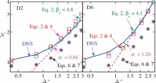
Figure 2 shows that the algebraic model in Equation (2(2) ) with (static) empirical values of β_c given in Table 1 can capture the variation of with Δ⁺ quite well in general. These values are significantly larger than the 2.7 used by Dunstan et al. [31]. This is because of larger τ values for the flames in Table 1 and this change is consistent with an empirical scaling of β_c with τ observed in [32]. A closer study of Figure 2 suggests that this static model gradually underestimates as the Δ⁺ value decreases, and this is more apparent for the higher Reynolds number case, D6, suggesting that the β_c value may also change with Δ⁺.

The values of obtained using the dynamic evaluation of β_c and α as explained in Section 2 are also compared to DNS results in Figure 2. For the lowest Reynolds number case, D2, the dynamic β_c model seems to overestimate for larger Δ⁺ values and the agreement is quite good for lower Δ⁺ values as seen in Figure 2. However, the agreement is improved uniformly for the larger Re_t case shown in this figure. The exponent of the power law, α, obtained using the best fit line is also given in the figure and the values of α for other flames are listed in Table 1. The power-law based dynamic model in Equations (6(6) ) and (7(7) ) underestimates severely as seen in Figure 2 and the level of this underestimate seems to increase with Re_t. The reason for this underestimate will become clear after studying the variation of with because the results in Figure 2 are for a volume-averaged dissipation rate and one needs to understand the local variation of .

The variations of averaged , conditional on bins of , estimated by the two dynamic models are compared to the DNS results in Figure 3 for Δ⁺ = 0.4 and 2.8. It is to be noted that these filter widths, respectively, give and 5.6 for the test filter, while the grid resolution is about 0.1δ_th. Thus, these two filter widths represent a good range such as one would expect in a typical LES of premixed flames. The global behaviour observed in Figure 2 is consistent with the local behaviour shown in Figure 3. The power-law model underestimates local conditional upon values for as seen in Figure 3 for both filter widths. The level of this underestimate is larger for D6. As noted earlier, is assumed to be scale-similar at test-filtering level with for the power-law model in Equation (7(7) ) and this assumption seems to break down for the following reason. This gradient inside the flame is larger than its value outside the flame and so must lie entirely within the flame for this assumption to hold. Thus, the dynamic power-law model will work reasonably if and this cannot be tested reliably using the current DNS data because the smallest filter width used is already close to the limit of grid resolution. The power-law based model for flame surface density and flame wrinkling factors was shown to be good in previous DNS studies [12,16,42,45,49–52]. However, the above condition for test filtering can only be satisfied in LES calculations having Δ ∼ (V_cell)^1/3 ≪ δ_th, where V_cell is the smallest LES computational cell volume. This condition will invariably dictate many tens of millions of computational cells for LES of premixed flames. Also, a single value for α is inadequate because of the multi-fractal nature of SDR [31]. Overall, the dynamic β_c based model seems a better choice than the power-law based model for large eddy simulations because the scale similarity of and the required for Equation (4(4) ) is relatively easier to satisfy and thus a relatively coarser grid can be used for this model.

Figure 3. Variation of mean values of conditional on bins of .

A careful examination of Equation (4(4) ) suggests that β_c is undefined if is zero because this parameter loses its physical meaning outside the filtered flame since the physical processes behind this parameter occur only in the flame (see Section 1 ‘Introduction’). To ensure this, a condition of is imposed while evaluating β_c using Equation (4(4) ) and the PDF of β_c is shown in Figure 4 for the D2 and D6 cases with Δ⁺ = 2.8. It is observed that this PDF does not change unduly when the upper and lower limits of are changed, respectively, to 0.9 and 0.1. The PDF shapes and the average β_c values are not very different for these two flames given that they have substantially different turbulent Reynolds numbers. The lower β_c limit is imposed by the realisability condition in Equation (5(5) ). For the cases with Δ⁺ = 0.4, the values of β_c are limited by the realisability condition and thus the PDF has a peak around this value (not shown here).

Figure 4. PDF of β_c for the D2 and D6 cases. The realisability limit, 2/(2C_m − 1), and the average value of β_c are also marked above.

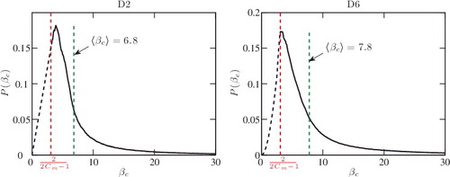
It is worth noting that the range of Re_t for these flames is small compared to the conditions in a practical combustor. However, a typical Re_t value of a laboratory scale turbulent premixed flame is of the order of 150 [60], which is not too far from 110 in Table 1. Moreover, the value of the Reynolds number for the transition to turbulence depends on the flow configuration, for example this transition Reynolds number is about 20 for a jet [61,62]. Thus, the values of Re_t given in Table 1 are not too low to disregard, or to extract meaningful and useful insights from for modelling purposes. Also, the behaviours of the filtered dissipation rate, β_c and PDFs for D2 and D6 flames having very different values of Re_t are very similar, as seen in Figures 2, 3 and 4. However, it must be mentioned that Δ⁺ > 2 will imply that the filter width is larger than the integral length scale in the case D2 and this situation is beyond a typical LES scenario.

4. Assessment using LES

4.1. Experimental flames

The piloted stoichiometric methane–air Bunsen flames of Chen et al. [63] considered in several previous studies, see for example [36,64], are chosen to conduct a posteriori analysis of the dynamic models described in Section 2. The fuel jet has a diameter of D = 12 mm and issues into quiescent air. This jet is surrounded by laminar pilot flames of a stoichiometric methane–air mixture and the pilot diameter is D_p = 68 mm. This pilot ring is water cooled and thus its burnt mixture is sub-adiabatic. The turbulence in regions with combustion is shear driven as there is no turbulence generating device in the reactant flow path. The three flames F1, F2 and F3 in [63], respectively, have bulk mean velocities of U_b = 65, 50 and 35 m/s and their jet exit Reynolds numbers based on U_b are 52,000, 40,000 and 24,000, these values having been achieved in experiments by varying only U_b. The conditions of turbulent premixed combustion in these flames shown in Figure 1 are in the thin reaction zones regime [59]. The conditions of F1, F2 and F3 are calculated using the centreline values of u′ and an integral length scale, Λ, of 2.4 mm near the nozzle exit reported in [63].

The radial variation of averaged temperature, streamwise velocity, turbulent kinetic energy, and various species mass fractions at axial locations ranging from x/D = 2.5 to 10.5 were measured and reported in [63]. These are useful for evaluating the effectiveness of the dynamic evaluation of β_c compared to its static counterpart. Furthermore, these flames were considered in many past numerical studies using RANS (see for example [36]) and LES [64] methodologies using various combustion models and thus a comparative evaluation can be made.

4.2. LES detail

The Favre filtered transport equations for conservation of mass and momentum are solved along with additional filtered equations required for combustion. The sub-grid stresses are modelled using the dynamic Smagorinsky model [1]. The test-filter size for all dynamic procedures used in this study is with the filter width computed as Δ = (V_i)^1/3, where V_i is the volume of computational cell i. The additional equations to be solved include the Favre filtered progress variable, , and the total enthalpy, , which is the sum of the sensible and chemical enthalpies of the mixture. Out of many possibilities for defining the instantaneous c, it is defined here using the fuel mass fraction Y_f as c = 1 − Y_f/Y_{f, u} so that it takes values of 0 and 1 in the unburnt and burnt mixtures, respectively. The fuel mass fraction in the unburnt mixture is denoted as Y_{f, u}. The above definition of c avoids spurious flames that would appear numerically in the mixing layer between the pilot and the coflow if it were defined using temperature T or any other species mass fraction.

The SGS scalar fluxes in and are obtained using the dynamic Schmidt number formulation [65]. The filtered reaction rate is modelled using Equation (1(1) ) and the dynamic procedure described in Section 2. To handle sub-adiabatic mixtures coming from the pilot stream, the transport equation for is included. The standard form of these equations can be found in [2]. The filtered temperature, , is obtained from the computed using , where is the specific heat capacity at constant pressure for the mixture and it depends on temperature as described in [39]. The mixture density is computed using the state equation: , where is the filtered pressure, is the Favre-filtered molecular weight of the mixture and is the universal gas constant. The values of , and are specified through a lookup table for LES as described below. This table is constructed using a planar unstrained laminar premixed flame of a stoichiometric methane–air mixture computed using the PREMIX code [66] and the GRI 3.0 mechanism with the mixture averaged diffusivity formulation. This laminar solution is then convoluted using a Gaussian filter kernel having a width equal to the cube root of the smallest computational cell volume used for the turbulent flame. This lookup table contains , and the filtered mass fractions of various species as a function of . The sensitivity of the computed results to this filter kernel width is assessed to be negligible. However, the above approach of using an unstrained laminar flame solution does not include possible effects of fluid dynamic strain on flame fronts in LES. One must be aware of this when comparing the LES statistics with measurements in Section 4.4.

A transport equation for a filtered fluid marker, , is also included to account for the influences of air entrained by the reactant jet, as had been done in [36]. These effects were assessed to be important to capture the averaged values of various species mass fractions for x ≥ 4.5D, specifically for the high Reynolds number flame F1, and thus this is included in this study. Briefly, the influence of entrained air is included using a mixing rule [36] written as , where is a generic variable representing or or or filtered mass fractions. The subscript ‘reac’ denotes that these values are taken from the lookup table for the local value, while the subscript ‘air’ denotes their values in the air stream. Further detail on this can be found in [36].

4.3. Numerical method, grid, boundary and initial conditions

The conservation equations for filtered variables along with SGS combustion modelling are solved using PRECISE-MB, which is based on finite volume methodology [67]. The spatial derivatives are discretised using a second order central differencing scheme and time advancement is by using a second order accurate scheme with a constant time step chosen to keep the CFL number smaller than 0.3 in the computational domain. Velocity–pressure coupling is achieved using the SIMPLEC algorithm [68].

A three-dimensional computational domain spanning 40D in the axial and radial directions as shown in Figure 5 is considered and it is discretised using a structured multi-block grid having non-uniform numerical cells. These cells are finer near the burner exit and grow slowly in the downstream and radial directions. A coarser grid having 22 cells inside the jet diameter, D, and about 4 cells within the turbulence integral length scale, measured to be about Λ = 2.4 mm [63] near the exit, gives a total of about 1.5 million cells for the computational volume of π(40D)³/4. This grid has 404 cells in the streamwise direction along the centreline. Increasing the cell count to 32 for D and 6 for Λ, keeping other grid parameters almost the same, yields about 4.2 million cells in total. These two grids are used to assess the grid sensitivity of the LES results. The coarse grid having 1.5M cells satisfies the 80% turbulent energy criterion of Pope [1] and has Δ⁺_min ≈ 1.3. The fine grid of 4.2M has Δ⁺_min ≈ 0.8.

Figure 5. A schematic of the computational setup for the piloted stoichiometric methane–air Bunsen flames of Chen et al. [63].

The jet exit velocity is specified using the radial profile reported in [63]. No fluctuation in the jet exit velocity is specified since turbulence in the reacting region is shear generated. Analyses of cold flows, to be discussed later in this section, show that the correct turbulence is recovered after a few diameters from the jet exit for the numerical grid and other simulation parameters used in this study. A uniform velocity of 1.5 m/s is specified for the pilot stream on the basis of the total volumetric flow rate obtained from the experimental data. A small velocity of 0.2 m/s is assigned to the coflowing air to mimic air entrainment. The pilot stream is specified to have a uniform temperature of 1950 K as in a previous RANS [36] analysis. This temperature is not reported in the experimental study [63] and thus this boundary condition has some uncertainty. However, many earlier numerical investigations of these flames suggested that this uncertainty influences only the temperature field close to the jet exit (x ≤ 3D), which is also confirmed in this study by changing the pilot temperature over a range of about 200 K in a preliminary analysis. The filtered progress variable is specified to be zero in the jet exit and one for the pilot and coflowing streams. The lateral boundaries are specified to be slip walls and the outlet is set to have zero gradients in the streamwise direction for all the variables.

The large eddy simulations are run using 96 cores (2.60 GHz Intel Sandy Bridge E5-2670 processors) on Darwin cluster at Cambridge University for about 0.15 to 0.25 seconds of real flow time. Out of these total durations, the period of data collection for averaging and analysis corresponds to about 32 flow-through time for F1, 26 for F2 and 22 for F3, where the flow-through time is defined using the computational domain length and the respective bulk-mean velocity, U_b, at the jet exit. These sampling times are very much larger than those used typically in past studies. These simulations took about a day for 1.5M and two days for 4.2M grids on a wall clock using the above computational cluster when β_c is treated to be a static value. These computational times are observed to increase by about 7% when the dynamic β_c model is used. This small increase is because of the relatively small grid sizes (1.5M and 4.2M) used here.

4.4. LES results and discussion

The LES results are time averaged first over the data sampling period and then averaged in the azimuthal direction in order to get the radial variation of mean quantities at various axial positions as reported in the experimental study [63]. This averaging procedure is denoted using ⟨·⟩ in the following discussion. Although all three flames, F1, F2 and F3, are simulated using both the static and dynamic models described in Section 2, typical behaviours of these models are elucidated using the flames F1 and F3. Also, the numerical grid, SGS stress and scalar flux closures are kept the same in order to compare the static and dynamic procedures for β_c.

Figure 6 shows a typical comparison of the radial variation of ⟨U⟩/U_b and ⟨k⟩/k_o with respective measurements for five axial positions, where U_b = 50 m/s and k₀ = 10.8 m²/s² for the flame F2. The turbulent kinetic energy (TKE), k, is obtained as k = 0.5∑⟨u_iu_i⟩ + 1.5⟨u′²_Δ⟩, where . The comparison for ⟨U⟩ shown in Figure 6 suggests that the boundary conditions, numerical grids and methods used in this study are good for modelling these flows. Also, the differences between the 1.5M and 4.2M grid results are negligibly small for both and normalised ⟨k⟩. Some differences are observed for ⟨k⟩ in regions of r ≤ 0.55D, and these decrease as one moves in the downstream direction. As seen in Figure 6, the turbulence levels represented by ⟨k⟩ in regions of combustion, which would be r > 0.6D as one shall see later, are captured quite well despite no turbulence having been specified for the jet fluid. However, specifying some inlet turbulence comparable to the measured values did improve the comparison of ⟨k⟩ for x/D = 2.5 but no significant changes were observed for other downstream locations because the turbulence is dominated by the shear generation mechanism in this flow configuration. Thus, ignoring a small level of inlet turbulence is acceptable. The 80% criterion of Pope [1] for TKE is satisfied by the 1.5M grid used here. Thus, it is clear that this grid is adequate to capture the flow dynamics in the jets simulated here and hence this grid is used for flame calculations to be discussed next. Nevertheless, the 4.2M grid is also used for further testing and verification for reacting cases, as and when required.

Figure 6. Comparison of measured [63] (symbols) and computed (lines) normalised mean axial velocity and turbulent kinetic energy in cold flow of flame F2. The radial variations are shown for five axial locations and two numerical grids, 1.5M (solid line) and 4.2M (dotted line).

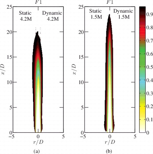
Figure 7 shows the spatial variation of the mean progress variable field, , in the flame F1 obtained using both static and dynamic approaches for β_c and the results are shown for both the 1.5M and the 4.2M grid. The reason for this will become clear in Section 4.5. However, a close study of this figure suggests that the flame brush is thinner for the dynamic β_c model leading to a slightly shorter flame brush as seen in Figure 7. If one compares the results of the 4.2M and 1.5M grids then the flame brush computed using the 1.5M grid is about 2D to 3D longer compared to that obtained using 4.2M grid. This is for the following reason. The dynamic β_c model overestimates the filtered dissipation rate, and thus also the filtered reaction rate, when Δ⁺ is less than one, as observed in Figure 3 using the DNS data (see the result for the D6 flame with Δ⁺ = 0.4). As noted earlier, the 4.2M case has Δ⁺ smaller than unity in regions of intense reaction, which satisfies the above condition. Thus, the increased filtered reaction rate leads to a shorter flame for the 4.2M case as seen in Figure 7. However, using a static value for β_c underestimates the local and volume averaged dissipation rate for Δ⁺ < 1 (see Figure 2).

Figure 7. The spatial variation of mean progress variable field for flame F1 obtained using static and dynamic approaches for β_c. This comparison is shown for both the 1.5M and 4.2M grids.

The radial variations of averaged axial velocity, normalised using the respective bulk mean velocity at the jet exit, computed using the dynamic and static β_c values are compared to the experimental measurements [63] in Figure 8 for the F1 and F3 flames. The results from both the 1.5M and 4.2M cases are shown for a few axial locations investigated in the experimental study of Chen et al. [63]. It is hard to distinguish the various curves for the flame F1, having the largest turbulent Reynolds number, suggesting that the computed averaged axial velocity is insensitive to the choice of β_c modelling and the numerical grid. The insensitivity to the numerical grid can also be seen for the flame F3, which suggests that the chosen grids are good. A small difference is seen in ⟨U⟩/U_b for the flame F3 as in Figure 8 and this difference grows to about 20% at an axial location of x = 8.5D and a radial position of about 0.8D. This is because the value of β_c obtained dynamically is smaller than the static value used for these locations. As one shall see later, the combustion is almost completed before this radial position for this axial location and the difference in β_c values is because of some small differences in the gradients of . The variations and comparisons shown in Figure 8 are typical of many earlier numerical studies of these piloted Bunsen flames and thus the statistics shown here are acceptable.

Figure 8. Comparison of measured [63] (symbols) and computed (lines) radial variation of normalised axial velocity, ⟨U⟩/U_b, obtained using dynamic (dark curves) and static (light curves, green curves in online version)β_c models for flames F1 and F3. The results are shown for the 1.5M (solid lines) and 4.2M (dotted) grids.

The computed averaged TKE normalised using its centreline value, k₀, near the jet exit is compared to the measurements for a few axial locations in F1 and F3 flames in Figure 9. The values of k₀, 12.7 for F1 and 3.82 m²/s² for F3, reported in [63] are used for this study. The comparisons seen in this figure are typical of many earlier studies. However, the agreement with the experimental data can be improved further than shown here by using finer grids as has been demonstrated in [64], but we restrict ourselves to relatively smaller grids to study the efficacies of dynamic β_c modelling for filtered reaction rate closure. This is because the closure in Equation (1(1) ) works well when Δ⁺ ≫ 1 [31,32] and Δ⁺ is already smaller than unity for the 4.2M grid used here. Thus, refining the numerical grid further will yield Δ⁺ ≪ 1, which would invalidate the closure in Equation (1(1) ) as noted in [31–33]. Moreover, refining the grid further would not be in line with a broader objective of this study as noted in Section 1 ‘Introduction’.

Figure 9. Comparison of measured [63] (symbols) and computed (lines) radial variation of normalised mean turbulent kinetic energy, ⟨k⟩/k₀. The legend is as in Figure 8.

A close study of the results in Figure 9 suggests that the peak values of ⟨k⟩/k₀ obtained using both static and dynamic β_c are similar to one another and also to measured values. However, the radial location of this peak value obtained using the dynamic approach agree quite well with the measurement and the agreement, in general, at downstream positions is improved when the 4.2M grid is used for flame F1 as one would expect. If one plots the radial variation of the u′_Δ contribution to ⟨k⟩ for downstream positions (not shown here) then the shift in radial location of peak ⟨k⟩ can be seen distinctly when the dynamic β_c model is used. This shift would be reflected in the flame related quantities, especially at downstream locations, through the influence of u′_Δ on the modelling of the filtered scalar dissipation rate and reaction rate.

The radial variations of averaged fuel mass fraction and normalised temperature are compared with experimental results [63] in Figures 10 and 11, respectively. These results are shown for both the F1 and F3 flames. The variation of averaged fuel mass fraction obtained using the power-law based model is also shown in Figure 10 for both flames computed using the 4.2M grid. The variation of averaged fuel mass fraction computed using this model suggests that this model is not representing flame behaviour, but rather convective–diffusive scalar behaviour. This is because the scale similarity for the gradient of does not hold even on the finest, 4.2M, grid used in this study because Δ⁺_min is of order unity. This gradient is non-zero only inside the resolved flame suggesting that there must be at least three points within δ_th for this scale similarity to hold implying that the test filter width must be smaller than 0.5δ_th. This gives a severe underestimate of α and thus leading to the overestimate of the averaged fuel mass fraction values seen in Figure 10. The above grid requirement condition demands that the current grid should be refined at least by a factor of 27 (3 in each direction) for the power-law based model to work reasonably in large eddy simulations. This gives many tens of millions of grid cells, increasing the computational cost enormously, perhaps to impractical proportions for industry applications. The dynamic evaluation of β_c in Equation (4(4) ) involves scale similarity for and , and thus this assumption of scale similarity can be met with a relatively coarser grid. Also, the above reasoning and the discussion in Section 3.2 require that Δ⁺ ≪ 1 for the power-law model to work reasonably well. This condition contradicts the requirement Δ⁺ > 1 for Equation (1(1) ) [31,32]. For these reasons, the power-law based model is not considered further in this study.

Figure 10. Comparison of measured [63] (symbols) and computed (lines) radial variation of mean fuel mass fraction. The legend is as in Figure 8. The dash–dotted line is for the power-law based model in Equations (6(6) ) and (7(7) ) for the 4.2M grid.

Figure 11. Measured [63] (symbols) and computed (lines) radial variations of normalised mean temperature are compared above. The legend is as in Figure 8.

There is some improvement in the computed statistics for the fuel mass fraction when the dynamic β_c approach is used and this improvement is apparent for the fine grid used in this study, especially in the region of strong gradients of fuel mass fraction at downstream locations, specifically x > 4.5D for the F1 flame. The reason for this is related to the prediction of u′_Δ and thus ⟨k⟩ discussed in Figure 9. The large difference in the statistics obtained using the dynamic model on 1.5M and 4.2M grids observed for r ≤ 0.3D, especially at the downstream locations for flame F1, cannot be commented upon because of the absence of experimental data in these radial positions. Overall, results for the CH₄ mass fraction are good and comparable with previous studies [36,64] despite the relatively small grids used here.

The variations of averaged normalised temperature shown in Figure 11 are consistent with the results for the fuel mass fraction. The dynamic evaluation of β_c seems to overestimate the fuel consumption rate compared to the static case leading to an overestimate of peak temperature. The level of this overestimate decreases as one moves downstream, implying that the performance of the dynamic approach improves for both flames F1 and F3. The large overestimate of mean temperature near the jet exit results from uncertainties in pilot stream temperature as noted in earlier studies [36,64]. However, the averaged temperature computed using the current sub-grid reaction rate closure is improved and some additional improvement from the dynamic approach is observed for downstream positions as seen in Figure 11.

The radial variations of averaged mass fractions of various scalars are shown in Figures 12, 13, 14, 15, 16 and 17. The effects of entrained air is included in the computations of these species mass fraction values as described in Section 4.2. This effect is responsible for the increasing values of oxygen mass fraction for r > 0.8D in Figure 12. The influence of dynamic evaluation of β_c on these various scalar mass fractions is found to be consistent with observations noted for averaged fuel mass fraction and temperature shown in Figures 10 and 11. The mass fractions of H₂O and H are well estimated by the method used in this study. The mass fraction of CO₂ is underestimated and the level of this underestimate is larger for the flame F1. There is a substantial overestimate in the mass fractions of CO and OH for both static and dynamic evaluation procedures for β_c. The computed increasing trend of OH mass fraction with r is improved when β_c is evaluated dynamically for the flame F1 at downstream positions as seen in Figure 15. The large overestimate of CO mass fractions seen here is consistent with many past studies.As noted earlier, the difference in various statistics obtained using the dynamic and static evaluation of β_c is observed to be small for the following reason. The static value of this parameter is obtained for these two flames empirically by conducting several simulations until an overall satisfactory behaviour is noted. The dynamic procedure described here avoids this empirical testing and the average value of β_c obtained in this procedure is comparable to the static value as one shall see next.

Figure 12. Comparison of measured [63] (symbols) and computed (lines) mean O₂ mass fractions. The legend is as in Figure 8.

Figure 13. Comparison of measured [63] (symbols) and computed (lines) mean H₂O mass fractions. The legend is as in Figure 8.

Figure 14. Comparison of measured [63] (symbols) and computed (lines) mean CO₂ mass fractions. The legend is as in Figure 8.

Figure 15. Comparison of measured [63] (symbols) and computed (lines) mean OH mass fractions. The legend is as in Figure 8.

Figure 16. Comparison of measured [63] (symbols) and computed (lines) mean H₂ mass fractions. The legend is as in Figure 8.

Figure 17. Comparison of measured [63] (symbols) and computed (lines) mean CO mass fractions. The legend is as in Figure 8.

4.5. Discussion

The PDF of β_c obtained by post-processing the LES data is shown in Figure 18 for both flames F1 and F3. This PDF is constructed using β_c values collected from the computational domain by imposing the limits and . These limits are used to avoid regions with very low reaction rates so that the values of β_c used for this PDF are physically meaningful. The contours of log β_c values obtained using Equation (4(4) ) and the above conditions are shown (as colour maps in the online version) in the insets of Figure 18. These contours are shown in the mid-plane for an arbitrarily chosen time and this variation is similar for other times. The flame brush is marked using the contours of and 0.95 and it is observed that the β_c contours mark the flame brush quite well suggesting that the conditions used to construct the PDF are meaningful. The logarithmic value is used to show clearly that the β_c variation is spatially intermittent.

Figure 18. The PDF of β_c obtained from LES of flames (a) F1 and (b) F3 using the 1.5M grid. The average value and the lower limit imposed by Equation (5(5) ) are also shown.

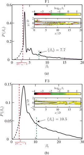
The lower limit of β_c = 3.03, for C_m = 0.83, is imposed by the realisability condition in Equation (5(5) ). The upper limit for F3 is nearly twice that for F1 and the PDF has a long tail for large β_c values for both of these flames. These PDFs are similar to those shown in Figure 4 for the DNS flames. It is worth noting that the mean values ⟨β_c⟩ given for the flames F1 and D6 are almost the same because the Damköhler and turbulent Reynolds numbers are similar for these two flames. This value of ⟨β_c⟩ ≃ 7.7 is very close to the static value of β_c = 7.5, obtained empirically as noted earlier, used for the flame F1 and thus it not surprising to observe small differences, as noted above, in various statistics obtained using the static and dynamic evaluations of β_c. The value of ⟨β_c⟩ = 10.5 given in Figure 18 for the flame F3 is larger than for F1 because of higher Da and lower Re_t values for F3, and this value is about 40% larger than the static value used for the F3 flame. This good match in the β_c values for the static and dynamic procedure for flame F1 is not coincidental. The dynamic procedure described here eliminates this empiricism while retaining the accuracy with a small increase in the computational cost. A close match in ⟨β_c⟩ values for F1 and D6 flames is also not coincidental because these two flames have similar combustion conditions as shown in Figure 1 and thus the physical processes signified by the β_c parameter are very similar in these two flames.

The efficacy of the combustion modelling approach discussed in this paper is tested further by calculating the thicknesses of the simulated flame brushes and comparing them with measured values. The results are shown in Figure 19 for both flames F1 and F3. The flame brush thickness at a given axial location is calculated as in the experimental study [63]. Thus one can recompute this thickness using the measured radial variation of normalised temperature, , shown in Figure 11. The flame brush thicknesses computed thus are compared to the values reported by Chen et al. [63] in the top row of Figure 19 for both flames. The thickness computed using normalised averaged temperature is shown as diamonds and the square symbol denoting δ_{t, Y} was obtained using the variation shown in Figure 10. The values of δ_t and δ_{t, Y} are expected to be the same for adiabatic unity Lewis number flames and a reasonable comparison is observed for the flame F3, except for the most upstream measurement location of x = 2.5D. These flame brush thicknesses compare well with those reported in [63] for this flame. For the flame F1, the differences are observed to be large and also the δ_t values recomputed here using the experimental data does not seem to agree with those reported in [63]. The difference between δ_t and δ_{t, Y} comes from the enhanced non-adiabaticity resulting from increased air entrainment in the flame F1 because of its large Reynolds number. These differences among the experimental results must be kept in mind while comparing the flame brush thicknesses computed in LES. This comparison is shown in the bottom row of Figure 19. For the flame F3, the comparison shown here is reasonable. The reaction rates are underestimated for the 4.2M grid because the combustion closure is at its limit when Δ⁺ < 1 leading to thicker flame brushes for both the F1 and F3 flames. In other words, the closure in Equation (1(1) ) is strictly valid for Δ⁺ substantially larger than unity as explained in  [31–33]. For the 1.5M grid case, the values of δ_t obtained using the static β_c model agrees very well with the measured values for the flame F3 as shown in Figure 19. The thicker flame brush for the 4.2M grid case is because the combustion closure is at its limit for this grid, as noted a few times earlier. Although the difference between the measured and computed δ_t values seems large in Figure 19, the actual difference is about 2 mm while the maximum difference observed for the comparisons shown in the top row of this figure is about 4 mm. Thus, whether the difference of about 2 mm observed between computed and measured values of δ_t is ‘big’ or ‘small’ is an open question. In our view, the comparison shown here is satisfactory and the variations of δ_t with x shown here are consistent with the results discussed earlier and also with many past numerical studies of these flames (see for example [36]).

Figure 19. The measured [63] () and recomputed, using measured versus r, values of δ_t for averaged temperature () and fuel mass fraction (□) are compared in the top row. The bottom row compares the measured and LES flame brush thicknesses for various cases.

5. Conclusions

A simple algebraic closure for filtered reaction rate is investigated in this study using static and dynamic evaluations of a model parameter involved in this closure. This reaction rate closure involves the filtered scalar dissipation rate of a reaction progress variable for premixed combustion. The particular model parameter, β_c, chosen for dynamic evaluation is related to the physics of flame front curvature effects induced by turbulence, chemical reactions, molecular dissipation, and their interactions at sub-grid level. This parameter was also shown to depend on the heat release parameter, the turbulent Reynolds number in earlier studies [32], and possibly also on filter width because of the influence of the above physical processes. Thus, the dynamic evaluation of this parameter is ideal and a dynamic procedure is discussed in this paper. The stoichiometric methane–air mixture used for the piloted Bunsen flames of Chen et al. [63] has unity Lewis number. A power-law based model is also considered for the filtered scalar dissipation rate.

A priori assessment of these models is presented briefly for the sake of completeness, and the focus of this study is on the assessment of the dynamic β_c model using LES. The LES employed 1.5M and 4.2M grids for this investigation. The various statistics, specifically the averaged fuel mass fraction variation in the radial direction at a number of axial positions, showed that the power-law based model is unable to see a flame on these two numerical grids because the scale similarity of the progress variable gradient does not hold on these two grids. For this scale similarity to hold, one needs a very fine grid (nearly two orders of magnitude larger than is used here, in terms of total size) which is impractical. Also, this scale similarity power-law based model will not work in conjunction with the algebraic closure in Equation (1(1) ). However, the scale similarity of SGS velocity and filtered progress variable, , required for the dynamic evaluation of β_c is easy to satisfy on a relatively smaller grid. The various statistics such as averaged velocity, temperature, mass fractions of different scalars, etc., obtained from LES compare well with the measured values of these quantities. LES results obtained using empirically determined (static) values of β_c are used to assess the viability of the dynamic procedure. The difference in various statistics is found to be small because the empirically determined β_c values for the three Bunsen flames are similar to the averaged value of β_c obtained in the dynamic evaluation, which is verified by analysing the PDF of β_c. The evolution of flame brush thickness with axial distance computed from LES results also compares quite well with measured values. The algebraic closure used in this study inherently assumes high Damköhler number combustion and it is of interest to extend this approach to include local finite rate chemistry effects. This can be achieved using unstrained and strained flamelets to approximate filtered flames and this will be explored in a future study.

Disclosure statement

No potential conflict of interest was reported by the authors.

Additional information

Funding

The authors express their gratitude to EPSRC, Siemens and Rolls-Royce for their support. This work is funded by EPSRC [grant number EP/I027556/1].

Notes

1. One could also have used a tabulated reaction rate instead of Equation (1(1) ), but this is not used here so as to keep the focus on the dynamic evaluation of β_c. However, remarks are made on this point when discussing the results.

2. When the tabulated reaction rate is used instead of Equation (1(1) ), the computed flow statistics and major species mass fractions differ by a very small amount in comparison to the results shown here. However, the minor species mass fractions are improved as one would expect. These results are not shown here as they are not required to address the main objective of this paper, which is the dynamic evaluation of β_c and its efficacies.

References

- S.B. Pope, Turbulent Flows, Cambridge University Press, Cambridge, UK, 2000.
- T.J. Poinsot and D. Veynante, Theoretical and Numerical Combustion, Edwards, Philadelphia, PA, , 2005.
- J. Smagorinsky, general circulation experiments with the primitive equations I. The basic experiment, Mon. Weather Rev. 91 (1963), pp. 99–164.
- D.K. Lilly, On the application of the eddy viscosity concept in the inertial sub-range of turbulence, Tech. Rep. 123, University Corporation for Atmospheric Research (NCAR), Boulder, CO, 1966.
- D.K. Lilly, The representation of small-scale turbulence in numerical simulation experiments, in Proceedings of the IBM Scientific Computing Symposium on Environmental Sciences, Yorktown Heights, NY, 1966, H.H. Goldstine, ed., IBM, 1967, pp. 195–210 ( IBM 320-1951-0).
- J.W. Deardorff, Three-dimensional numerical study of the height and mean structure of a heated planetary boundary layer, Boundary-Layer Meteorol. 7 (1974), pp. 81–106.
- U. Schumann, Subgrid scale model for finite difference simulations of turbulent flows in plane channels and annuli, J. Comput. Phys. 18 (1975), pp. 374–404.
- L.Y.M. Gicquel, G. Staffelbach, and T. Poinsot, Large eddy simulations of gaseous flames in gas turbine combustion chambers, Prog. Energy Combust. Sci. 38 (2012), pp. 782–817.
- N. Swaminathan and K.N.C. Bray, Fundamentals and challenges, in Turbulent Premixed Flames, N. Swaminathan and K.N.C. Bray, eds., Cambridge University Press, Cambridge, UK, 2011, pp. 1–40.
- R.S. Cant, RANS and LES modelling of turbulent combustion, in Turbulent combustion modelling: Advances, new trends and perspectives, T. Echekki and E. Mastorakos, eds., Springer, Heidelberg, 2011, pp. 63–87.
- O. Colin, F. Ducros, D. Veynante, and T.J. Poinsot, A thickened flame model for large eddy simulations of turbulent premixed combustion, Phys. Fluids 12 (2000), pp. 1843–1863.
- M. Boger, D. Veynante, H. Boughanem, and A. Trouvé, Direct numerical simulation analysis of flame surface density concept for large eddy simulation of turbulent premixed combustion, Proc. Combust. Inst. 27 (1998), pp. 917–925.
- E.R. Hawkes and R.S. Cant, Implications of a flame surface density approach to large eddy simulation of premixed turbulent combustion, Combust. Flame 126 (2001), pp. 1617–1629.
- R. Knikker, D. Veynante, and C. Meneveau, A dynamic flame surface density model for large eddy simulations of turbulent premixed combustion, Phys. Fluids 16 (2004), pp. L91–L94.
- N. Chakraborty and R.S. Cant, A priori analysis of the curvature and propagation terms of the flame surface density transport equation for large eddy simulation, Phys. Fluids 19 (2007), p. 105101.
- N. Chakraborty and M. Klein, A priori direct numerical simulation assessment of algebraic flame surface density models for turbulent premixed flames in the context of large eddy simulation, Phys. Fluids 20 (2008), Article ID 085108. Available at http://dx.doi.org/10.1063/1.2969474.
- S.R. Gubba, S.S. Ibrahim, and W. Malalasekera, Dynamic flame surface density modelling of flame deflagration in vented explosion, Combust. Explos. Shock Waves 48 (2012), pp. 393–405.
- G. Wang, M. Boileau, D. Veynante, and K. Truffin, Large eddy simulation of a growing turbulent premixed flame kernel using a dynamic flame surface density model, Combust. Flame 159 (2012), pp. 2742–2754.
- H. Pitsch, A consistent level set formulation for large-eddy simulation of premixed turbulent combustion, Combust. Flame 143 (2005), pp. 587–598.
- V. Moureau, B. Fiorina, and H. Pitsch, A level set formulation for premixed combustion LES considering the turbulent flame structure, Combust. Flame 156 (2008), pp. 801–812.
- A.Y. Klimenko and R.W. Bilger, Conditional moment closure for turbulent combustion, Prog. Energy Combust. Sci. 25 (1999), pp. 595–687.
- S. Amzin, N. Swaminathan, J.W. Rogerson, and J.H. Kent, Conditional moment closure for turbulent premixed flames, Combust. Sci. Technol. 184 (2012), pp. 1743–1767.
- S. Amzin and N. Swaminathan, Computations of turbulent lean premixed combustion using CMC, Combust. Theory Model. 17 (2013), pp. 1125–1153.
- D.H. Rowinski and S.B. Pope, Computational study of lean premixed turbulent flames using RANSPDF and LESPDF methods, Combust. Theory Model. 17 (2013), pp. 610–656.
- G. Bulat, W.P. Jones, and A.J. Marquis, NO and CO formation in an industrial gas-turbine combustion chamber using LES with the Eulerian sub-grid PDF method, Combust. Flame 161 (2014), pp. 1804–1825.
- N. Swaminathan and K.N.C. Bray,, Turbulent Premixed Flames, Cambridge University Press, Cambridge, UK,, 2011.
- K.N.C. Bray, The interaction between turbulence and combustion, Proc. Combust. Inst. 17 (1979), pp. 223–233.
- K.N.C. Bray, Turbulent flows with premixed reactants, in Turbulent Reacting Flows, P.A. Libby and F.A. Williams, eds., Springer-Verlag, New York, 1980, pp. 115–183.
- N. Chakraborty and N. Swaminathan, Effects of Lewis number on scalar variance transport in premixed flames, Flow Turb. Combust. 87 (2011), pp. 261–292.
- N. Chakraborty and R.S. Cant, Effects of Lewis number on flame surface density transport in turbulent premixed combustion, Combust. Flame 158 (2011), pp. 1768–1787.
- T. Dunstan, Y. Minamoto, N. Chakraborty, and N. Swaminathan, Scalar dissipation rate modelling for large eddy simulation of turbulent premixed flames, Proc. Combust. Inst. 34 (2013), pp. 1193–1201.
- Y. Gao, N. Chakraborty, and N. Swaminathan, Algebraic closure of scalar dissipation rate for large eddy simulations of turbulent premixed combustion, Combust. Sci. Technol. 186 (2014), pp. 1309–1337.
- T. Ma, Y. Gao, A.M. Kempf, and N. Chakraborty, Validation and implementation of algebraic LES modelling of scalar dissipation rate for reaction rate closure in turbulent premixed combustion, Combust. Flame 161 (2014), pp. 3134–3153.
- D. Butz, Y. Gao, A.M. Kempf, and N. Chakraborty, Large eddy simulations of a turbulent premixed swirl flame using an algebraic scalar dissipation rate closure, Combust. Flame 162 (2015), pp. 3180–3196. Available at http://dx.doi.org/10.1016/j.combustflame.2015.05.003.
- H. Kolla, J.W. Rogerson, N. Chakraborty, and N. Swaminathan, Scalar dissipation rate modeling and its validation, Combust. Sci. Technol. 181 (2009), pp. 518–535.
- H. Kolla and N. Swaminathan, Strained flamelets for turbulent premixed flames II: Laboratory flame results, Combust. Flame 157 (2010), pp. 1274–1289.
- N. Swaminathan, G. Xu, A.P. Dowling, and R. Balachandran, Heat release rate correlation and combustion noise in premixed flames, J. Fluid Mech. 681 (2012), pp. 80–115.
- I. Ahmed and N. Swaminathan, Simulation of spherically expanding turbulent premixed flames, Combust. Sci. Technol. 185 (2013), pp. 1509–1540.
- S. Ruan, N. Swaminathan, and O. Darbyshire, Modelling of turbulent lifted jet flames using flamelets: A priori assessment and a posteriori validation, Combust. Theory Model. 18 (2014), pp. 295–329.
- I. Ahmed and N. Swaminathan, Simulation of turbulent explosion of hydrogen–air mixtures, Int. J. Hydr. Energy 39 (2014), pp. 80–115.
- N. Chakraborty, J.W. Rogerson, and N. Swaminathan, A priori assessment of closures for scalar dissipation rate transport in turbulent premixed flames using direct numerical simulation, Phys. Fluids 20 (2008), Article ID 045106. Available at http://dx.doi.org/10.1063/1.2903846.
- F. Charlette, C. Meneveau, and D. Veynante, A power-law flame wrinkling model for LES of premixed turbulent combustion. Part II: Dynamic formulation, Combust. Flame 131 (2002), pp. 181–197.
- H. Pitsch, Large-eddy simulation of turbulent combustion, Annu. Rev. Fluid Mech. 38 (2006), pp. 453–482.
- E. Knudsen and H. Pitsch, A dynamic model for the turbulent burning velocity for large eddy simulation of premixed combustion, Combust. Flame 154 (2008), pp. 740–760.
- R. Knikker, D. Veynante, and C. Meneveau, A priori testing of a similarity model for large eddy simulations of turbulent premixed combustion, Proc. Combust. Inst. 29 (2002), pp. 2105–2111.
- R. Borghi, Turbulent premixed combustion: Further discussions on the scales of fluctuations, Combust. Flame 80 (1990), pp. 304–312.
- S. Pope, Computations of turbulent combustion: Progress and challenges, Proc. Combust. Inst. 23 (1990), pp. 591–612.
- D. Veynante and L. Vervisch, Turbulent combustion modeling, Prog. Energy Combust. Sci. 28 (2002), pp. 193–266.
- F. Charlette, C. Meneveau, and D. Veynante, A power-law flame wrinkling model for LES of premixed turbulent combustion. Part I: Nondynamic formulation and initial tests, Combust. Flame 131 (2002), pp. 159–180.
- E.R. Hawkes, O. Chatakonda, H. Kolla, A.R. Kerstein, and J.H. Chen, A petascale direct numerical simulation study of the modelling of flame wrinkling for large-eddy simulations in intense turbulence, Combust. Flame 159 (2012), pp. 2690–2703.
- O. Chatakonda, E.R. Hawkes, A.J. Aspden, A.R. Kerstein, H. Kolla, and J.H. Chen, On the fractal characteristics of low Damköhler number flames, Combust. Flame 16 (2013), pp. 2422–2433.
- I. Yoshikawa, Y. Shim, Y. Nada, M. Tanahashi, and T. Miyauchi, A dynamic SGS combustion model based on fractal characteristics of turbulent premixed flames, Proc. Combust. Inst. 34 (2013), pp. 1373–1381.
- W. Roberts, J. Driscoll, M. Drake, and L. Goss, Images of the quenching of a flame by a vortex – To quantify regimes of turbulent combustion, Combust. Flame 94 (1993), pp. 58–69.
- Y. Gao, N. Chakraborty, and N. Swaminathan, Scalar dissipation rate transport in the context of LES for turbulent premixed flames with non-unity Lewis number, Flow Turbul. Combust. 93 (2014), pp. 461–486.
- N. Chakraborty, G. Hartung, M. Katragadda, and C. Kaminsky, Comparison of 2D and 3D density-weighted displacement speed statistics and implications for laser based measurements of flame displacement speed using direct numerical simulation data, Combust. Flame 158 (2011), pp. 1372–1390.
- N. Chakraborty and E. Hawkes, Determination of 3D flame surface density variables from 2D measurements: Validation using direct numerical simulation, Phys. Fluids 23 (2011), Article ID 065113. Available at http://dx.doi.org/10.1063/1.3601483.
- N. Chakraborty and R. Cant, Turbulent Reynolds number dependence of flame surface density transport in the context of Reynolds averaged Navier Stokes simulations, Proc. Combust. Inst. 34 (2013), pp. 1347–1356.
- N. Chakraborty and N. Swaminathan, Reynolds number effects on scalar dissipation rate transport and its modelling in turbulent premixed combustion, Combust. Sci. Technol. 185 (2013), pp. 676–709.
- N. Peters, Turbulent Combustion, Cambridge University Press, Cambridge, UK, 2000.
- H. Kobayashi, T. Kawahata, K. Seyama, T. Fujimari, and J. Kim, Relationship between the smallest scale of flame wrinkles and turbulence characteristics of high-pressure, high-temperature turbulent premixed flames, Proc. Combust. Inst. 29 (2002), pp. 1793–1800.
- A. Reynolds, Observations of a liquid-into-liquid jet, J. Fluid Mech. 14 (1962), pp. 552–556.
- A. Bejan, Convection Heat Transfer, John Wiley & Sons, Hoboken, NJ, 2004.
- Y.C. Chen, N. Peters, G. Schneemann, N. Wruck, U. Renz, and M. Mansour, The detailed structure of highly stretched turbulent premixed methane–air flames, Combust. Flame 107 (1996), pp. 223–244.
- G. Wang, M. Boileau, and D. Veynante, Implementation of a dynamic thickened flame model for large eddy simulations of turbulent premixed combustion, Combust. Flame 158 (2011), pp. 2199–2213.
- D. Lilly, A proposed modification of the Germano subgrid scale closure method, Phys. Fluids A 4 (1992), pp. 633–635.
- R.J. Kee, J.F. Grcar, M.D. Smooke, and J.A. Miller, A Fortran program for modeling steady laminar one-dimensional premixed flames, Tech. Rep. SAND85-8240, Sandia National Laboratories, 1985.
- M. Anand, J. Zhu, C. Connor, and M. Razdan, Combustor flow analysis using an advanced finite-volume design system, in International Gas Turbine and Aeroengine Congress and Exhibition, 7–10 June 1999, Indianapolis, IN, ASME Paper 99-GT-273, 10pp.
- J.P.V. Doormaal and G.D. Raithby, Enhancements of the simple method for predicting incompressible fluid flows, Numer. Heat Trans. 7 (1984), pp. 147–163.