Unstrained and strained flamelets for LES of premixed combustion

Abstract

The unstrained and strained flamelet closures for filtered reaction rate in large eddy simulation (LES) of premixed flames are studied. The required sub-grid scale (SGS) PDF in these closures is presumed using the Beta function. The relative performances of these closures are assessed by comparing numerical results from large eddy simulations of piloted Bunsen flames of stoichiometric methane–air mixture with experimental measurements. The strained flamelets closure is observed to underestimate the burn rate and thus the reactive scalars mass fractions are under-predicted with an over-prediction of fuel mass fraction compared with the unstrained flamelet closure. The physical reasons for this relative behaviour are discussed. The results of unstrained flamelet closure compare well with experimental data. The SGS variance of the progress variable required for the presumed PDF is obtained by solving its transport equation. An order of magnitude analysis of this equation suggests that the commonly used algebraic model obtained by balancing source and sink in this transport equation does not hold. This algebraic model is shown to underestimate the SGS variance substantially and the implications of this variance model for the filtered reaction rate closures are highlighted.

Keywords:

• SGS variance
• dynamic model
• SDR

Nomenclature

Acronyms

CDF	=	cumulative distribution function
CFL	=	Courant–Friedrichs–Lewy number
LES	=	large eddy simulation
PDF	=	probability density function
RANS	=	Reynolds averaged Navier–Stokes
SF	=	strained flamelets
SGS	=	sub-grid scale
TKE	=	turbulent kinetic energy
UF	=	unstrained flamelet

Roman

c	=	progress variable
Cp	=	specific heat capacity at constant pressure (kJ kg-1 K -1)
C3, C4	=	parameters in Equation (7(7) )
	=	molecular diffusivity (m2 s− 1)
D	=	jet diameter (m)
Dp	=	pilot diameter (m)
Da	=	Damköhler number
h	=	total enthalpy per unit mass (kJ kg− 1)
Δh0f	=	enthalpy of formation per unit mass (kJ kg− 1)
k	=	turbulent kinetic energy per unit mass (m2 s− 2)
k0	=	centreline turbulent kinetic energy at inlet
Ka	=	Karlovitz number
Nc	=	scalar dissipation rate of c (s− 1)
p	=	pressure (N m− 2)
P	=	PDF
r	=	radial coordinate (m)
	=	universal gas constant (kJ K− 1 mol− 1)
Re	=	Reynolds number
Sc	=	Schmidt number
sL	=	laminar flame speed (m s− 1)
t	=	time (s)
T	=	absolute temperature (K)
u′Δ	=	sub-grid scale velocity (m s− 1)
Ui	=	velocity component in direction i (m s− 1)
Ub	=	bulk mean velocity (m s− 1)
U	=	velocity vector (m s− 1)
Vi	=	volume of computational cell i (m3)
W	=	molecular weight (kg mol− 1)
	=	reaction rate (s− 1)
x	=	axial coordinate (m)
Y	=	mass fraction

Greek

α	=	thermal diffusivity (m2 s− 1)
βc	=	combustion model parameter in Equation (7(7) )
δth	=	laminar flame thermal thickness (m)
Δ	=	LES filter width
	=	SGS scalar dissipation rate of c (s− 1)
ζ	=	sample space variable for c
θ5	=	= 0.75, parameter in Equation (7(7) )
Λ	=	turbulence integral length scale (m)
ρ	=	density (kg m− 3)
σ2c	=	total variance of c
τ	=	heat release parameter
Ψ	=	passive fluid marker, normalising factor in Equation (2(2) )
ψ	=	sample space variable for Nc
	=	reaction rate (kg m− 3 s− 1)

Superscript

+

=

Normalised variable

Subscripts

0 or u	=	unburnt condition
ad	=	refers to adiabatic condition
Δ	=	sub-grid scale
f	=	fuel
model	=	modelled value
mix	=	mixture
reac	=	reaction (refers to flamelet condition)
SGS	=	sub-grid scale contribution
t	=	turbulent or SGS

Operators

	=	simple filtering of φ
	=	Favre filtering of φ
	=	test filtering of φ
⟨φ⟩	=	time or mass-weighted average of φ

1. Introduction

High combustion efficiency with low emissions in practical devices can be achieved using lean premixed combustion, which will be invariably turbulent offering considerable challenge for mathematical treatment and modelling. Furthermore, lean premixed combustion is prone to combustion induced oscillations, which can cause local extinction or flame-out leading to flame blow-off. It is challenging to capture these highly transient phenomena in numerical simulations using the Reynolds averaged Navier–Stokes (RANS) approach and large eddy simulation (LES) is more suited. Practical combustors with intricate geometry are challenging for LES; however, recent advances in computational hardware and methods allow these simulations, but the challenge is to find robust and accurate models for small-scale phenomena such as combustion.

In LES, the dynamics of device dependent large-scale turbulence are solved down to a cutoff scale Δ, while the influences of the remaining sub-grid scales (SGSs) are modelled. The premixed combustion is usually a sub-grid phenomenon requiring modelling, and various approaches used for this modelling are reviewed and summarised in [1–5]. These approaches can be broadly categorised into flamelet and non-flamelet or geometrical and statistical [3] approaches. The methodologies such as thickened flame [6,7], flame surface density or flame-wrinkling (see for example [8–14]), level-set or G equation [15,16] belong to the geometrical category of flamelets approach. The statistical category of flamelets approach includes the eddy-break-up (EBU) model, the algebraic model involving scalar dissipation rate [17–21] and the presumed PDF with laminar flamelets approach [3]. The unstrained and strained flamelets considered for this study belong to this statistical category. The non-flamelet methodology includes the transported PDF and the conditional moment closure (CMC) approaches. The CMC method [22] was tested rigorously for RANS simulations of premixed flames [23–25] but has yet to be applied in the LES framework. Different PDF approaches have been used for LES of premixed combustion, and details can be found elsewhere [26–29]. The conditional source term estimation approach has also been developed for premixed combustion modelling, and details can be found elsewhere – for example in [30,31].

The fluid dynamic straining effects were shown [32] to be important in RANS calculations of the piloted stoichiometric methane–air Bunsen flames of [33] using unstrained and strained flamelets. When the straining effects were excluded, the computed flame length was observed to be very much shorter than the measured length in [33] suggesting that the fuel is consumed quickly. There is only one scale of turbulence involved in RANS and the effects of spectrum of turbulence scales on the flame need to be considered. Various approaches such as the efficiency function were introduced in the past [34] to include flame stretching caused by turbulent eddies in the RANS method. A similar approach is also used to include the effects of unresolved eddies on filtered flames in LES using the thickened flame model [6,7]. Alternatively, one could also use strained flamelets, as has been attempted in [35] for LES. The past RANS study [32] used the averaged scalar dissipation rate of a reaction progress variable to parameterise strained flamelets, whereas the atomic hydrogen mass fraction was used in [35] for LES. The closure strategies for this study using unstrained and strained flamelets are detailed in the next section. As will be seen in that section, the SGS variance of the progress variable, σ²_{c, sgs}, is required. This was typically modelled in earlier studies using an expression developed for passive scalars. The relevance of such modelling for turbulent premixed combustion is an open question on physical grounds because chemical reactions ought to influence this variance, as was remarked in [36], and an algebraic model for σ²_{c, sgs} including this effect has yet to be developed. These points are of high importance specifically for the presumed sub-grid PDF approach because this PDF has a direct dependence on σ²_{c, sgs} and influences the filtered reaction rate value.

As noted earlier, the dynamic scales of turbulence containing about 80 to 90% of turbulent kinetic energy are resolved in a practical LES. Hence, the flamelet stretching by resolved eddies is captured fully in the LES and of course one would need a model to represent flame stretching by unresolved (sub-grid) eddies and these eddies may have less than 10% of turbulent kinetic energy depending on the numerical grid employed for LES. Thus, these scales may not have enough energy to impart considerable influence on the flamelets to alter their structure and burning characteristics. This is only a conjecture here for LES and careful simulations are required to make an assessment. Similar views have been debated in the past while investigating premixed combustion regimes using direct numerical simulation (DNS) methodology [37] and experiments [38], and it has been suggested that small-scale eddies do not have adequate energy to impart significant perturbations to unstrained flamelet structure.

In light of these observations, whether one needs strained flamelets for practical large eddy simulations of premixed combustion or not is an open question. This study is aimed to address this question and has two objectives. The first one is to assess the statistics obtained using unstrained and strained flamelets in the LES of the experimental flame investigated using RANS in [32], which showed a need for strained flamelets. Also, this experimental flame [33] was studied using various SGS combustion modelling methods [7,17,26,28,39,40] and thus the current combustion modelling can be evaluated comprehensively. The second objective is to assess the commonly used model , which is derived by analysing a passive scalar field [36]. Here, is the Favre filtered reaction progress variable and the model parameter is usually obtained through dynamic evaluation and typically takes a value of about 0.5. This second objective is addressed by comparing this model with SGS variance computed using its transport equation in LES.

This paper is organised as follows. The reaction rate closures using the unstrained and strained flamelets are discussed in the next section. The experimental flames used for validation purposes are described briefly in Section 3. Computational details such as governing equations, the numerical grid, discretisation schemes, and boundary conditions are discussed in Section 4. The results are discussed in Section 5 and concluding remarks are made in the final section.

2. Filtered reaction rate closure

2.1. Unstrained flamelet

A closure for the filtered reaction rate using the unstrained flamelet (UF) is well known and this closure is written as (1) where is the density weighted sub-grid PDF of c and is the flamelet reaction rate obtained from a freely propagating unstrained planar laminar flame for a given thermo-chemical condition. The symbol ζ is the sample space variable for reaction progress variable c. This closure is analogous to the RANS counterpart and was originally proposed by Cook and Riley [41] for LES of non-premixed combustion and it has been used in many past LES of premixed combustion. The sub-grid PDF is obtained using a presumed shape such as the Beta function. If the sub-grid wrinkling of the flame is fully resolved, then the Beta function is inappropriate [42]. However, resolving the sub-grid wrinkling would need a very fine grid and this would be like (coarse) DNS, which is not computationally conducive for LES of complex practical geometries. The Beta function has been used in many past studies [17,43–46] showing good prediction and this function is given by (2) where the parameters a and b are related to and σ²_{c, sgs} through (3) This density weighted sub-grid PDF is related to its unweighted counterpart through . The Favre-filtered progress variable, , is obtained using its transport equation, which is (4) in the usual notation and is the molecular diffusivity of c. The sub-grid variance is obtained using its transport equation written as (5) where ν_t and Sc_t are the SGS viscosity and Schmidt number, to be discussed in Section 4. It is quite straightforward to derive the above equation using the transport equations for and because . The third and fourth terms of Equation (5(5) ) need closures and the reaction related term is closed using (6) which is consistent with Equation (1(1) ). The sub-grid dissipation rate, defined as , is modelled using the algebraic closure investigated in [18] and used for LES in [17], and this closure is (7) where with θ₅ = 0.75, and Δ⁺ = Δ/δ_th is the normalised filter width. The factor ensures that when Δ⁺ → 0 [18]. The unstrained planar laminar flame speed and its thermal thickness are denoted using s_L and δ_th, respectively. The SGS velocity scale, u′_Δ, is to be modelled and the sub-grid Damköhler number is where t_c = δ_th/s_L is the chemical timescale and t_sgs = k_sgs/ε_sgs is the SGS flow timescale, which is related to u′_Δ and Δ. The symbols k_sgs and ε_sgs are the SGS kinetic energy and its dissipation rate. The heat release parameter is defined as τ = (T_ad − T_u)/T_u using the adiabatic flame temperature, T_ad, and the reactant temperature, T_u. The other parameters signifying the influences of thermochemical and turbulence processes and their interplay are K*_c = 0.79τ, and C₄ = 1.1/(1 + Ka_Δ)^0.4, and the SGS Karlovitz number is [18,47]. The basis for these functional forms is discussed in detail elsewhere [18,47,48]. A closure similar to that in Equation (7(7) ) with corrections for non-unity Lewis numbers has also been tested in DNS [19,49] and used in LES [20,21] studies.

It has been reasonably established in past RANS studies [32,47,50–53] that the above parameters and their values for Equation (7(7) ) are not arbitrary, and various terms in Equation (7(7) ) are closely related to certain physical aspects of the scalar dissipation rate transport [47,54]. The terms involving (K_cs_L/δ_th) and (C₃ − τC₄ Da_Δ)(u′_Δ/Δ) arise due to fluctuating dilatation and strain rate resulting from competing effects of turbulence and heat release, respectively. Hence they cannot be adjusted or tuned. However, the term σ²_{c, sgs}/β_c comes from the combined influence of flame front curvature effects induced by turbulence, chemical reaction, and molecular dissipation, and all of these are influenced by SGS turbulence.

In order to calculate using Equation (7(7) ), one needs a model for u′_Δ and a value for β_c. This velocity scale is modelled using scale-similarity [55]: following an earlier study [17], where C_q = 1 and is the velocity field obtained using a Gaussian test filter during LES. This model is simple to use and is directly related to the SGS velocity fluctuation unlike the model by Lilly [56], which is based on the SGS shear stress tensor. Another model based on scale-similarity for kinetic energy is also possible [57,58]. However, elaborate testing using these models (not shown) suggested a weak sensitivity to this modelling and thus the simplest model is used. A detailed analysis using DNS data in [19] demonstrated further that the SDR model in Equation (7(7) ) is not unduly sensitive to the u′_Δ model. The parameter β_c is scale-dependent and thus it is obtained dynamically using the scale-similarity approach described in [17,59].

Also, it is worth noting that the integral in Equation (1(1) ) can become an issue when the PDF becomes bimodal for large values of the SGS variance. This very sharp variation of the PDF near the boundaries and 1 can cause the integration to be inaccurate, and this can be avoided easily if one uses integration by parts to include the cumulative distribution function (CDF), , of P since the CDF does not have such sharp variations. This is outlined below using a generic variable Q, (8) where the derivative Q′ = ∂Q/∂ζ is usually well behaved in the domain 0 ≤ ζ ≤ 1. Thus, the integral in Equation (8(8) ) can be evaluated accurately.

2.2. Strained flamelets

The strained flamelets (SF) approach used here is an extension of that in [60] for the RANS methodology. The filtered reaction rate is modelled as (9) where ψ is the sample space variable for , which is the scalar dissipation rate representing the effect of turbulent strain on the flamelet. Since the details of this modelling are given in  [60], only changes made to adopt it for LES are discussed here. The sub-grid joint PDF is written as P(c, ψ) = P(c)P(ψ|c) using Bayes's theorem. The marginal PDF of c is modelled using the Beta function discussed in the previous section and the σ²_{c, sgs} required is obtained through Equation (5(5) ). The reaction term in the variance equation is closed in a manner similar to Equation (9(9) ) for consistency. The conditional PDF P(ψ|c) is modelled as a log-normal PDF following [60]. The Favre filtered SDR, , required for this conditional PDF is approximated as because the premixed flame front is unlikely to be resolved in a typical LES and thus . The SGS dissipation rate is estimated using Equation (7(7) ). It may be possible to use another flamelet attribute or variable, for example the peak value of the atomic hydrogen mass fraction [35], to represent the straining effect. A quantity related to scalar gradient is a natural first choice to represent turbulent strain and so the dissipation rate is adopted for this study as suggested by Libby and Williams in their asymptotic analysis [61].

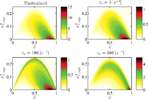
The precomputed filtered values of obtained using the UF model are stored in a look-up table with and σ²_{c, sgs} as controlling parameters. The SGS dissipation rate, , is used as a third parameter for the SF model. Typical variations of normalised by δ_th/s_L are shown in Figure 1 for the UF and SF models as a function of the controlling parameters. This result is shown for a stoichiometric methane–air flame since the validation case to be described in the next section uses this reactant mixture. The results are shown for three values of for the SF model. The maximum value of occurs around for very small values of σ²_{c, sgs}. For values around this , as the variance increases the filtered reaction rate decreases, which is because the burning part of the sub-grid PDF of c decreases as σ²_{c, sgs} increases, which is easy to verify using the Beta function employed for this study. For , the sub-grid PDF broadens as σ²_{c, sgs} increases which implies that the burning parts of the flamelet are seen occasionally leading to a relatively larger reaction rate as in Figure 1. The straining decreases the peak reaction rate substantially as one would expect. Except for this change, the variation of filtered reaction rate is similar for the unstrained and strained flamelets. These filtered values are used while computing the piloted Bunsen flames described next.

Figure 1. Typical variation of normalised filtered reaction rate in unstrained and strained flamelets.

3. Validation case

The piloted stoichiometric methane–air Bunsen flames of Chen et al. [33] were considered in several past RANS [24,30–32,62–66] and LES [7,26,28,39,40] studies using various combustion modelling approaches. The reactant jet has diameter D = 12 mm and issues into quiescent air as shown schematically in Figure 2. This jet is surrounded by a laminar, water-cooled pilot burner having a diameter of D_p = 68 mm and the burnt mixture is sub-adiabatic because of the heat loss to the burner. There is no turbulence generating device in the reactant flow path and thus the turbulence is shear driven. The three flames F1, F2, and F3 in [33], respectively, have a bulk mean velocity of U_b = 65, 50, and 35 m/s and the jet exit Reynolds number based on U_b and D is 52,000, 40,000 and 24,000, which were achieved in the experiments by varying only U_b. These flames belong to the thin reaction zones regime of premixed combustion [67] based on the centreline values of u′ and an integral length scale of Λ = 2.4 mm near the nozzle exit reported in [33].

Figure 2. A schematic of the experimental [33] and computational setups of the validation case.

The radial variation of averaged temperature, streamwise velocity, turbulent kinetic energy, and various species mass fractions at axial locations ranging from x/D = 2.5 to 10.5 were measured and reported in [33], which are useful to address the objectives of this study. Furthermore, these flames were considered in many past numerical studies using RANS and LES methodologies as noted earlier and thus a comparative evaluation can be made.

4. Large eddy simulation

The Favre filtered transport equations for conservation of mass and momentum are solved along with additional filtered equations required for combustion modelling. The additional quantities to be solved include the Favre filtered progress variable in Equation (4(4) ), the sub-grid variance in Equation (5(5) ), and the Favre filtered total enthalpy, , which is the sum of the sensible and chemical enthalpies of the mixture. The transport equation for , for mixtures with unity Lewis number, is (10)

The sub-grid stresses are modelled using the dynamic Smagorinsky model [68,69] and the SGS scalar fluxes are computed using the gradient hypothesis with the dynamic Schmidt number approach [69]. The test-filter size for all dynamic procedures used in this study is , following common practice, with the filter width estimated as Δ = (V_i)^1/3, where V_i is the volume of computational cell i.

Including the equation allows one to handle sub-adiabatic mixtures coming from the pilot stream of the test flames discussed in the previous section. The filtered temperature, , is obtained from the computed using , where is the specific heat capacity at constant pressure for the mixture and it depends on temperature as described in [52]. The mixture density is computed using the state equation: , where is the filtered pressure, is the Favre-filtered molecular weight of the mixture and is the universal gas constant. The values of , , and are specified as described below. First, the values of , , and are obtained using an equation similar to either Equation (1(1) ) or (9(9) ) with the respective flamelets. Then, the mixture values , , and are computed using a simple mixing rule given by (11) where and refer to one of the three quantities above and φ_air to their values in air, to include the mixing or dilution of burnt mixture with the entrained air. This mixing is less likely to cause partially premixed combustion at SGS level because the stoichiometric mixture issuing from the jet has sufficient oxygen to oxidise the CH₄ in the mixture and thus the experimental flames are expected to be purely premixed [39]. This dilution effect, however, will change the mass fractions, thermo-physical and thermo-chemical properties, and temperature of the burnt mixture as noted in [32]. Hence, the above mixing rule is used by tracking the fluid originating from the reactant and air streams using a filtered transport equation, similar to Equation (10(10) ), for a passive fluid marker, .

The required flamelet quantities are computed using the PREMIX [70] and Oppdiff [71] codes for unstrained and strained flamelets, respectively. The PREMIX code solves conservation equations for mass, momentum, energy, and species mass fractions for a freely propagating planar 1D laminar flame. Thus, there is no imposed strain acting on the flame. The Oppdiff code solves these conservation equations along the centreline of an opposed-jet flow configuration. The full form of these equations is given in [70–73]. The laminar flame stabilised near the stagnation plane is subjected to the fluid dynamic strain produced by the opposed jets and the influences of this strain on the flamelet is parameterised using the scalar dissipation rate in this study. Reactant-to-reactant and reactant-to-product jets are possible and the latter configuration is used for this study. Its relevance to turbulent premixed combustion has been discussed in many past studies, which are summarised in [32,60]. The combustion chemistry is represented using the GRI 3.0 mechanism in these flamelet calculations.

The fuel mass fraction, Y_f, is used here to define the instantaneous progress variable c = 1 − Y_f/Y_{f, u} so that it takes a value of 0 and 1 in reactants and products, respectively. The fuel mass fraction in the reactant is Y_{f, u}. This definition of c avoids spurious flames that would appear numerically in the mixing layer between the pilot and coflow if it were defined using temperature T or any other species mass fraction.

4.1. Numerical method and grid

The above conservation equations and the SGS closures are solved using PRECISE-MB code, which is based on finite volume methodology [74]. The spatial derivatives are discretised using a second order central differencing scheme and these equations are time advanced using a second order accurate scheme with a constant time step chosen to keep the CFL number smaller than 0.3 in the computational domain. Velocity–pressure coupling is achieved using the SIMPLEC algorithm [75].

A three-dimensional computational domain spanning 40D in the axial and radial directions as shown in Figure 2 is considered and is discretised using a structured multi-block grid having non-uniform numerical cells. These cells are finer near the burner exit and they grow gradually in the downstream and radial directions. A coarser grid having 22 cells inside the jet diameter, D, and about 4 cells within the turbulence integral length scale of Λ = 2.4 mm gives a total of about 1.5 million cells for the computational volume of π(40D)³/4. This grid has 404 cells in the streamwise direction and increasing the cell count to 32 for D and 6 for Λ, keeping other grid parameters almost the same, yielded about 4.2 million cells in total. These two grids, which are the same in [17], are used to assess the grid sensitivity of the LES results. The coarse grid having 1.5M cells satisfies the 80% turbulent energy criterion [55] and has Δ⁺_min ≈ 1.3, and the 4.2M grid has Δ⁺_min ≈ 0.8.

4.2. Boundary and initial conditions

The exit velocity for the jet is specified using its measured radial profile [33]. There is no fluctuation specified for this velocity since the turbulence in the reacting region is shear generated as noted in Section 3. However, one can use the digital filter [76] or the synthetic-eddy [77,78] method to prescribe turbulence for the inlet, if required. Analyses of cold flows discussed in the next section show that correct turbulence is recovered after few diameters downstream for the grid and other simulation parameters used in this study. A uniform velocity of 1.5 m/s is specified for the pilot stream on the basis of total volumetric flow rate obtained from the experimental data. A small velocity of 0.2 m/s is assigned to the coflowing air to mimic the air entrainment. The computed statistics are observed to be insensitive when this entrainment air velocity is changed by 25%.

The pilot stream temperature is unspecified in the experimental study and values ranging from 1785 to 2248 K were used in past studies [7,24,26,28,30–32,39,40,62–66] suggesting that the heat loss to the pilot burner varies from 0 [7] to 34% [28,64]. A value of 17% was used in [63] and 20% heat loss was assumed in [39,40]. For this study, it is taken to be 16% following [17,24,32], which gives 1950 K for the pilot temperature. These past studies showed that the pilot temperature uncertainty influences the temperature field only close to the jet exit (x ≤ 3D), which is also confirmed here by changing this temperature over a range of about 200 K.

The filtered progress variable, , has a value of zero in the jet exit and one for the pilot and coflowing streams. The σ²_{c, sgs} is specified to be zero in all of these boundaries as it is generated predominantly by chemical reactions inside the domain. The passive fluid marker, , is specified to be one at the jet and pilot exits, and zero for the air inlet. The total enthalpy at these boundaries is specified to be consistent with the respective temperature and mixture composition. The lateral boundaries are specified to be slip walls with zero normal scalar gradients and the outlet is set to have zero gradient in the streamwise direction for all the variables.

Large eddy simulations were conducted using 96 cores running on 2.60 GHz Intel Sandy Bridge E5-2670 processors on Darwin cluster at Cambridge University for about 18 flow-through times, which is defined using the computational domain length and the respective U_b. These computations took about 12 h on the wall clock for the 1.5M grid and 24 h for the 4.2M grid on the above cluster for about 18 flow-through times. These run times are about 30% longer compared with those reported in [17] for an algebraic closure of the filtered reaction rate. Statistics were collected for a period of about 16 flow-through times for each simulation, after the initial transients had left the domain, and this was substantially larger than what had been used in past studies of these flames. All the three flames, F1, F2, and F3, in [33] were simulated, but typical results are shown and discussed below using the F1 and F3 flames.

5. Results and discussion

5.1. Non-reacting flow

The LES results were time averaged first over the sampling period and then averaged in the azimuthal direction in order to get the radial variation of mean quantities at various axial positions as reported in the experimental study [33]. This averaging procedure, which is also density weighted when required [1], is denoted by using ⟨⋅⋅⋅⟩ in the following discussion.

The radial variations of axial mean velocity and turbulent kinetic energy are compared with measured values at five axial locations in Figure 3 for both the 1.5M and 4.2M grids. These quantities are normalised using U_b = 50 m/s and k₀ = 10.8 m²/s² for the flame F2. The turbulent kinetic energy (TKE), k, is obtained as k = 0.5∑⟨u_iu_i⟩ + 1.5⟨u′²_Δ⟩, where . These results suggest that the computational model represents experiments well and the difference between the 1.5M and 4.2M grid results are negligible as reported in [17]. However, some difference in ⟨k⟩ is observed for r ≤ 0.6D and this difference decreases as one moves in the downstream direction. As seen in Figure 3, the turbulence levels represented by ⟨k⟩ in regions r > 0.6D of combustion are captured quite well with no inlet turbulence, and specifying some inlet turbulence improves this comparison for x/D = 2.5 but no significant changes are observed for other downstream locations because the turbulence results predominantly from the shear generation mechanism in the jet flow configuration. These results demonstrate that the 1.5M grid is adequate to capture the flow dynamics and hence this grid is used for reacting flow calculations discussed next. Nevertheless, the 4.2M grid is also used for further testing if required.

Figure 3. Comparison of measured [33] (symbols) and computed, using 1.5M (solid line) and 4.2M (dotted line) grids, normalised mean axial velocity and turbulent kinetic energy in the cold flow of flame F2.

5.2. Reacting flows

The results obtained using unstrained and strained flamelets are compared and discussed in this section. The species mass fractions of major and minor species are discussed. Before comparing these two flamelet models, the sensitivity of the computational results to the numerical grid is discussed.

5.2.1. Grid sensitivity

The radial variation of various quantities such as ⟨U⟩, ⟨k⟩, fuel mass fraction, and normalised mean temperature is shown in Figures 4, 5, 6, and 7. The averaged velocity, turbulent kinetic energy, fuel mass fraction, and normalised temperature from flames F1 and F3 are shown for various streamwise positions. Although all three flames are computed, typical results are shown here for only the F1 and F3 flames because they have the extreme values of Da, Ka, and Re_t in the range investigated experimentally in [33]. The mean velocity is normalised using the respective U_b and the mean TKE is normalised using the values k₀ = 12.7 m²/s² for the F1 flame and 3.82 for the F3 flame reported in [33]. The normalised temperature is , where is the filtered temperature calculated using obtained from as described in Section 4 and the fuel mass fraction is constructed from the computed . The relationship between and is discussed in Section 5.2.2 A. Figures 6 and 7, to be discussed in detail later, compare computational results with the measurements (open circles) and representative results from previous studies employing other SGS combustion closures. For the discussion in this section, the focus is on the present computational results obtained using the 1.5M and 4.2M grids in reference to the experimental values; other results shown in these figures will be discussed in later sections.

Figure 4. Comparison of measured [33] (symbols) and computed (lines) radial variation of ⟨U⟩/U_b for the F1 and F3 flames. The unstrained flamelet result is shown for the 1.5M (

) and 4.2M (

) grids, and the strained flamelets result is shown for the 1.5M (

) and 4.2M (

) grids. The results for the 4.2M grid are shown only for the F1 flame.

Figure 5. Comparison of measured [33] (symbols) and computed (lines) radial variation of ⟨k⟩/k₀ for the F1 and F3 flames. See Figure 4 for legend.

Figure 6. The normalised mean temperature computed on the 1.5M grid using the UF (

) and SF (

) models is compared with measurements [33] (

). Previous results [7] (▵), [28] (), [32] (

) and [39] (

) are shown for comparison.

Figure 7. Comparison of measured [33] (

) and computed mean fuel mass fraction. The computational results are shown for the 1.5M grid using the UF (

) and SF (

) models. Previous results [7] (▵), [28] (), [32] (

) and [39] (

) are shown for comparison.

The mean velocity variations show that the 1.5M grid is adequate to capture the experimental results. The results for the 4.2M grid, shown only for F1, demonstrate that the mean velocity is not strongly sensitive to the numerical grids used here and in [17]. Similar behaviour is also observed for the SF model. The TKE results in Figure 5 also suggest a similar conclusion. However, the computed TKE results are relatively large for the SF model and show some sensitivity to the grid, as shown in Figure 5. Despite this, the general variation of TKE does not seem to be influenced by the numerical grid. The reason for the sensitivity observed for the strained flamelets model will become clearer when the results of unstrained and strained flamelets are discussed in the next subsection. The sensitivity (not shown) of mean mass fraction of methane and normalised temperature to the numerical grid is similar to that shown for ⟨U⟩. These results suggest that they are weakly sensitive to the numerical grids employed and second order quantities such as TKE show a sensitivity for the SF model. The results for the 1.5M grid are used for the subsequent analysis below because of the weak grid sensitivity observed for the mean quantities.

5.2.2. Unstrained versus strained flamelets

The results in Figure 4 show that the heat release induced acceleration in the flame F3 having the highest Da is underestimated by the SF model compared with the UF model for the upstream positions, x/D = 2.5 and 4.5. This implies that the local burning rate is underestimated by the SF model, which will be further confirmed later through Figures 8 and 9. However, this difference becomes negligible as one moves downstream. Similar observations are made for F1 having the highest Re_t and lowest Da.

Figure 8. Spatial variation of in flame F3 obtained at an arbitrarily chosen time, t1, using (a) the UF and (b) the SF model with the 1.5M grid. These results at 20 ms later are shown in (c) and (d). The contours are shown for .

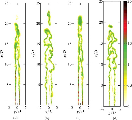
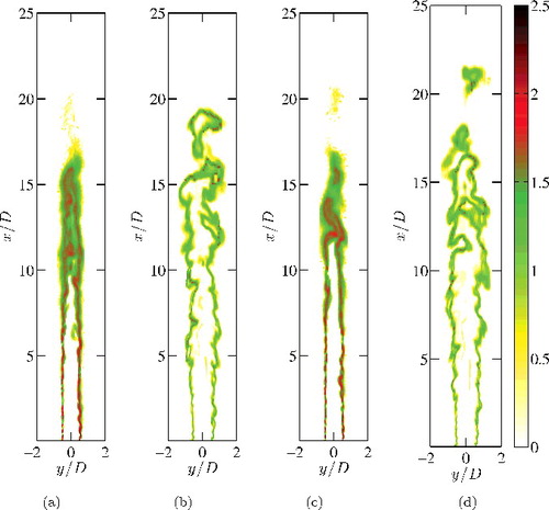
Figure 9. Spatial variation of in flame F1 obtained at an arbitrarily chosen time, t1, using (a) the UF and (b) the SF model with the 1.5M grid. These results at 20 ms later are shown in (c) and (d). The contours are shown for .

The normalised mean TKE obtained using these two models is compared in Figure 5 with the experimental data. The trends obtained using them are similar for the flame F3 and there is some over estimation of ⟨k⟩ in the flame region, 0.55 ≤ r/D ≤ 0.7. The values obtained using the SF model are generally larger and the UF results compare favourably with the measurements for the F1 flame as seen in Figure 5. A closer study of this figure suggests that the shear layer, where the filtered flame is expected to reside, is shifted slightly towards the centreline, which is suggested by the shift in the peak value of ⟨k⟩. The production of TKE by the fluid dynamic shear is likely to be aided by the radial acceleration of the fluid resulting from heat release effects. Because of these effects, ⟨k⟩ is overestimated for r/D ≤ 0.6 as observed in Figure 5. Nevertheless, the comparisons shown here for the UF model are very similar to those observed in earlier studies using various SGS [7,26,28,39,40] and RANS [17,24,30–32,62–66] combustion modelling approaches.

The spatial variation of filtered reaction rate for the UF and SF models are compared in Figures 8 and 9 for F3 and F1, respectively. These results are shown for two different times as for , where is the normalised filtered reaction rate. The maximum observed is about 2.63 and the logarithm is used here to depict the spatial variations clearly because the combustion is a small-scale phenomenon. Laminar-like structure with negligible wrinkling is observed in F3 having the highest Da for the UF model. If the strain effects are included then the influence of shear layer roll-up resulting from the Kelvin–Helmholtz instability on the filtered flame becomes apparent, as shown in Figure 8 for the two arbitrary time instances. Also, the peak reaction rate occurs near the jet exit and this value is reduced considerably (see Figure 1) as one would expect when stretching effects are included. The overall flame length is more or less the same and there is island formation as in Figure 8 for the two combustion models used.

Although the peak reaction rate is reduced for the SF model, the overall mean burning rate is maintained by the increase in flame area resulting from the increased level of flame wrinkling compared with the UF model. The overall mean burning rate and thus the mean heat release rate given by , where ΔH_c is the heat of combustion, must be the same for both models because the fuel flow rate, , is identical and there are no local extinctions. Despite this, a distinct difference is observed for F1 having the highest Re_t and lowest Da as seen in Figure 9. The peak reaction rate is spatially intermittent in Figure 9(a) and an indication of temporal intermittency is seen by comparing Figures 9(a) and 9(c). These intermittencies are expected in high Re_t flames. The most apparent difference between the filtered reaction rates computed using the UF and SF models is seen for F1 in the region of x/D ≥ 10. The SF model confines the reaction rate to thin layers all the way to x/D ≈ 15, whereas the reaction rate is distributed more or less uniformly over a larger region for x/D ≥ 11 when the UF model is used. A small change in the size of this region is observed if one compares Figure 9(a) with 9(c). It is not easy to comment which one of the behaviours in Figures 8 and 9 for the UF and SF models is correct because the experimental study [33] did not report reaction rate. Furthermore, it is not too easy to measure reaction rate quantitatively, but it is possible to image surrogates of reaction rate qualitatively using laser diagnostics for the OH, CH₂O and CH species. In the absence of such information, one can compare and analyse statistics gathered from the experimental and past and current numerical studies for further assessment. The comparisons discussed above for the mean velocity suggest that both the UF and SF models are good but the TKE variation suggests that the UF model may be preferred. One must also investigate the behaviour of scalar mass fractions, which is conducted next.

A. Major species

The radial variations of mean fuel mass fraction and normalised temperature are compared with measurements and past numerical results in Figure 7. The results are shown for various streamwise positions in the F1 and F3 flames. The averaged fuel mass fraction computed using the UF model is lower than the measured values for 0.5 ≤ r/D ≤ 0.7 at x/D = 2.5 for both F1 and F3 shown in Figure 7. The estimates obtained using the SF model are relatively better for this location. However, the UF values are closer to the measurements compared with the SF results at downstream locations. Indeed, the SF model overestimates the averaged fuel mass fraction and the level of this overestimation increases with downstream distance for both the F1 and F3 flames. This is consistent with the reaction rate behaviour shown in Figures 8 and 9. The results in Figure 7 suggest that the UF model predictions are comparable with those obtained using other combustion modelling approaches such as the thickened flames [7,39] and Eulerian stochastic fields methods [28].

The normalised mean temperature variation with normalised radius is shown in Figure 6 for the flames F1 and F3 at various axial positions. The mean temperature is obtained by calculating using the expression proposed in [32]. The symbol σ²_T denotes the total variance, which is the sum of resolved and SGS variances. The SGS part is obtained as σ²_{T, sgs} ≃ σ²_{c, sgs}. No significant difference is observed between and , and thus the mean temperature is denoted using ⟨T⁺⟩ in the following discussion. The significant overestimate at x/D = 2.5 is because of the uncertainty in the boundary condition for the pilot stream and this overestimate was also observed in past studies as depicted in Figure 6. This overestimate decreases as one moves downstream for both the F1 and F3 flames. The relative behaviour of the UF and SF models is consistent with that for the fuel mass fraction. Although the SF model gives a good comparison for x/D = 6.5 for the F1 flame, it underestimates the peak temperature for downstream positions and the level of under-prediction increases gradually with downstream distance, as shown in Figure 6, whereas the UF model prediction improves with distance and is comparable with previous results and measurements. The difference between these two models is small for F3 having the highest Da.

Figure 10 compares the computed values of mean mass fraction of H₂O with the measurements [33] and results of previous studies. The results of both models are shown in this figure and the SF model under-predicts the mean mass fraction of water vapour, which is consistent with the fuel mass fraction variation discussed earlier. Results of the UF model are close to the measurements for all the axial positions in both F1 and F3 flames. Also, one observes in Figure 10 that the UF model predictions are improved compared with some of the earlier studies employing nearly three to four times the total grid size used in the current study. This is for the following reasons:

Figure 10. Comparison of measured [33] and computed mean mass fraction of H₂O. The legend is as shown in Figure 7.

(i)	the UF modelling framework used here does not have arbitrary or tuneable model parameters as noted in Section 2.1,
(ii)	the various SGS models, Equations (1(1) ), (6(6) ), and (7(7) ), related to combustion are consistent with one another,
(ii)	the SGS variance is obtained through its transport equation to maintain consistency among important physical processes for production and dissipation of progress variable fluctuations, and
(iv)	the dissipation rate model and its parameters are linked to the physical aspects of the problem so that the model response is consistent with the change in local processes.

Elaborate discussion on the SGS variance is given in Section 5.3. Comparisons for other major species such as O₂ and CO₂ are similar to those shown here for water vapour and fuel and thus they are not shown here.

B. Minor species

Figures 11 and 12, respectively, compare the radial variations of the mass fractions of the minor species OH and H₂ with the results of past studies and measurements. The results of past studies are shown in these figures only if they were reported. There is a severe under-prediction by the SF model, whereas the UF model yields good predictions of the minor species mass fractions for both the F1 and F3 flames. The OH mass fraction comparison shown in Figure 11 is much better than the comparison shown in [17, Figure 15] for an algebraic reaction rate closure based on high Da combustion. This improved comparison is because these flamelet models can handle finite rate chemistry effects for the filtered reaction rate. This is also reflected in the H₂ mass fraction comparison shown in Figure 12. The results presented so far suggest that the UF model performs consistently better compared with the SF model, which is interesting because [32] suggested that the SF model was required for correct prediction of these piloted Bunsen flames using RANS methodology.

Figure 11. Comparison of measured [33] and computed OH mass fractions. The legend is as shown in Figure 7.

Figure 12. Comparison of measured [33] and computed H₂ mean mass fractions. The legend is as shown in Figure 7.

The under-prediction seen here for the SF model is because of under-prediction of filtered burning rate observed in Figures 8 and 9. When the flame front is stretched by turbulent eddies through straining and bending (curvature), the burning rate drops. These effects are parameterised through the SGS dissipation rate, , in the SF model used here (see Section 2.2). The majority of energy containing eddies is tracked through resolved scales in typical LES, as is that reported here, and thus their flame stretching is included inherently through , σ²_{c, sgs}, and the enthalpy transport equations and their interactions. So, attempting to include flame stretching caused by SGS eddies that are too weak to influence the flame (see Section 1: ‘Introduction’) will over-compensate for the flame stretching effects. However, these effects may not be small if LES is under resolved but this is not the case for this study (see Section 4.1). Thus, using the SF model to capture SGS flame stretching overestimates these effects leading to substantial reduction in the burning rate. Hence, there may not be a need to include SGS flame stretching in a typical (or practical) LES as these eddies are expected to be too weak to stretch filtered flames.

It is also important to note that the SGS variance of the progress variable is computed here using its transport equation rather than through a commonly used model, to include correct and meaningful interactions among turbulence, scalar mixing, and reactive fields. The reasons for this are discussed next.

5.3. Role of SGS variance

The SGS progress variable equation written earlier as Equation (5(5) ) is rewritten below for convenience as (12) The terms T₁ and T₂ are the unsteady and advective terms, respectively. The molecular and turbulent fluxes of σ²_{c, sgs} are T₃₁ and T₃₂, respectively. The terms T₄, T₅, and T₆ signify the SGS chemical processes, dissipation of σ²_{c, sgs}, and its production through interaction of the SGS scalar flux and the gradient of , respectively. It is important to recognise these physical processes in order to evaluate the validity of the commonly used model for σ²_{c, sgs}, which is obtained by equating T₅ and T₆ after approximating the dissipation rate as . This model for is based on a linear relaxation hypothesis using the SGS turbulence timescale [46,79]. As will be seen below, these models for and σ²_{c, sgs} should not be used for LES of premixed flames as they exclude the influences of combustion.

The above transport equation is studied using an order of magnitude analysis as follows. The spatial derivatives of filtered quantities, time derivatives, and density are scaled using Δ, Δ/U_ref, and ρ_u, respectively. The filtered velocity is scaled using a reference velocity U_ref. The molecular diffusivity is scaled using the laminar flame scales, s_L and δ_th, and the SGS viscosity is scaled as u′_Δ Δ. The progress variable gradient is produced predominantly by the chemical reaction and thus the appropriate scaling for is s_L/δ_th. However, one can also scale this term using u′_Δ/Δ if the combustion effects are ignored and the SGS turbulence is presumed to be responsible for the progress variable gradient which can occur through mixing of unburnt and burnt mixtures. 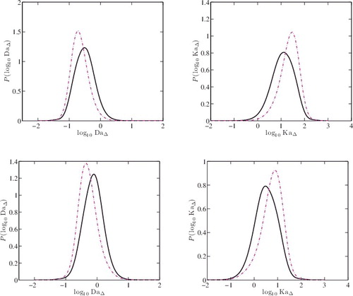The above scalings yield (13) (14) (15) where Re_Δ = u′_ΔΔ/(s_Lδ_th) is the SGS Reynolds number. If the local SGS Damköhler number is large, then the leading order balance is between T₄ and T₅ which implies that , suggesting that the SGS variance is proportional to Da_Δ. However, the PDFs of Da_Δ and Ka_Δ shown in Figure 13, which will be discussed in detail in Section 5.4, for both F1 and F3, suggest that this Damköhler number is finite and thus the other terms in the balance equation cannot be neglected. If one takes a balance among sources and sinks as is typically done in non-reacting flows, then T₅ ≃ T₄ + T₆, which would give , where is a model parameter. This balance is unacceptable because other terms in Equation (12(12) ) will be of similar magnitude since they have the same dependence on Da_Δ.

Figure 13. PDFs of Da_Δ and Ka_Δ from flames F1 (top row) and F3 (bottom row). The results are shown for the UF (

) and the SF (

) models.

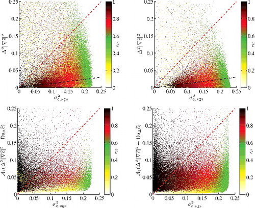
As noted earlier, the commonly used model is obtained through T₅ ≃ T₆, which can be justified only if (u′_Δ/Δ) is used to scale . This specific scaling gives

and ignores the important aspect of premixed combustion, i.e. the progress variable gradient is produced predominantly by combustion, which is also recognised in an earlier study investigating the SGS variance and dissipation rate of a conserved scalar [36]. This implies that the commonly used model will underestimate σ²_{c, sgs}, which is verified in Figure 14 for the F1 flame using both the 1.5M and 4.2M grids at an arbitrarily chosen time t1 (the same as in Figures 8 and 9) by plotting σ²_{c, sgs, model} with σ²_{c, sgs} and colouring the data points using the value. The results for F3 (also the SF model) are similar and thus they are not shown here. If the modelled value agrees with σ²_{c, sgs} then the data must cluster around the diagonal line (). The data seems to cluster predominantly around the dash–dotted line, which has a slope of about 0.125 suggesting that . The more apparent clustering for the 4.2M grid is because of reduced scatter. It is clear that the model σ²_{c, sgs, model} underestimates the variance as suggested by the above scaling analysis.

Figure 14. Scatter plot of computed σ²_{c, sgs} and its modelled value using with in the top row. The results for the revised model, with , are shown in the bottom row. The first and second columns are for the 1.5M and 4.2M grids of the F1 flame, respectively.

Values of σ²_{c, sgs, model} smaller than σ²_{c, sgs} will give larger for for the UF model (see Figure 1). This overestimate of coming from the (incorrectly modelled) SGS variance implies that flame stretching from SGS eddies needs to be considered. If one uses the SF model to include this stretching and σ²_{c, sgs}, then the filtered burning rate is severely underestimated leading to substantial underestimate of various reactive scalar mass fractions as observed in earlier sections of this paper. If one uses the incorrect variance, σ²_{c, sgs, model}, then the SF model results may improve. This is not attempted here because σ²_{c, sgs, model} does not contain the essential physical aspects of premixed combustion and thus it would be misleading.

If one were to use the revised algebraic model, σ²_{c, sgs, model1}, then the SGS variance would be severely overestimated because Da_Δ varies from to yielding σ²_{c, sgs, model1} substantially larger than its maximum limit of 0.25. Indeed this overestimate can be seen in the bottom row of Figure 14 for both the grids if one were to use instead of 0.15 as used for this figure. This substantial overestimate suggests that the transport terms in Equation (12(12) ) should not be neglected to get meaningful values for the SGS variance and this equation needs to be included for the LES of premixed combustion using the UF model. The additional computational cost incurred by including this transport equation is small, which is fully justified through correct representation of turbulent premixed combustion physics as discussed above.

To summarise, the SGS variance and its modelling consistent with the physical aspects of premixed combustion play a central role in the presumed PDF-based flamelet closure for the filtered reaction rate. If the SGS variance, σ²_{c, sgs}, is computed using its transport equation with consistent SGS closures in a practical LES, then the UF model would be adequate and the SF model may not be required. This can only be assessed further by applying the UF model and its framework discussed here for premixed combustion in various configurations and regimes. These tests will be reported in future studies.

5.4. Discussion

Figure 13 suggests that the typical values of range from about 0.1 to 1.8 in F1 and 0.16 to 5 in F3 flames. These ranges are not strongly influenced by flame stretching effects included in the SF model, except that the most probable value is reduced slightly. The relative behaviour between the UF and SF models does not seem to vary between the F1 and F3 flames, which is consistent with the flame statistics discussed earlier. The variation of the PDF is similar and consistent with the PDF of . These two PDFs are more or less symmetric about the most probable value, suggesting that they may be lognormal. However, the PDF shows a slightly longer negative tail because of the nonlinear dependence on the small-scale quantities.

The scale-dependent β_c in Equation (7(7) ) is an important parameter in the SGS combustion modelling approach used in this study. This parameter is obtained dynamically using scale-similarity [17] as noted in Section 2.1 and it varies spatio-temporally. The PDF of β_c is shown in Figure 15 for both the F1 and F3 flames. These PDFs are constructed using β_c values collected from the entire computational domain and 50 snapshots in time, and by imposing the limits and to avoid regions with very low reaction rates so that the values of β_c used for this PDF are physically meaningful. This was verified in [17] in conjunction with an algebraic reaction rate closure. The PDFs shown here for the UF and SF models are similar to those in Langella et al. [17, Figure 18], except for a lower limit used in that study. The lower limit was set to satisfy a realisability condition of , which was obtained by analysing the transport equation for the mean scalar dissipation rate [54]. For the reaction rate closures used in this study, the realisability condition for the filtered dissipation rate, , is met if C₃ ≥ τ C₄Da_Δ, see Equation (7(7) ), which is satisfied automatically by the functional forms of C₃ and C₄ described in Section 2.1.

Figure 15. The PDF of β_c from (a) flame F1 and (b) flame F3 obtained using the UF (

) and SF (

) models with the 1.5M grid.

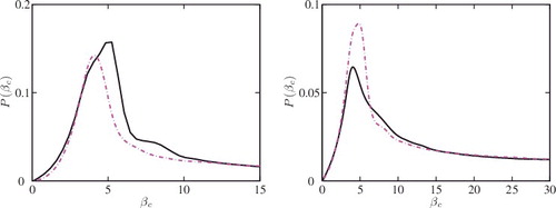
The PDF of β_c is shown for both UF and SF models for the 1.5M grid simulations. These results for the 4.2M grid are very similar to those shown here. There are no differences between these two models, and thus the flame stretching effects from SGS eddies introduced through strained flamelets do not influence the physical processes described by the β_c parameter.

6. Summary and conclusion

Large eddy simulation of premixed combustion is conducted using unstrained and strained flamelets for sub-grid scale combustion. The required sub-grid PDF of the progress variable is presumed using the Beta function, and the SGS variance, σ²_{c, sgs}, is obtained from its modelled transport equation. The contribution of combustion in this equation is closed in a manner consistent with the closure for the filtered reaction rate. The SGS scalar dissipation rate is modelled using an algebraic model proposed in [18] and investigated in [17,19]. Two grids of 1.5M and 4.2M are employed and these grids resolve more than 80% of turbulent kinetic energy and show a negligible difference in the computed mean velocity and turbulent kinetic energy, and also compare well with the measured values for cold flows of the piloted Bunsen flames in [33].

The averaged streamwise velocity and various scalar mass fractions including temperature obtained using the UF and SF models show a weak sensitivity to the numerical grid, but the TKE computed using the SF model shows a substantial sensitivity, which is observed to be weak for the UF model. There is substantial difference between the results obtained using these two closures. The stretching of SGS turbulence is parameterised using the SGS dissipation rate in the SF closure. Since the numerical grids employed for the simulations resolve most of the turbulent kinetic energy, the SGS kinetic energy is expected to be small – implying that the SGS eddies are too weak to stretch the flame, which is similar to the views expressed by Poinsot et al. [37] and Roberts et al. [38] while investigating turbulent combustion regimes. Thus, using the SGS dissipation rate or any other parameter to parameterise the SGS flame stretching will overcompensate these effects compared with the influences of resolved eddies on the unstrained flamelet. Hence, the burning rate is underestimated by the SF model leading to the overestimation of fuel mass fraction and the underestimation of various reactive scalar mass fractions. The influences of resolved dynamic scales are included inherently in the UF closure through various transport equations and their interactions.

The SGS variance equation plays an important role in this aspect, and using an algebraic closure for σ²_{c, sgs} is incorrect, which is demonstrated using order of magnitude analysis of the SGS variance equation. The commonly used model severely underestimates the SGS variance because it excludes the leading order combustion effects. This underestimated variance will give a larger reaction rate for the UF closure (see Figure 1) implying a need for strained flamelets. Also, a model based on a linear relaxation hypothesis for excludes combustion effects and thus it is inappropriate for premixed combustion as noted in Section 5.3. The results presented in this paper suggest that the UF model works well, at least for the conditions investigated here, if one pays close attention to the modelling of σ²_{c, sgs} to retain the important subtleties of premixed combustion physics consistently across various SGS closures. Applying this modelling framework to other flame configurations and combustion regimes would be useful to assess the findings of this study further, and this will be explored in subsequent investigations.

Disclosure statement

No potential conflict of interest was reported by the authors.

Additional information

Funding

The authors express their gratitude to EPSRC [grant number EP/I027556/1], Siemens and Rolls-Royce for their support. The numerical data used in this study may be obtained by contacting the corresponding author.

References

- T.J. Poinsot and D. Veynante, Theoretical and Numerical Combustion, R.T. Edwards, Philadelphia, PA, 2005.
- H. Pitsch, Large-eddy simulation of turbulent combustion, Annu. Rev. Fluid Mech. 38 (2006), pp. 453–482.
- L.Y.M. Gicquel, G. Staffelbach, and T. Poinsot, Large eddy simulations of gaseous flames in gas turbine combustion chambers, Prog. Energy Combust. Sci. 38 (2012), pp. 782–817.
- N. Swaminathan and K.N.C. Bray, Fundamentals and challenges, in Turbulent Premixed Flames, N. Swaminathan and K.N.C. Bray, eds., Cambridge University Press, Cambridge, UK, 2011, pp. 1–40.
- R.S. Cant, RANS and LES modelling of turbulent combustion, in Turbulent Combustion Modelling: Advances, New Trends and Perspectives, T. Echekki and E. Mastorakos, eds., Springer, Heidelberg, 2011, pp. 63–87.
- O. Colin, F. Ducros, D. Veynante, and T.J. Poinsot, A thickened flame model for large eddy simulations of turbulent premixed combustion, Phys. Fluids 12 (2000), pp. 1843–1863.
- A. De and S. Acharya, Large eddy simulation of a premixed Bunsen flame using a modified thickened-flame model at two Reynolds numbers, Combust. Sci. Technol. 181 (2009), pp. 1231–1272.
- M. Boger, D. Veynante, H. Boughanem, and A. Trouvé, Direct numerical simulation analysis of flame surface density concept for large eddy simulation of turbulent premixed combustion, Proc. Combust. Inst. 27 (1998), pp. 917–925.
- E.R. Hawkes and R.S. Cant, Implications of a flame surface density approach to large eddy simulation of premixed turbulent combustion, Combust. Flame 126 (2001), pp. 1617–1629.
- R. Knikker, D. Veynante, and C. Meneveau, A dynamic flame surface density model for large eddy simulations of turbulent premixed combustion, Phys. Fluids 16 (2004), Paper No. L91. http://dx.doi.org/10.1063/1.1780549.
- N. Chakraborty and R.S. Cant, A priori analysis of the curvature and propagation terms of the flame surface density transport equation for large eddy simulation, Phys. Fluids 19 (2007), Paper No. 105101. http://dx.doi.org/10.1063/1.2772326.
- N. Chakraborty and M. Klein, A priori direct numerical simulation assessment of algebraic flame surface density models for turbulent premixed flames in the context of large eddy simulation, Phys. Fluids 20 (2008), Paper No. 085108. http://dx.doi.org/10.1063/1.2969474.
- S.R. Gubba, S.S. Ibrahim, and W. Malalasekera, Dynamic flame surface density modelling of flame deflagration in vented explosion, Combust. Expl. Shock Waves 48 (2012), pp. 393–405.
- G. Wang, M. Boileau, D. Veynante, and K. Truffin, Large eddy simulation of a growing turbulent premixed flame kernel using a dynamic flame surface density model, Combust. Flame 159 (2012), pp. 2742–2754.
- H. Pitsch, A consistent level set formulation for large-eddy simulation of premixed turbulent combustion, Combust. Flame 143 (2005), pp. 587–598.
- V. Moureau, B. Fiorina, and H. Pitsch, A level set formulation for premixed combustion LES considering the turbulent flame structure, Combust. Flame 156 (2008), pp. 801–812.
- I. Langella, N. Swaminathan, Y. Gao, and N. Chakraborty, Assessment of dynamic closure for premixed combustion LES, Combust. Theory Model. 19 (2015), pp. 628–656.
- T.D. Dunstan, Y. Minamoto, N. Chakraborty, and N. Swaminathan, Scalar dissipation rate modelling for large eddy simulation of turbulent premixed flames, Proc. Combust. Inst. 34 (2013), pp. 1193–1201.
- Y. Gao, N. Chakraborty, and N. Swaminathan, Algebraic closure of scalar dissipation rate for large eddy simulations of turbulent premixed combustion, Combust. Sci. Technol. 186 (2014), pp. 1309–1337.
- T. Ma, Y. Gao, A.M. Kempf, and N. Chakraborty, Validation and implementation of algebraic LES modelling of scalar dissipation rate for reaction rate closure in turbulent premixed combustion, Combust. Flame 161 (2014), pp. 3134–3153.
- D. Butz, Y. Gao, A.M. Kempf, and N. Chakraborty, Large eddy simulations of a turbulent premixed swirl flame using an algebraic scalar dissipation rate closure, Combust. Flame 162 (2015), pp. 3180–3196.
- A.Y. Klimenko and R.W. Bilger, Conditional moment closure for turbulent combustion, Prog. Energy Combust. Sci. 25 (1999), pp. 595–687.
- S.M. Martin, J.C. Kramlich, G. Kosaly, and J.J. Riley, The premixed conditional moment closure method applied to idealized lean premixed gas turbine combustors, J. Eng. Gas Turbines Power 125 (2003), pp. 895–900.
- S. Amzin, N. Swaminathan, J.W. Rogerson, and J.H. Kent, Conditional moment closure for turbulent premixed flames, Combust. Sci. Technol. 184 (2012), pp. 1743–1767.
- S. Amzin and N. Swaminathan, Computations of turbulent lean premixed combustion using CMC, Combust. Theory Model. 17 (2013), pp. 1125–1153.
- S.L. Yilmaz, M.B. Nik, P. Givi, and P.A. Strakey, Scalar filtered density function for large eddy simulation of a Bunsen burner, J. Propulsion & Power 26 (2010), pp. 84–93.
- D.H. Rowinski and S.B. Pope, Computational study of lean premixed turbulent flames using RANSPDF and LESPDF methods, Combust. Theory Model. 17 (2013), pp. 610–656.
- I.A. Dodoulas and S. Navarro-Martinez, Large eddy simulation of premixed turbulent flames using the probability density function approach, Flow Turbul. Combust. 90 (2013), pp. 645–678.
- G. Bulat, W.P. Jones, and A.J. Marquis, NO and CO formation in an industrial gas-turbine combustion chamber using LES with the Eulerian sub-grid PDF method, Combust. Flame 161 (2014), pp. 1804–1825.
- M. Salehi and W. Bushe, Presumed PDF modelling for RANS simulation of turbulent premixed flames, Combust. Theory Model. 14 (2010), pp. 381–403.
- M. Salehi, W. Bushe, and K. Daun, Application of the conditional source term estimation for turbulence chemistry interactions in a premixed flame, Combust. Theory Model. 16 (2012), pp. 301–320.
- H. Kolla and N. Swaminathan, Strained flamelets for turbulent premixed flames II: Laboratory flame results, Combust. Flame 157 (2010), pp. 1274–1289.
- Y.C. Chen, N. Peters, G.A. Schneemann, N. Wruck, U. Renz, and M.S. Mansour, The detailed structure of highly stretched turbulent premixed methane–air flames, Combust. Flame 107 (1996), pp. 223–244.
- C. Meneveau and T. Poinsot, Stretching and quenching of flamelets in premixed turbulent combustion, Combust. Flame 86 (1991), pp. 311–332.
- E. Knudsen, H. Kolla, E.R. Hawkes, and H. Pitsch, LES of a premixed jet flame DNS using a strained flamelet model, Combust. Flame 160 (2013), pp. 2911–2927.
- C.D. Pierce and P. Moin, A dynamic model for subgrid-scale variance and dissipation rate of a conserved scalar, Phys. Fluids 10 (1998), pp. 3041–3044.
- T. Poinsot, D. Veynante, and S. Candel, Quenching processes and premixed turbulent combustion diagrams, J. Fluid Mech. 228 (1991), pp. 561–606.
- W.L. Roberts, J.F. Driscoll, M.C. Drake, and L.P. Goss, Images of the quenching of a flame by a vortex – To quantify regimes of turbulent combustion, Combust. Flame 94 (1993), pp. 58–62. http://dx.doi.org/10.1016/0010-2180(93)90019-Y.
- G. Wang, M. Boileau, and D. Veynante, Implementation of a dynamic thickened flame model for large eddy simulations of turbulent premixed combustion, Combust. Flame 158 (2011), pp. 2199–2213.
- H. Pitsch and L. de Lagneste, Large-eddy simulation of a premixed turbulent combustion using level-set approach, Proc. Combust. Inst. 29 (2002), pp. 2001–2208.
- A.W. Cook and J.J. Riley, A subgrid model for equilibrium chemistry in turbulent flows, Phys. Fluids 6 (1994), pp. 2868–2870.
- B. Fiorina, R. Vicquelin, P. Auzillon, N. Darabiha, O. Gicquel, and D. Veynante, A filtered tabulated chemistry model for LES of premixed combustion, Combust. Flame 157 (2010), pp. 465–475. http://dx.doi.org/10.1016/j.combustflame.2009.09.015.
- P. Domingo, L. Vervisch, S. Payet, and R. Hauguel, DNS of a premixed turbulent V flame and LES of a ducted flame using a FSD-PDF subgrid scale closure with FPI-tabulated chemistry, Combust. Flame 143 (2005), pp. 566–586.
- A.W. Vreman, J.A. van Oijen, L.P.H. de Goey, and R.J.M. Bastiaans, Subgrid scale modeling in large-eddy simulation of turbulent combustion using premixed flamelet chemistry, Flow Turbul. Combust. 82 (2009), pp. 511–535.
- V. Moureau, P. Domingo, and L. Vervisch, From large-eddy simulation to direct numerical simulation of a lean premixed swirl flame: Filtered laminar flame – PDF modeling, Combust. Flame 158 (2011), pp. 1340–1357.
- G. Lecocq, S. Richard, O. Colin, and L. Vervisch, Hybrid presumed PDF and flame surface density approaches for large-eddy simulation of premixed turbulent combustion Part 1: Formalism and simulation of a quasi-steady burner, Combust. Flame 158 (2011), pp. 1201–1214.
- H. Kolla, J.W. Rogerson, N. Chakraborty, and N. Swaminathan, Scalar dissipation rate modeling and its validation, Combust. Sci. Technol. 181 (2009), pp. 518–535.
- N. Chakraborty and N. Swaminathan, Influence of the Damköhler number on turbulence–scalar interaction in premixed flames. II. Model development, Phys. Fluids 19 (2007), Paper No. 045104. http://dx.doi.org/10.1063/1.2714076.
- Y. Gao, N. Chakraborty, and N. Swaminathan, Scalar dissipation rate transport in the context of LES for turbulent premixed flames with non-unity Lewis number, Flow Turbul. Combust. 93 (2014), pp. 461–486.
- N. Swaminathan, G. Xu, A.P. Dowling, and R. Balachandran, Heat release rate correlation and combustion noise in premixed flames, J. Fluid Mech. 681 (2012), pp. 80–115.
- I. Ahmed and N. Swaminathan, Simulation of spherically expanding turbulent premixed flames, Combust. Sci. Technol. 185 (2013), pp. 1509–1540.
- S. Ruan, N. Swaminathan, and O. Darbyshire, Modelling of turbulent lifted jet flames using flamelets: A priori assessment and a posteriori validation, Combust. Theory Model. 18 (2014), pp. 295–329.
- I. Ahmed and N. Swaminathan, Simulation of turbulent explosion of hydrogen–air mixtures, Int. J. Hydr. Energy 39 (2014), pp. 80–115.
- N. Chakraborty, J.W. Rogerson, and N. Swaminathan, A priori assessment of closures for scalar dissipation rate transport in turbulent premixed flames using direct numerical simulation, Phys. Fluids 20 (2008), Paper No. 045106. http://dx.doi.org/10.1063/1.2903846.
- S.B. Pope, Turbulent Flows, Cambridge University Press, Cambridge, UK, 2000.
- D.K. Lilly, The representation of small-scale turbulence in numerical simulation experiments, in Proceedings of the IBM Scientific Computing Symposium on Environmental Sciences, 14–16 November 1966, Yorktown Heights, New York, H.H. Goldstine, ed., IBM, 1967, pp. 195–210.
- J. Bardina, J.H. Ferziger, and W.C. Reynolds, Improved subgrid scale models for large-eddy simulation, in Proceedings of the 13th Fluid and Plasma Dynamics Conference, 14–16 July 1980, Snowmass, CO, AIAA Paper 80-1357.
- J.H. Ferziger, Large eddy simulation: An introduction and perspective, in New Tools in Turbulence Modelling, O. Métais and J.H. Ferziger, eds., Springer-Verlag, Berlin, 1997, pp. 29–47.
- Y. Gao, N. Chakraborty, and N. Swaminathan, Dynamic closure of scalar dissipation rate for large eddy simulations of turbulent premixed combustion: A direct numerical simulations analysis, Flow Turbul. Combust. 95 (2015), pp. 775–802. http://dx.doi.org/10.1007/s10494-015-9631-3.
- H. Kolla and N. Swaminathan, Strained flamelets for turbulent premixed flames. I: Formulation and planar flame results, Combust. Flame 157 (2010), pp. 943–954.
- P.A. Libby and F.A. Williams, Structure of laminar flamelets in premixed turbulent flames, Combust. Flame 44 (1982), pp. 287–303.
- R.O.S. Prasad and J.P. Gore, An evaluation of flame surface density models for turbulent premixed jet flames, Combust. Flame 116 (1999), pp. 1–14.
- M. Herrmann, Numerical simulation of turbulent Bunsen flames with a level set flamelet model, Combust. Flame 145 (2006), pp. 357–375.
- R.P. Lindstedt and E.M. Vaos, Transported PDF modeling of high-Reynolds-number premixed turbulent flames, Combust. Flame 145 (2006), pp. 495–511.
- M. Stöllinger and S. Heinz, PDF modelling and simulation of premixed turbulent combustion, Monte Carlo Meth. Appl. 14 (2008), pp. 343–377.
- M. Stöllinger and S. Heinz, Evaluation of scalar mixing and time scale models in PDF simulations of a turbulent premixed flame, Combust. Flame 157 (2010), pp. 1671–1685.
- N. Peters, Turbulent Combustion, Cambridge Monographs on Mechanics, Cambridge University Press, Cambridge, UK, 2000. http://dx.doi.org/10.1017/CBO9780511612701.
- M. Germano, U. Piomelli, P. Moin, and W.H. Cabot, A dynamic subgrid-scale eddy viscosity model, Phys. Fluids A: Fluid Dynam. 3 (1991), pp. 1760–1765. http://dx.doi. org/10.1063/1.857955.
- D. Lilly, A proposed modification of the Germano subgrid scale closure method, Phys. Fluids A: Fluid Dynam. 4 (1992), pp. 633–635. http://dx.doi.org/10.1063/1.858280.
- R.J. Kee, J.F. Grcar, M.D. Smooke, and J.A. Miller, A Fortran program for modeling steady laminar one-dimensional premixed flames, Tech. Rep. SAND85-8240, Sandia National Laboratories, Livermore, CA, 1985.
- A.E. Lutz, R.J. Kee, J.F. Grcar, and F.P. Rupley, Oppdif: A Fortran program for computing opposed-flow diffusion flames, Tech. Rep. SAND96-8243, Sandia National Laboratories, Livermore, CA, 1997.
- M.D. Smooke and V. Giovangigli, Formulation of the premixed and nonpremixed test problems, in Reduced Kinetic Mechanisms and Asymptotic Approximations for Methane–Air Flames, M.D. Smooke, ed., Springer-Verlag, New York, 1991, pp. 1–28.
- C.K. Law, Laminar premixed flames, Chapter 7 in Combustion Physics, Cambridge University Press, New York, 2006, pp. 234–302.
- M.S. Anand, J. Zhu, C. Connor, and M. Razdan, Combustor flow analysis using an advanced finite-volume design system, in ASME International Gas Turbine and Aeroengine Congress and Exhibition, Indianapolis, IN, 1999, Paper No. 99-GT-273, p. 273.
- J.P.V. Doormaal and G.D. Raithby, Enhancements of the simple method for predicting incompressible fluid flows, Numer. Heat Trans. 7 (1984), pp. 147–163. http://dx.doi.org/10.1080/01495728408961817.
- M. Klein, M. Sadiki, and J. Janicka, A digital filter based generation of inflow data for spatially developing direct numerical or large eddy simulations, J. Comput. Phys. 186 (2002), pp. 652–665.
- N. Jarrin, S. Benhamadouche, D. Laurence, and R. Prosser, A synthetic-eddy-method for generating inflow conditions for large-eddy simulations, Int. J. Heat Fluid Flow 27 (2006), pp. 585–593.
- R. Poletto, T. Craft, and A. Revell, A new divergence free synthetic eddy method for the reproduction of inlet flow conditions for LES, Flow Turbul. Combust. 91 (2013), pp. 519–539.
- J. Galpin, A. Naudin, L. Vervisch, C. Angelberger, O. Colin, and P. Domingo, Large-eddy simulation of a fuel-lean premixed turbulent swirl-burner, Combust. Flame 155 (2008), pp. 247–266.