FGM with REDx: chemically reactive dimensionality extension

Abstract

We propose a new approach to improve the accuracy of flamelet-generated manifolds (FGMs) method by extending the manifolds with additional chemically reactive degrees of freedom. Following the ideas of intrinsic low-dimensional manifold, the dimensionality of the FGM is increased by performing a local time-scale analysis of the chemical source term. A few slow characteristic directions of the reaction kinetics are used to extend the FGM, while the remaining reaction groups, characterised by fast time-scales, are assumed in steady state. The introduced method for FGM REactive Dimensionality extension is abbreviated as FGM-REDx. It is tested in one-dimensional simulations reproducing an expansion of burnt gases in an aero-engine stator. This process is characterised by a rapid change of enthalpy and pressure, altering, among others, the chemistry of pollutants CO and NO. The primary focus was on the assessment of the FGM's capability to predict the pollutants emissions. The rates of physical/thermodynamic perturbations turned out to be severe enough for the chemical species composition to go off the flamelet. The FGM extended with one additional chemically reactive dimension has been generated and successfully applied to the test cases, yielding a high accuracy gain over the standard FGM.

Keywords:

• flame modelling
• reduced chemistry
• prediction of emissions
• flamelet-generated manifolds (FGM)
• additional chemical time-scales

1. Introduction

Computer simulation tools are widely employed in nowadays design process of combustion equipment to enhance the development in a cost-effective way. Combustion computational fluid dynamics (CFD) models are desired to combine prediction accuracy, affordable computational times and convenience. Composed of multiple submodels, most combustion CFD packages include a method for chemistry reduction. It is intended to simplify the detailed reaction mechanism, which becomes an unavoidable step in complex problem configurations.

Many state of the art chemistry reduction methods are founded upon a manifold principle. They assume that a composition inside a general flame is restricted to a lower-dimensional manifold in thermochemical state space. These manifolds are identified and tabulated in a preprocessing step, based on the assumptions adopted in the particular model. The intrinsic low-dimensional manifold (ILDM) method [1–3] constructs the manifold by identifying slow and fast chemical time-scales and the corresponding reaction groups. The fast ones are assumed to be in steady state, while the evolution along a few slowest reaction groups is accounted for. These reaction groups are not constant in a global sense but are computed as a function of the local composition for each individual point in the manifold. Another broadly used class of chemistry reduction techniques uses the flamelet concept [4,5] to span the lower-dimensional manifold. Flamelets are trajectories in composition space obtained from detailed chemistry computations of representative one-dimensional flames. Examples of flamelet-based tabulation methods are flamelet-generated manifold (FGM) [6], FPI [7] and FPV [8,9].

Conventionally in these models, the evolution of the composition due to chemical reactions is described by solely one degree of freedom. This time-scale is not fixed globally, but its magnitude changes locally along the manifold for particular stages of the reaction. Including only one local chemical time-scale has been shown to give an accurate representation of the conversion of the fuel into the major products [10]. This time-scale is parametrised by the reaction progress variable, which is often defined as a linear combination of species mass fractions. The work of Delhaye et al. [11] demonstrates a method with the potential to include more time-scales in the FGM by using counterflow diffusion flames with oscillating strain rate. There it was shown that FGM gained a bit more accuracy for unsteady counterflow flames when one extra time-scale parametrised by a second reaction progress variable was included. Concerning species related to the slowest chemical time-scales, e.g. NO, it has been concluded that one extra time-scale did not lead to a significant improvement and a preliminary analysis has been conducted showing that further increasing the number of progress variables to three improved the predictions. The formation of pollutants, such as , is characterised by time-scales much slower than that of the main combustion process [12–14]. Therefore, the formation of pollutants mainly occurs in the post-flame zone, where the composition of the major species has already reached its fully burnt state. Several special treatments have been suggested to deal with the slow post-flame pollutants formation in the context of reduced chemistry. Godel et al. [15] included species in the definition of progress variable to improve tabulation accuracy in the relevant post-flame region. Jones and Priddin [16] and Vreman et al. [17] solve an additional transport equation for the mass fraction of NO. Utilising this method, NO is considered to be decoupled from (having no feedback on) the remaining thermochemistry. The source term of NO is then looked up from the manifold. In this way, the slow time-scale of NO chemistry is taken into account, and the concentrations found by the transport equation generally differ from the tabulated ones. Ihme and Pitsch [18] also solved a transport equation for NO but modelled the NO consumption rate accounting for its dependency on the NO mass fraction. This model includes a linear dependence of the source term on the concentration predicted by the transport equation. This is based on the observation that the rates of NO consumption reactions are linear in the concentration of NO. In Ketelheun et al. [19], a comparison is made between the two aforementioned models for the source term of NO: with and without dependence on the local NO concentration. There it was observed that solving a transport equation improved NO prediction compared to the standard FGM approach, while letting the source term depend on the local concentration did not have a significant effect. Pecquery et al. [20] proposed a method to improve the parametrisation of the NO relevant region of the FGM by using two progress variables, a conventional one for carbon chemistry and the mass fraction of NO to parametrise the 1D manifold in the burnt gases. This model, applied in a large eddy simulation, showed a very good accuracy for NO mass fraction.

In this work, we propose an innovative approach intended to improve the general accuracy of the FGM method. It is based on increasing the dimensionality of the FGM by allowing for additional degrees of freedom. With this, it will be possible to elegantly model local perturbations in the chemistry or flow. Such perturbations may occur, for example, due to a fast cooling, a change of pressure or a sudden mixing with a stream of cooling air. If these perturbations are characterised by time-scales being faster than the time-scale of the chemistry, additional chemically reactive degrees of freedom might be necessary. We follow the ideas of ILDM to perform a time-scale analysis of the chemical source term. It is done locally in each grid point of the FGM, yielding the local chemical time-scales and the directions in composition space of their corresponding reaction groups. It is then assumed that the perturbations in the directions of the fast reaction groups quickly vanish [1–3]. This means that the reaction process develops only along the few slowest directions. Then the directions of the slow chemistry are used to construct a higher-dimensional manifold. This procedure is done locally in each grid point of the 1D FGM. The obtained hypersurface in composition space remains in the vicinity of the 1D manifold. In this way, the effects of curvature of the additional dimensions can be neglected, restricting their extent to the area where those can be assumed to be linear. This does have an advantage of the retained simplicity of the generation of the FGM, as opposed to fully multidimensional manifolds accounting for the curvature of all dimensions, as for example in the ILDM method application given in Nafe and Maas [21]. Close to chemical equilibrium where 1D FGM coincides with ILDM, and as long as the linear assumption for the FGM extension is valid, an extended FGM and the 2D ILDM will give comparable results. On the other hand, FGM, with or without the extension, is expected to give better results in the area where chemical processes are not slow enough for the ILDM to be valid. For example, FGM yields a high accuracy for the prediction of burning velocities. An additional transport equation needs to be solved for an extra control variable used to parametrise the movement in the direction of the extension. This approach is not necessarily restricted to one additional dimension. On the contrary, an arbitrary number of chemically reactive dimensions can be included. This method is further referred to as FGM REactive Dimensionality extension, or simply FGM-REDx.

The performance of the newly developed FGM-REDx model is examined in a test configuration simulating the process of expansion of a mixture of burnt gases, focusing on the effect of expansion and cooling on the chemistry of pollutants CO and NO. These conditions are reproduced in one-dimensional simulations. Considering only one spatial dimension has an advantage that a solution, using a detailed chemistry model, can be easily realised and applied for the validation of the FGM results. The idea of expansion or compression of burnt gases can be related to several applications. Often in combustion equipment, expansion of burnt gases is used to convert the released heat into work. One could think of post-combustion chemistry of the expansion stroke of a piston engine. Another example, the one utilised in this work is the post-flame process arising in an aero engine combustor. There, the burnt gases, formed in the combustor, are led through a decreasing area duct. Due to that, combustion heat is converted into kinetic energy, resulting in the decrease of temperature and pressure. Inside this passage, called nozzle guide vanes (NGV), combustion products accelerate up to almost the speed of sound. Due to that, the residence time inside the NGV is small, thus the cooling and the expansion are characterised by fast time-scales. These fast time-scales of the change of the thermodynamic variables interact with the post-flame chemistry, for example, altering the concentration of the pollutants. As a theoretical exercise, we will investigate how FGM accuracy is affected by the rate at which the enthalpy and the pressure change.

The approach used to extend an FGM with multiple chemically reactive dimensions is explained in Section 2. Subsequently, the test case configuration utilised to assess the newly developed model is described in Section 3 and the results and discussion are presented in Section 4. The performance of the model in regard of the NO predictions is compared to conventional methods which solve an additional transport equation for NO in Section 5. Finally, conclusions are given in Section 6.

2. Approach for reactive dimensionality extension of FGM

2.1. Time-scale analysis

This section explains the theory behind the FGM-REDx method. For a steady one-dimensional flamelet, the transport equation for the mass fraction of a chemical species can be written in a simplified notation: (1) in which is a species composition vector with N components. Combined with the enthalpy h and the pressure p, it forms an N+2 dimensional vector of thermochemical composition state. In Equation (1(1) ), , represents the reaction source term and is composed of the contributions of convection and diffusion. Both and are functions of the species composition fields . Subsequently, we apply a small perturbation to the field : (2) The obtained perturbed field does not satisfy the steady-state equation, so that its transport balance reads: (3) Next, the reaction source term and the transport term in the above Equation (3(3) ) are linearised around . The obtained expression reads: (4) In the above equation, the term can be dropped against the term according to the equation (1(1) ), resulting in (5) Here it is assumed that the time-scales of the evolution of the perturbation due to chemical kinetics are much faster than the time-scales of its evolution due to diffusive transport. Under this assumption, given by (6) Equation (5(5) ) becomes (7) Equation (7(7) ) is a system of coupled equations. Now we will apply the ideas similar to these of the ILDM model [1,2] to system (7(7) ) to identify fast and slow subspaces. The Jacobian matrix of the chemical source term is defined by (8) which is an matrix, with N, the number of chemical species. It is computed at constant enthalpy, h, and pressure, p. By means of eigen decomposition of , the system (7(7) ) can be decomposed into a set of independent differential equations. For matrix , the eigenvalues, , and right eigenvectors, , can be found, so that (9) where are column vectors with N components. The eigenvectors represent characteristic reaction groups, given by their directions in composition space. In most reactive cases, the corresponding eigenvalues are negative , which means that the reaction group will extinguish and eventually arrive in steady state. Further, the large magnitude of the real part implies that the extinguishing process is characterised by a fast time-scale , given by , and thus the chemical process related to is rapidly arriving in steady state. Due to that reason, the assumption has been adopted that only a few reaction groups with small eigenvalues are important, because their evolution proceeds long after the fast reaction groups have arrived in steady state [1]. These directions in composition space of the slowly evolving reaction groups are then used to construct FGM-REDx, or in other words, to extend the FGM with extra chemically reactive dimensions.

2.2. Example for an adiabatic premixed flamelet

In this section, we provide an illustration of the ideas from the previous Section 2.1 using an arbitrary flamelet. This is a premixed free-propagating adiabatic isobaric methane-air flamelet. It is computed with GRI-Mech 3.0 [22] chemistry (N=53) and unity Lewis number assumption for all chemical species. Unity Lewis number assumption is an acceptable simplification for methane flames and it is widely used in turbulent combustion modelling. This flame is computed at typical aero-engine combustor conditions for pressure and inlet temperature. The pressure is equal to 29 bar and the temperature of the unburnt mixture is . The simulation is done with the one-dimensional flame solver CHEM1D [23].

The time-scale analysis of the chemical source term is performed in each grid point of the flamelet. The directions of the two slowest reaction groups and are identified locally. For an illustration, these directions are given in Table 1 for the chemical equilibrium point of the flamelet. Of the total N=53 dimensions of the composition space, the eight largest species components are shown in the table. The values for the species components are given in terms of specific mole numbers, , which is the species mass fraction divided by its molar mass. The slowest eigenvector mainly represents the production of from , which is accompanied by the conversion of into CO. The latter aspect is quite significant, as the and CO components account for over of the total magnitude of the first eigenvector in Table 1. A conclusion can be drawn that the formation of NO is strongly coupled with the CO chemistry. The second eigenvector stands mainly for CO to conversion; it also includes transition between water, OH and molecular hydrogen. It can be seen in the table that the time-scales and are separated by almost two orders of magnitude.

Table 1. Two eigenvalues with a smallest (non-zero) magnitude and the largest chemical components of the corresponding eigenvectors in chemical equilibrium.

j
1		0.065	0.279	0.089	0.020	0.155	0.155	0.830	0.415
2		0.178	0.364	0.123	0.255	0.614	0.614	0	0

Note: The species components are given in terms of specific mole numbers.

In the vicinity of each grid point of the 1D FGM, the local planar surfaces, spanned by and , can be connected to form a global curved 2D FGM-REDx. A ribbon schematic representation of the 2D manifold is given in Figure 1. The c-axis represents a scaled reaction progress variable, being a monotonically increasing linear combination of species mass fractions which will be specified later. The values of c vary between 0 for unburnt composition and 1 for chemical equilibrium. This figure represents a part of the post-flame zone of the flamelet, as can be observed from the range of c. The remaining two axes show the mass fractions of CO and NO. The 1D FGM is given by the blue dashed line and the surface of the FGM-REDx is shown in green. In addition, the projections of these objects on the planes of the coordinate axes are shown in grey. The projections are included purely as an aid for visualisation. Further, for several grid points in the 1D FGM, the directions of the eigenvectors and are shown as, respectively, the red and the yellow lines originating from the points on the flamelet. In the direct vicinity of chemical equilibrium, the 1D FGM follows the slowest chemical process [10]. This is verified by the figure, where the direction tangent to the 1D FGM is parallel to the slowest eigenvector for . As shown in Table 1, is the direction in composition space of the transition from to NO coupled with CO production. Denoting the normalised local direction of the evolution of the 1D FGM by , this can be written as follows: (10) where is a linear coefficient. Figure 2, shows the magnitude of the projection of on , , for the post-flame part of the premixed flamelet considered previously in this section. 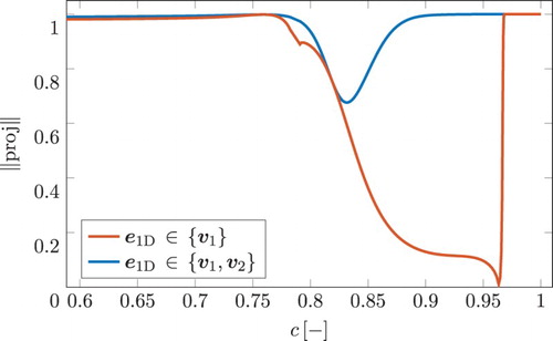It can be observed that Equation (10(10) ) holds for c>0.97, where the magnitude of the projection is equal to 1. For a slightly lower value of c, the direction of the 1D FGM lies in the surface locally spanned by the two slowest eigenvectors, such that it additionally includes the direction of the second eigenvector, attaining an even more significant component in the direction of the CO-related chemistry. Therefore, the unit vector tangent to the direction of the 1D FGM can be written as a linear combination of the two slowest eigenvectors, giving (11) where and are linear coefficients. This would mean that the length of the projection of on the plane , spanned by the two eigenvectors, is equal to 1. For the flamelet considered here, Equation (11(11) ) holds for c>0.9, as can be observed by looking at the blue line in Figure 2. For the part of the flamelet with c<0.9, resides in the planes spanned by a higher number of eigenvectors than the two slowest ones. Consequently, local flat planes formed by the two eigenvectors are not completely aligned with the direction of the 1D FGM; instead, the planes intersect the 1D FGM with an inclination angle and a significant component of is pointing out of the plane. For this part of the flamelet, the planes spanned by the two eigenvectors do not form a continuous manifold surface. This means that a 2D FGM-REDx cannot be constructed there, because the underlying assumption does not hold and actually a third reactive dimension is required to deal with this complication. Three or even more slowest eigenvectors can be utilised to obtain a manifold with a higher number of reactive dimensions. In this regard, it should be mentioned that the approach explained above can be extended to account for more chemical time-scales than only the two slowest ones. With an arbitrary number of chemical degrees of freedom given by , a multidimensional FGM-REDx can be constructed by utilising eigenvectors of the Jacobian matrix of the chemical source term, corresponding to the slowest chemical time-scales, . Then the manifold will be an -dimensional surface in composition space locally spanned by . Still, the adopted assumption here is that the perturbations in directions of the fastest reaction modes , with and , will reach steady-state infinitely fast. In practice, this approach may result in certain numerical complications, caused by the fact that for lower reaction progress, the reaction groups become intertwined and their time-scales cannot be separated (crossing of eigenvalues). This has been considered as one of the typical challenges in application of the time-scale analysis of the Jacobian of the source term, as reported, among others, by Eggels and de Goey [24].

Figure 1. A ribbon schematic representation of the 2D FGM-REDx for a part of the post-flame zone of a premixed flamelet. c-axis represents a scaled reaction progress variable. The remaining two axes show the mass fractions of CO and NO. The local directions of the eigenvectors and are shown, respectively, in red and yellow. Grey are projections to ease the visualisation. This figure is available in colour online.

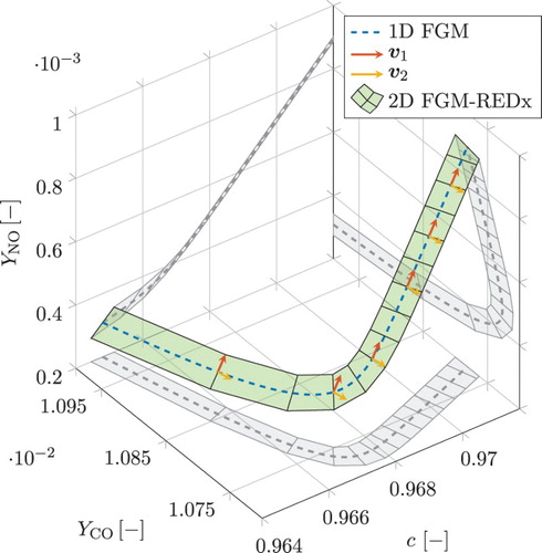
Figure 2. Magnitude of the projection of the unit vector tangent to the direction of the 1D FGM, , on the slowest eigenvector (red) and the plane spanned by the two slowest eigenvectors, (blue). This figure is available in colour online.

2.3. Parametrisation and tabulation of the FGM-REDx

In this section, the algorithm used for the generation of an FGM-REDx is presented. It is an example of an implementation strategy which can be used to apply the tabulated chemistry methods, such as FGM or ILDM. To illustrate this process with graphic examples, the flamelet from the previous section is further utilised.

2.3.1. Fundamental standard FGM

The FGM with one reactive dimension serves as a starting point for the generation of the FGM with REDx. Due to that, some aspects of the FGM with are briefly considered here first. It is described in detail in references [6] and [10]. To account for the effects of various physical processes, the manifold can include extra dimensions for a number of conserved control variables, such as mixture fraction, enthalpy and pressure. The presented method can be performed for every level of the conserved control variables of a particular standard FGM. For now, these variables are not considered, assuming them to be constant. Besides these additional conserved control variables, the manifold is parametrised by one reactive control variable, which is referred to as reaction progress variable, . It is defined as a linear combination of species mass fractions, being an inner product of the vectors of the linear coefficients, , and the mass fraction, , of species i, it is given by (12) The coefficients are constant throughout the entire manifold. These have to be chosen in such a way that the progress variable remains monotonic throughout the combustion process in order to allow for a valid parametrisation of the manifold. Further in this work, is used without additional normalisation. Thus, depending on the choice of the linear coefficients , progress variable does not necessarily need to range from zero to one, in counterpart to the scaled progress variable c.

2.3.2. Vectors locally spanning the FGM-REDx

When the 1D FGM has been generated, the following method is used to extend it with additional reactive dimensions. The FGM-REDx, with two or more reactive dimensions , is found by performing the eigenvalue analysis, explained in the previous Section 2.2, in each discrete point k of the 1D FGM. Then, the slowest eigenvectors are used to span the manifold locally: (13) where is a point in composition space residing on the dimensional FGM-REDx, is the composition of the original point k on the 1D FGM, and is a vector of linear coefficients with components. In the left graph of Figure 3 an example of Equation (13(13) ) is shown for one point k of the premixed flamelet. The path of the 1D FGM is shown by the blue dashed line, is given by the blue dot. The directions of the two slowest eigenvectors and in point k are shown in red and yellow. According to Equation (13(13) ), any feasible linear combination of these vectors added to forms a point in composition space that belongs to the local plane of the 2D FGM-REDx, which is shown in green.

Figure 3. On the left side, an example is shown of the flat plane locally forming a 2D FGM-REDx for one grid point k. The plot regards a post-flame part of a premixed flamelet. Axes represent the progress variable, , a secondary reactive control variable, , and the mass fraction of CO. The plot at the right, shows the tabulation grid for multiple grid points k on the 1D FGM in the plane of the two reactive control variables. This figure is available in colour online.

2.3.3. Strategy for tabulation of the FGM-REDx

In the particular implementation utilised in this work, the following strategy is used to facilitate a straightforward tabulation and lookup. The plane of the FGM-REDx with reactive dimensions, formed by the slowest eigenvectors, is spanned in a basis by new vectors. The first of these vectors is directed along the 1D FGM. This is only possible if the local direction of the 1D FGM resides in the plane spanned by the slowest eigenvectors. In general, this is not always the case, and extra dimensions might be required. The remaining vectors spanning the new basis are chosen to be orthogonal to the direction of the reaction progress variable. In other words, the composition of the points of the D FGM-REDx constructed locally in discrete point k of the 1D FGM will yield the values of the progress variable equal to that of . The implementation of the tabulation is not unique and various other strategies can be adopted. However, in this way, a structured table grid is created, allowing to first perform a table search in the dimension of the progress variable, followed by the search in the subsequent secondary reactive dimensions of the manifold. For the example of FGM-REDx with two reactive dimensions depicted at the left in Figure 3, the direction of the vector spanning the second dimension of the 2D manifold is shown by the blue arrow. It is further denoted as a linear combination , where and are linear coefficients. It can be observed that this line resides in the plane of the FGM-REDx as its direction is a linear combination of and . Additionally, as explained above, the linear coefficients and are chosen in such a way that the obtained linear combination is perpendicular to the -axis. This can be noticed from Figure 3, by observing that the blue vector and its projections have no component in the direction of .

2.3.4. Secondary chemically reactive control variables

Now, the direction of the extension is obtained and it can be stored in the table. This requires an additional step, which is determining the choice of the control variables. To parametrise the obtained dimensional manifold, additional control variables are necessary. Similarly to the reaction progress variable, these variables are chemically reactive, meaning that they describe the evolution of thermochemical state due to conversion of some species into others by chemical reactions. Further in this work, these are referred to as the secondary chemically reactive control variables , with , while the progress variable is the primary chemically reactive control variable. Similar to the progress variable, the secondary reactive control variables are defined as linear combinations of species mass fractions, with linear coefficients . The definition of all the chemically reactive control variables, that of the reaction progress variable and the secondary ones, is given by (14) which is a generalisation of Equation (12(12) ). Furthermore, the choice of the reactive control variables should result in a unique mapping of the obtained FGM-REDx on the control variable space. For the 2D FGM-REDx in the 3D plot in Figure 3, the choice of can be considered as suitable, because the plane of the 2D manifold has a nonsingular projection on the plane of the two reactive control variables. This projection is depicted in grey at the bottom coordinate plane of the drawing. The same holds for the vector , which should, and does in Figure 3, attain a non-zero -component. The values of the coefficients are not unique. On the contrary, these should be chosen to meet the above requirements for a particular flamelet database and are thus dependent on the mixture conditions. The values of utilised in this work will be discussed in Section 3.

2.3.5. Structured table grid

After the control variables are defined, a structured table grid is constructed for the reactive control variables . In the example of the 2D FGM-REDx given in Figure 3, for each point k, the additional reactive dimension of the manifold is stored by points in the table. The mid-point of this grid, l=2, tabulates the original FGM with one reactive dimension, attaining the value of the composition given by . The two remaining (peripheral) points, l=1 and l=3, parametrise the extension achieved by moving off the flamelet in the direction of the secondary reactive control variable . These two points are found by applying the magnitude of the extent of given by Δ, in, respectively, the negative and the positive directions. Theoretically, as the manifold is extended applying linear analysis around the 1D FGM, Δ should be chosen sufficiently small so that the extension remains in the direct vicinity of the 1D FGM. It can be verified that the magnitude of Δ is sufficiently small in order for the linear assumption to hold. This verification can be performed by conducting a Jacobian eigenvector analysis at the new obtained extended composition and comparing the hyperplanes spanned in composition space by the old slowest eigenvectors to the hyperplane spanned by the new ones. If the new set of eigenvectors lies in the hyperplane spanned by the original ones, it can be concluded that the extended manifold is satisfying the linear approximation, as the two hyperplanes are similar. In this work, due to practical considerations, Δ is assigned a value equal to the largest occurring deviation from the 1D FGM in the simulations of the utilised test cases described in Section 3. It also has been confirmed that the magnitude of Δ in this test cases still satisfies the linear assumption, as the verification procedure described above showed the occurring deviations to be less than . On the right side of Figure 3, a 2D plot is shown representing the plane of the two reactive control variables for the same region of the premixed flamelet shown on the 3D plot. Multiple grid points k in the 1D FGM are shown with blue dots. The two peripheral points l of the second reactive dimension are given by the purple dots for each grid point k. The extent of the second reactive dimension is taken to be . Together, all these points, k and l, form the table grid of the 2D FGM-REDx.

2.3.6. Algorithm for the implementation

This tabulation approach can be easily extended for more than two chemically reactive dimensions. Denoting the extend of the j'th FGM-REDx dimension by a multidimensional table grid of the control variables can be created by (15) where × and denote Cartesian product, which is a set of all possible combinations of the elements of vectors containing grid coordinates for each dimension. The resulting matrix has a size of by . Its first row corresponds to the progress variable and it is equal to the local progress variable value in the 1D FGM, . In the implementation utilised in this work, the task of Equation (15(15) ) is accomplished by calling a Matlab built-in function ndgrid.

The flow diagram in Figure 4 shows a schematic of the procedure employed for the generation of an FGM-REDx. As an input, this implementation receives the 1D FGM. After completing the generation for one level of conserved quantities, it can be repeated for the next one. In the particular approach utilised in this work, the loop over grid points k of the 1D FGM is iterated backwards starting from the equilibrium point of the original manifold, . This strategy is adopted, because the D FGM-REDx is defined in the best way in chemical equilibrium. This is substantiated by the fact that in chemical equilibrium all characteristic reaction groups are extinguishing () and their time-scales are usually well separated. In each k-iteration, after the computation of the eigenvectors, a check is performed if an FGM-REDx can be attained. This is done by verifying that the time-scales of the reaction groups being accounted for, with , are smaller than and well separated from the time-scales of the reaction groups assumed to be in steady state, with . In this work, an arbitrary tolerance for this difference is chosen to be equal to one percent. One special example of an insufficient time-scale separation is when complex values are attained for some of the slowest reaction groups , . In addition, the time-scales assumed in steady state have to be extinguishing, with , though in the test cases presented in this work, no positive eigenvalues were encountered in the parts of the 1D FGM where FGM-REDx could be attained. If, at a given point k of the 1D FGM, the separation of time-scales is insufficient, the process is terminated and the remaining part of the original 1D manifold, , will not be extended with additional reactive dimensions. During the CFD simulation for this part of the reaction progress, the 1D FGM is applied and the lookup is independent of the secondary reactive control variables. Eventually, to address a problem of variable number of tabulation cells, for this part of the reaction progress, all manifold extension cells may be filled with the local thermochemical composition on the 1D FGM.

Figure 4. Flow diagram illustrating the procedure of the generation and tabulation of the -dimensional FGM-REDx, conditioned for one level of conserved control variables.

As the next step of the flow diagram in Figure 4, for the point k of the 1D FGM the reactive control variables grid, with is defined. This tabulation grid is conditioned for the local level of reaction progress variable in grid point k, . Then for each point of the l-grid, the chemical composition vector has to be reconstructed, before it can be stored in the table. The chemical composition in grid point l can be found by utilising Equations (13(13) ) and (14(14) ). These equations are combined in the following linear system using matrix notation (16) which can be solved for knowing the matrix of the slowest eigenvectors , , the composition of the grid point k in the original 1D manifold , and with the linear coefficients matrix , , of the reactive control variables defined in the preceding steps. Further, vector , appearing in Equation (16(16) ), has components. After attaining the chemical species composition vector , the values of the related dependent thermochemical quantities are computed. Especially high importance is entailed in the computation of the reaction source terms of chemical species, . Though, can be computed as function of the species composition , enthalpy and pressure, in this work, a simplified approach is applied. The species reaction source terms is computed from the Jacobian matrix, equation (8(8) ), by (17) in which the deviations of species composition is assumed sufficiently small so that the source term changes linearly compared to its value in the 1D FGM, . The remaining dependent thermochemical quantities of interest, such as temperature and transport coefficients are computed as function of thermochemical composition vector in point l of the dimensional FGM-REDx, , taking the values for enthalpy and pressure from the point k in the 1D FGM.

3. Test case setup

3.1. Test case description

The performance of the newly developed FGM-REDx is examined in a test configuration simulating the process of expansion of a mixture of burnt gases. The purpose of this exercise is to create a situation where additional times scales of the reaction kinetics become important. This is achieved by applying a fast time-scale of expansion process to obtain conditions severe enough for the thermochemistry to leave the 1D FGM. The example considered here concerns the post-flame process arising in an aero-engine combustor. There, the burnt gases, formed in the combustor, are led through a decreasing area duct, causing the combustion heat to be converted into kinetic energy. This translates to an increase of velocity while temperature and pressure are decreasing. Inside this passage, called NGV, combustion products may accelerate up to almost the speed of sound. Due to that, the residence time inside the NGV is small, thus the cooling and the expansion are characterised by fast time-scales. These fast time-scales of the change of the thermodynamic variables interact with the post-flame chemistry, altering the concentration of the pollutants. The NGV test cases are nontrivial as the physics of varying enthalpy and pressure is absolutely absent in the utilised manifold flamelets, as those are computed at adiabatic and isobaric conditions.

3.2. Simulation setup

In the test cases utilised in this work, NGV conditions are mimicked in one-dimensional simulations. Considering only one spatial dimension has as advantage that a solution, using a detailed chemistry model, can be easily realised and applied for the validation of the FGM results.

The simulations are performed using the 1D laminar flame solver of Eindhoven University of Technology, CHEM1D [23] and the adopted detailed chemical mechanism is GRI-Mech 3.0 [22]. Also, unity Lewis numbers diffusion model is adopted, which is an acceptable simplification for methane flames, as the effective Lewis number is close to unity. Simulations utilising detailed reaction kinetics solve differential equations for continuity, species mass fractions and enthalpy, given by (18a) (18b) (18c) The surface area profile, , or in other words the geometry of the nozzle, is set in such a way that the Mach number, M, changes linearly in physical space: (19) with L, the length of the domain, inlet Mach number and the Mach number at the outlet of the domain . The profile for the surface area A is given by the following isentropic flow relation [25] (20) where represents the surface area scaled with its value at the inlet boundary and γ the ratio of specific heats. To avoid solving a momentum transport equation to obtain pressure, the profile for pressure is set as function of Mach number by utilising the isentropic flow relation (21) At the inlet, , a gas mixture with an equilibrium composition is flowing in, representing burnt gasses formed in the combustor. This composition corresponds to the chemical equilibrium of a stoichiometric methane-air mixture with the pressure and inlet enthalpy conditions equal to the values at the inlet of the nozzle. The pressure value at the inlet of the NGV is given by , while the inlet enthalpy, , is equal to that of stoichiometric methane-air mixture at an unburnt temperature of . These conditions roughly correspond to the inlet conditions of an airplane engine combustor and the overall drop in the enthalpy corresponds to of the enthalpy of combustion . To investigated how FGM accuracy is affected by the rate at which the enthalpy and the pressure change, a series of nozzle simulations have been performed varying the length of the domain, L. As a result, these test cases have different time-scales of expansion related to the residence time τ. In this series of computations, the residence time varies from (for ) up to (for ). 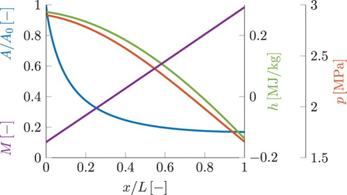For all computed cases, the lengths of the domain and the corresponding residence times are given in Table 2. Figure 5 shows the surface area, Mach number and the corresponding pressure and enthalpy plots for a one-dimensional simulation of a converging nozzle. The flow is from left to right. Mach number is increasing. The profiles for surface area A and pressure p are prescribed by Equations 20(20) and (21(21) ), implicitly assuming a linear increase of Mach number. The enthalpy and the Mach number profiles are following from the simulation. The corresponding profile for enthalpy h is found solving a transport equation, which includes a sink term due to negative pressure gradient. The profile for Mach number shown in Figure 5 is postprocessed from the simulation results and as can be observed, it resembles the implicitly prescribed profile given by Equation (19(19) ).

Table 2. Domain length L and the corresponding residence time τ for the series of the examined nozzle simulations.

Case number	1	2	3	4	5	6	7
	5	25	50	100	200	400	500
	0.13	0.66	1.3	2.6	5.3	11	13

Figure 5. Profiles of the surface area, Mach number, enthalpy and pressure in the NGV simulation.

3.3. Configuration of the FGM's

The following configuration is utilised for the generation of the 1D FGM and the 2D FGM-REDx, in the context of the test cases described above. The 2D manifold utilises the same configuration as the 1D FGM, differing only in the number of chemically reactive dimensions. The FGMs are generated from stoichiometric freely propagating premixed laminar methane-air flamelets computed at constant pressure and adiabatic conditions. Since enthalpy and pressure are changing in the nozzle simulations, their variation is incuded in the manifolds by two additional conserved control variables. In order for the FGM to be applied in the test cases mimicking a nozzle, flamelets are computed at various pressure and inlet enthalpy. The range of these parameters is chosen in a way to cover their range expected in the simulations and is given by (22) where the inlet enthalpy is specified in terms of the unburnt mixture temperature . The extents of pressure and inlet enthalpy are subdivided in, respectively, 10 and 20 equally spaced steps, and a flamelet is calculated for each combination, resulting in a flamelet database comprised of 200 flamelets. Subsequently, these flamelets are utilised to generate manifolds with pressure p, enthalpy h, as conserved control variables and one () or two (,) chemically reactive control variables. The coefficients and in the definitions of progress variable and the secondary reactive control variable are given in Table 3. The coefficients in the difinition of the reaction progress variable are found following the optimisation procedure of Niu et al. [26]. The definition of the secondary reactive control variable is as well optimised, utilising a method based on a similar concept. This is done in order to guarantee a unique parametrisation, in addition optimising for an improved interpolation accuracy. The optimisation of the control variables definitions is not necessary nor essential, it can be omitted simply using reactive control variables definitions found manually by trial and error. One of the crucial aspects is that the control variables should guarantee a correct parametrisation of the manifold. The optimisation procedure is utilised here as it is more convenient and results in a higher accuracy than choosing control variables manually. The same computations have been performed with another set of control variables definitions, which have been chosen by trial and error and similarly provided a correct parametrisation of the manifold. The obtained results are almost identical to those presented further in this work ; however, these are omitted here for brevity. It is worth noticing that, in general, different choices of the control variables definitions may lead to different results, especially if the perturbations from the manifold are large. Although, in the test simulations presented further in this work, this effect is minimal. Note that the definitions of the reactive control variables are based on only a small number of species with a large variation along the given manifold dimension, as this set was sufficient to provide a correct parametrisation. To aid the visualisation, a constant is added to to make it zero at the unburnt composition, . Further, the scaling of the coefficients vector is chosen in such a way that the maximum occurring chemical equilibrium value of is equal to unity. The manifold tabulation is performed on a curvilinear mesh. The table grid in p and h is equidistant and it is shown in Figure 6. This plot additionally indicates the local chemical equilibrium mass fraction of CO for each p and h combination. Further, the analytical curve of these two variables related to the expansion in the NGV simulation is depicted in red. The values of pressure and enthalpy are highest at the NGV inlet, decreasing in the process of expansion as the mixture is flowing through the converging nozzle. The table grid in progress variable, , is refined on the burnt side, as the computed test cases are close to conditions of chemical equilibrium. A rather high resolution in progress variable is chosen to avoid uncertainties due to interpolation inaccuracies, in order to focus the analysis on the aspects of the chemistry reduction methods. Note that during the manifold generation, for each flamelet, an extrapolation in progress variable space is performed to its super equilibrium values. In other words, the part of the manifold corresponding to the progress variable values higher than its chemical equilibrium value, , is found by performing a linear extrapolation and is stored in the table. The mesh of the second chemically reactive dimension is tabulated on an equidistant grid. Figure 7 illustrates the post-flame part of the obtained FGM-REDx, projected on the coordinate plane of the two reactive control variables. The plot regards the manifold conditioned for one pressure and enthalpy level given by and h corresponding to , other pressure and temperature levels are treated similarly. The colour bar indicates the mass fraction of CO. The lines represent the curvilinear mesh of and . 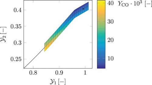It can be observed that for each point on the 1D FGM, the two table grid points of the extension are at the same level of the progress variable, reaching in the positive and the negative directions in the secondary reactive control variable relative to its local value on the original 1D manifold. The coordinate of the chemical equilibrium composition is given by the black dot. As can be seen from the figure, the manifold is extrapolated to super equilibrium values in progress variable space.

Table 3. Weights of chemical species in the definitions of the reactive control variables.

Species i
	20.439	0	1.941	0.002	2.311	0	0	1.928	9.049	0
	0.907	1.798	1.355	0.773	1.434	0.541	0.176	1.688	4.269	23.888

are the linear coefficients in the definition of ; are the coefficients in the definition of . for all species i not listed in the table.

Figure 6. Tabulation grid for pressure (p) and enthalpy (h). Colour shows the local chemical equilibrium values for the mass fraction of CO. The red line shows the pressure and enthalpy curve of the expansion in an NGV simulation (from high pressure and enthalpy values to the low ones). This figure is available in colour online.

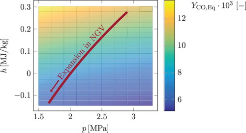
Figure 7. Schematic representation of the 2D FGM-REDx table grid of the two reactive control variables. Here the manifold is conditioned for one pressure and enthalpy level ( and h corresponds to ). The colour bar indicates the local CO mass fraction. The local chemical equilibrium point is given by the black dot. This figure is available in colour online.

The set of equations solved applying the manifold in a nozzle simulation is similar to that solved in case of detailed chemistry, except that of the equations for chemical species. FGM simulations presented in the following section, utilise Equations (18a(18a) ), (18c(18c) ) and (21(21) ), besides solving transport equation(s) for one or two reactive control variables: (23) At runtime, the source terms and the transport coefficients λ and are supplied by table lookup (using a linear interpolation). This, in conjunction with the number of solved differential equations being reduced by one order of magnitude and the stiffness being removed, results in roughly two orders of magnitude lower simulation times compared to those of the detailed chemical model.

4. Results

In this section, the performance of the FGM-REDx model is compared to that of a traditional 1D FGM. Detailed chemistry simulations (DC) are used as a reference for the assessment of the results found with the reduced chemistry.

4.1. Detailed chemistry results

In Figure 8 the detailed chemistry results are shown for the mass fractions of CO and NO for multiple mimicked nozzle simulations. The domain length L varies between and , corresponding to residence time τ from to , as listed in Table 3. For both species, the curves with the maximum values correspond to the shortest residence time. The values decrease as the residence time increases. It is worth noting, that the local chemical equilibrium values of all thermochemical variables are not constant throughout the domain. This is because the thermodynamic properties (h and p) are changing in space and . Due to almost similar pressure and enthalpy profiles as function of the normalised x-coordinate, the simulations share similar chemical equilibrium curves in normalised physical space. Because of decreasing temperature and pressure, the local chemical equilibrium values for both CO and NO are declining. For the case with the smallest residence time, the CO mass fraction decreases but not as much as the local chemical equilibrium. As a result of fast cooling, CO cannot follow the local chemical equilibrium. As the residence time becomes larger, CO is approaching the local chemical equilibrium. Similar trend is seen for the mass fraction of NO. However, due to the slower time-scale of NO chemistry, its relaxation to the local chemical equilibrium proceeds slower than that of the CO. This is especially pronounced for the simulation with the smallest residence time, where NO change is negligible, yielding outlet concentrations only a fraction smaller than the inlet value. With increasing residence time, there is a noticeable reduction of the NO mass fraction, nevertheless it remains above the equilibrium curve even in the simulation with the largest residence time. It can be assumed that for an infinite residence time all thermochemical variables would follow local chemical equilibrium.

Figure 8. Detailed chemistry results (solid lines) and local chemical equilibrium (dashed line) for the mass fractions of CO and NO for various lengths of the domain: (corresponding to different residence times).

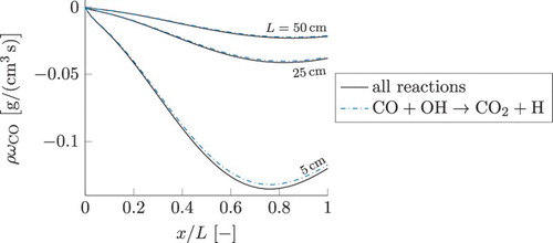
The decrease of is, for more than , caused by one chemical reaction. Its reaction equation is given by (24) The component of this reaction in the total source term of CO is shown in Figure 9 by a blue dashdotted line (for three smallest residence times τ discussed previously). For comparison, the total source term of CO is plotted by the solid line. Curves with the highest magnitude correspond to the smallest residence time, the magnitude decreases as the residence time becomes larger. As can be observed, the profiles of the source term due to this reaction are almost identical to the total source term of CO. In line with the results for in Figure 8, as its concentration approaches local chemical equilibrium, with increasing residence time τ, the magnitude of its sink term is decreasing.

Figure 9. Reaction source term of CO for the three test simulations with the smallest residence times. Solid line represents the total source term. The values obtained considering only one chemical reaction, , are given by the blue dashdotted line. This Figure is available in colour online.

In Figure 10, the detailed chemistry results are shown for the source terms of the local values of the two slowest eigenvectors and . These are postprocessed by taking the inner product of the corresponding left eigenvectors, , and the local source term vector . The orientation of is taken to yield a positive NO component. In case of , the sign of component is chosen to be positive, which results in a negative CO source component. For this analysis, are used in terms of specific mole numbers. For both eigenvectors, the curve with the largest magnitude corresponds to the simulation with the smallest residence time. For the remaining six simulations, the source term magnitude is decreasing with incrementally increasing residence time. As explained earlier, for the presented series of calculations varying the length of the domain, the compositions gradually attain values closer to local equilibrium, consequently yielding smaller reaction rates. Table 1 contains approximate values of these reaction groups. The slowest eigenvector , has a large positive NO component which is coupled with minor conversion of to CO. According to the figure, the source term of yields negative values, indicating a reduction of NO and CO accompanied by formation of (and oxygen). The second slowest eigenvector has a large negative CO component and a positive component with the same magnitude. The source term of in Figure 10 is positive expressing reduction of CO. As can be observed, has a magnitude of the source term which is two orders of magnitude smaller than that of . This can be explained by their respective time-scales (eigenvalues), given by and , these are separated by two orders of magnitude. The two following (faster) reaction groups and yield source terms (not shown here) with a negligible magnitude in the order of , with . It can thus be concluded that the perturbation of the chemical composition in the presented test cases mainly occurs in the directions of the two slowest eigenvectors.

Figure 10. Chemical source terms of the local values of the two slowest eigenvectors and postprocessed from the detailed chemistry simulation by taking an inner product of the species chemical source terms vector, and the corresponding left eigenvector . The source term magnitude is decreasing with incrementally increasing length of the domain L.

4.2. Standard FGM results

Moving to the FGM predictions, first the results obtained with 1D FGM are presented and discussed. To conduct a preliminary verification of the FGM, the values of the control variables have been reconstructed from the detailed chemistry results and these have been used to perform table lookup of the dependent quantities. The obtained profiles for the dependent quantities are then compared to their values in the detailed chemistry simulations. This procedure is further referred to as a priori FGM analysis. On the other hand, results obtained by applying the manifolds in actual simulations, solving Equations (18a(18a) ), (18c(18c) ) and (23(23) ), are further referred to as a posteriori FGM results. Figure 11 shows a priori FGM results for pollutants. The two subplots at the top correspond to the test case with the smallest residence time, , while the two at the bottom show the results for the largest residence time with . For both cases, 1D FGM predicts the mass fraction of CO to be very close to local chemical equilibrium, which is not in agreement with detailed chemistry results for the shortest residence time. In counterpart, for the longest residence time, where DC CO prediction follows local chemical equilibrium, similar FGM results turn out to yield a good agreement with DC. For the mass fraction of NO a priori 1D FGM results yield an underprediction for the smallest residence time, while for the largest residence time, a good agreement with DC is obtained. Other species show similar results, but only the profiles for CO and NO are presented here for the reasons of brevity and because our primary focus is prediction of pollutants. Another dependent quantity of interest to be considered in the a priori FGM analysis is the source term of the reaction progress variable, . Obtaining a correct value for is a crucial aspect for overall accuracy of the FGM simulations, as the remaining quantities strongly depend on progress variable. Figure 12 shows a priori FGM results for progress variable source term, at the left for the test case with the smallest residence time and at the right for the largest one. As can be observed, 1D FGM is not capable of predicting the correct sign of the source term even when the detailed chemistry values for the control variables are supplied. Due to this reason, deteriorated results of the actual a posteriori, FGM simulations can be anticipated.

Figure 11. A priori FGM results for CO and NO. The two graphs on top correspond to the simulation case with the shortest residence time, the two at the bottom show the longest residence time case. The line styles for the results of the detailed chemical model (DC), local chemical equilibrium (Eq), the 1D FGM and the FGM-REDx are given in the legend. This figure is available in colour online.

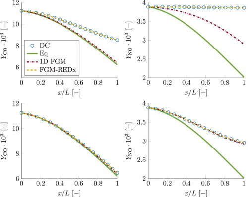
Figure 12. a priori FGM lookup for chemical source term of reaction progress variable. At the left plot simulation results are shown for the smallest residence time case, results shown at the right represent the simulation with the largest residence time. Legend for chemical models is similar to that in Figure 11. This figure is available in colour online.

Results for reaction progress variable, , obtained using different chemistry models, are shown in Figure 13, for the smallest τ (left) and the largest τ (right). In case of detailed chemistry, the shown values for progress variable are reconstructed from the species composition. The local chemical equilibrium value for progress variable is increasing as the gas mixture is flowing through the domain. The detailed chemistry curves show that the progress variable is increasing from the local chemical equilibrium at the inlet to the values above local equilibrium at the outlet. Its increase beyond the local chemical equilibrium is mainly associated with the NO mass fraction () remaining far above its local chemical equilibrium due to a slow time-scale of its evolution, as shown in Figure 11. In addition, part of the 1D FGM close to chemical equilibrium, , evolves solely along the slowest reaction group . There, in the 1D FGM case, all the progress along the faster reaction groups, including , has already reached partial equilibrium. This clarifies the a priori 1D FGM results for mass fraction of CO, in the smallest residence time simulation in Figure 11, being much closer to the local equilibrium curve than the detailed chemistry prediction, as has a smaller CO component. This in turn influences the 1D FGM predictions for the source terms of species in definition of progress variable, resulting in underpredicted magnitudes of . The fact that the a priori source term of progress variable in Figure 12, yields incorrect negative sign for 1D FGM, is explained by the DC progress variable curve in Figure 13 being above its local chemical equilibrium. In this way, the looked up values correspond to the region of the manifold obtained by extrapolation to super equilibrium, where its source term is negative. The FGM results for progress variable shown in Figure 13 are obtained by a posteriori FGM analysis (applying the manifolds in real simulations as explained earlier). For 1D FGM, the predictions for progress variable are underestimated and remain below the equilibrium curve. This is a direct consequence of the underpredicted source term of progress variable.

Figure 13. Simulation results for reaction progress variable, . Plot on the left represents the smallest residence time case, the one at the right represent the case with the largest residence time. Legend is similar to that in Figure 11. For 1D FGM and FGM-REDx, a posteriori results are shown. This figure is available in colour online.

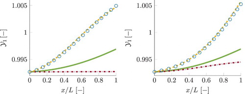
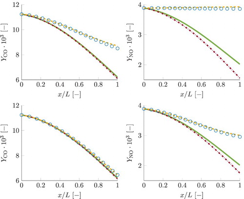
Figure 14 shows a posteriori FGM results for mass fractions of pollutants CO and NO. These are obtained by manifold lookup as function of the transported values for the control variables. As can be observed, the 1D FGM predicts curves for pollutants lying on the incorrect side relative to the local chemical equilibrium curves. This is a direct consequence of underpredicted simulation results for progress variable, shown in Figure 13. FGM results for the remaining control variables, pressure and enthalpy, showed only insignificant discrepancies with the detailed chemistry simulations and are therefore omitted.

Figure 14. Simulation results for mass fractions of CO and NO. Line styles for different chemical models are given in the legend of Figure 11. The two subplots at the top correspond to the smallest residence time case, while the two at the bottom correspond to the case with the largest τ. This figure is available in colour online.

4.3. FGM-REDx results

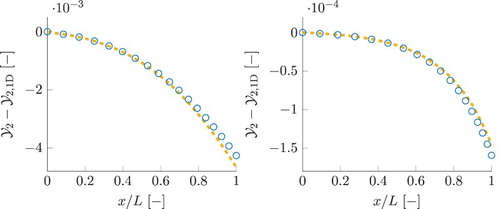
The newly developed FGM-REDx has been employed to perform simulations of the same test cases. The obtained results will now be discussed and compared to those obtained with 1D FGM, using detailed chemistry simulations as reference. The first question arising regards the importance of the second chemically reactive dimension of the FGM. This can be analysed considering the magnitude in which the composition deviates from the 1D FGM in the direction of the extension. The surplus of the secondary reactive control variable, , compared to its local value in the 1D FGM, , is shown in Figure 15. As can be observed, DC values for the case with the smallest τ (left subplot) are one magnitude larger than those of the case with the largest τ (right subplot). Thus, the level of how much the thermochemistry is going off the 1D FGM is inversely proportional to the time-scale of the change of thermodynamic variables. The FGM-REDx curves regard the a posteriori results, obtained in actual FGM simulations. The FGM-REDx shows a very good agreement with detailed chemistry for the second reactive control variable. Also, looking back at the plot for progress variable, Figure 13, it can be observed that the FGM-REDx yields a very good prediction for . 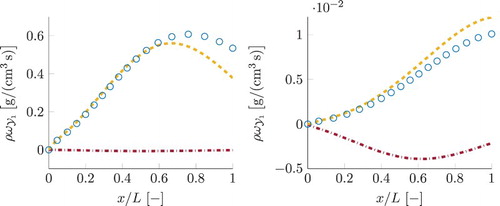Although, the quantitative agreement is not perfect for the source terms of progress variable, , shown in Figure 12. This is a consequence of a linear approximation of the chemical source terms along the secondary reactive dimension. The minor deviations from the detailed chemistry curves indicate that the higher order terms become important, as the reaction rates are non-linear functions of the species composition. Further, the FGM-REDx results for the pollutants in Figure 14 show a good agreement with detailed chemistry. It can be concluded that including an additional reactive dimension results in a much better representation of the thermochemical composition. As a consequence, the reaction source terms of the control variables are predicted with an improved accuracy resulting in a good agreement for control variables. In turn the pollutants mass fractions yield correct values in the 2D manifold when looked up as a function of the well predicted control variables.

Figure 15. Surplus of the secondary reactive control variable, , compared to its local value in the 1D FGM, . Detailed chemistry and FGM-REDx simulation results are shown using similar line styles as in Figure 11. Results for the case with the smallest τ are shown in the left subplot, the profiles for the case with the largest τ are shown in the right subplot. This figure is avaialble in colour online.

In 2D FGM-REDx a finite rate chemistry of reactions is taken into account in addition to that of . In this way, CO and can relax towards the local chemical equilibrium concentrations considering a finite rate of the evolution along this reaction group. For example, chemical reaction in Figure 9 has, consequently, a finite rate, as the reactants CO and OH are not considered to be that close to local chemical equilibrium. Allowing for an additional time-scale of chemical kinetics, also influences the NO predictions, as its rates and concentrations are coupled with the remaining species composition. An example of such two-way coupling are the CO and components in both slowest eigenvector, indicating that a correct representation of these species facilitates NO accuracy, and vice versa.

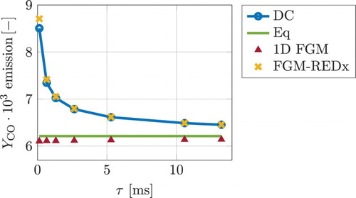
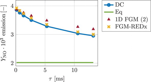
Figure 16 shows the CO values at the exhaust of multiple nozzle simulations plotted here against the residence time τ. The CO exhaust mass fraction comes closer to the local chemical equilibrium as the residence time increases. FGM-REDx is able to reproduce the detailed chemistry CO results, in counterpart to the 1D FGM.

Figure 16. FGM predictions for CO emissions for multiple simulations plotted as function of the residence time τ. Line styles for detailed chemistry (DC), chemical equilibrium (Eq), 1D FGM and FGM-REDx are given in the legend. This figure is avaialble in colour online.

5. NO modelling with additional transport equation

This section compares the current approach with various conventional NO modelling approaches applied in the context of reduced chemistry. These methods are based on solving an additional transport equation for NO, which is decoupled from the remaining thermochemical composition. The underlying theory is summarised in Section 5.1, followed by Section 5.2 presenting the results for transported NO applied in 1D FGM simulations of a nozzle test case. The 1D FGM transported NO results are then compared to the results obtained by the newly developed FGM-REDx approach utilising the simulations presented in Section 4.

5.1. Transported NO source term modelling methods

This section contains a summary of NO modelling techniques solving an additional transport equation, applied in the context of tabulated chemistry. These methods are succeeding steps of increasing complexity compared to the direct lookup of the NO mass fraction from the manifold as function of the control variables, as applied in Section 4. The transport equation for the mass fraction of NO in one physical dimension, under steady state and unity Lewis number assumptions, is given by (25) where is the reaction source term. The first method for modelling of the NO source term [16,17] is looking it up from the manifold: (26) A physical implication of this method is that by solving a transport equation for NO, it is allowed to attain a perturbation with respect to its value in the FGM. In this case, by analogy with the FGM-REDx, the species composition obtained by the reduced chemical model is then described by a vector locally extending the 1D FGM. However, NO is the only component of this direction and the evolution along this extension does not conserve the mass of the mixture, nor does it affect the composition of the remaining species and the reaction source terms.

The second method is solving a transport equation for NO utilising a more complex treatment for the source term . It includes a feedback of the local NO mass fraction as found by Equation (25(25) ) on the chemical source term of NO. This is achieved by correcting the rates of the consumption reactions of NO. Depending on if is larger or smaller than the value in the manifold , the rates of the consumption reactions are, respectively, increased or decreased. This results in a chemical source term attracting back to the manifold, introducing an additional time-scale of NO formation. This method was introduced by Ihme and Pitsch [18], and it is based on the observation that the rates of most NO consumption reactions are linear in the concentration of NO. In that case, the total source term can be decomposed as follows (27) into a contribution of a chosen set of consumption reactions, , and the remaining part of the NO source term, . Reminding that the stoichiometric coefficient of NO in most consumption reactions is equal to unity, the source term in transport Equation (25(25) ) is computed according to (28) with and being stored in the manifold. In the following section, an investigation is made of the effect of the choice of the set of the reactions which are considered to be dependent on NO mass fraction. Namely, a comparison is made between correcting the rates of only the three thermal NO consumption reactions, , and correcting all the NO consumption rates including also the prompt reactions, . Utilising this advanced model for the source term, the additional quasi-dimension of the FGM, with only non-zero component being the mass fraction of NO, receives a slightly higher influence on the solution, by including a variation of the NO formation rate. Still, it is not coupled back with the remaining thermochemistry.

Pecquery et al. [20] also solve a transport equation for NO mass fraction, in particular, it is used as a 1D FGM control variable in the NO relevant post-flame zone. In their work, the ILDM analysis has been applied to come to a conclusion that the mass fraction of NO is the best parametrisation option for burnt gases chemistry. However, the assumption has been used that the system evolves along the 1D manifold. Regardless of the parametrisation, the relaxation towards the 1D FGM is assumed to be faster than other perturbations, such as air dilution, restricting the evolution of the composition to one local chemical time-scale.

5.2. Transported NO results

In this section, the results for the mass fraction of NO are presented and discussed, investigating the relative performance of various reduced modelling approaches as explained in Section 5.1. The nozzle case utilised here has a domain length of . In this way, the residence time τ becomes in the order of . This is done because of the slow time-scale of the formation of NO, as for the shorter residence times the change of NO mass fraction inside the domain becomes negligible. Figure 17 gives the NO results found by applying various reduced modelling approaches in addition to the detailed chemistry curve, which is used as the reference. The mass fraction is shown in the left subplot and the predicted reaction source term is given in the right. As discussed in Section 4, the local chemical equilibrium curve is decreasing, which is caused by the decreasing enthalpy and temperature. The detailed chemistry model predicts that NO will decline in response to the equilibrium shift. However, due to the slow rate of its chemistry, NO cannot follow the equilibrium and remains above it. Further, in Figure 17, the results are shown for two reduced modeling techniques used here in the context of the 1D FGM. The dashdotted red line represents the results found by the direct lookup in the manifold as function of the control variables. The direct lookup of NO predicts a curve lying just below the local equilibrium. This is in a qualitative disagreement with the detailed chemistry. As explained in Section 4, it is caused by the fact that the composition in the given case does not reside in the manifold with one reactive dimension. This issue is subsequently amplified by inaccuracies in the progress variable. In more detail, 1D FGM predicts that the progress variable has values below the local equilibrium, while the detailed chemistry model yields super equilibrium values of . This is, again, one of the main reasons the direct lookup of NO predicts a curve lying just below the local equilibrium. The dash dotted purple lines, in the same figures, show the outcome of solving a transport equation for NO in the context of the 1D FGM. The first of these, indicated by the diamonds (labeled ‘’), is obtained reading the source term directly from the manifold as function of the control variables. The NO source term turns out to have a small positive value. The positive sign of the source term does not agree with the detailed chemistry. This is again because the reaction progress variable is underpredicted to be just below the local chemical equilibrium. At this location in the flamelet, the NO mass fraction continues to grow towards its equilibrium value and the 1D FGM will thus predict a positive source term. This does not agree with the detailed chemistry results.

Figure 17. Results for the NO mass fraction (left) and the chemical source term (right) found applying various reduced modelling approaches. Detailed chemistry curve is used as the reference. Line styles representing detailed chemistry, local chemical equilibrium and the direct lookup values from the 1D FGM and the FGM-REDx are given in the legend of Figure 11. Purple lines show the 1D FGM results obtained by an additional NO transport equation, utilising various approaches for the source term modelling. Their corresponding line styles are given in the legend. This figure is available in colour online.

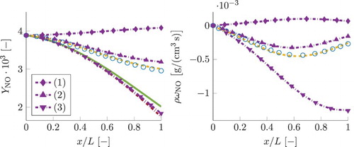
The remaining two purple curves represent the reduced models solving a transport equation for NO, letting its source term depend not only on the control variables, but also on the values of the NO mass fraction. As explained in Section 5.1, the source term adjusts so that NO is attracted back to its values in the manifold with a time-scale given by . The first of these, shown by the triangles pointing up (‘’ in the legend), applies this correction only to the consumption rates of the three thermal NO reactions, leaving the rates of the remaining production and consumption reactions equal to their manifold values. This model predicts a correct sign of the source term and the obtained results come closer to those of the detailed chemistry. Apparently, correcting only the thermal consumption reactions yields a correct time-scale of the relaxation of the NO back to the manifold. The second model configuration, denoted by triangles pointing down (labeled ‘’), shows the results of the model correcting all the reactions that consume NO. In this way, the relaxation of NO back to its manifold values would be much higher in comparison to the case enhancing only the three thermal consumption reactions. The consequence can be observed in the figure: this model yields a curve lying nearly on top of the one obtained by the 1D FGM direct lookup. Evidently, the amplification of all consumption reactions results in NO mass fraction being driven back to the manifold with an overestimated rate. In contrast to transported NO, results obtained by direct lookup utilising FGM-REDx, which has been presented in Section 4, show a much better agreement with detailed chemistry. This is explained by the fact, that including a full additional manifold dimension results in a coupling among the complete thermochemical composition compared to a quasi-dimension that yields an extra time-scale only for NO formation.

Figure 18 shows the exhaust values of the NO mass fraction for different nozzle domain lengths as function of the residence time τ. The two reduced models shown in Figure 18 are the (1D FGM) transported NO with the correction of the rates of the three thermal consumption reactions (model ‘’) and the direct lookup from the FGM-REDx. As can be observed, the relative improvement obtained with the FGM-REDx increases as the residence time becomes larger and the concentrations attain a significant variation compared to the (fixed) inlet value. Note that for the smallest residence time, the NO concentration does not change due to its slow chemistry, resulting in equal values at the inlet and the exhaust, which is predicted by both reduced models. The fact that the 1D FGM prediction for the exhaust NO is slightly (barely noticeable) better for the smallest τ case can be related to the numerical (lookup, etc.) inaccuracies arising due to the small relative variation of the NO mass fraction.

Figure 18. Values for the mass fraction of NO at the exhaust of multiple nozzle simulations with a varied domain length. Horizontal axis represents the residence time τ for each simulation. This figure is available in colour online.

6. Conclusions

A new method to extend the FGM with additional chemical time-scales, FGM-REDx, has been developed with the intention to improve the general accuracy of the representation of the reaction kinetics.

Additional chemically reactive dimensions were added to the manifold by analysing the time-scales of the chemical processes close to the 1D FGM. The slowest chemical processes were added as additional degrees of freedom while the faster ones are assumed in steady state. In this way, a higher-dimensional manifold can be constructed in the neighborhood of the 1D FGM. This approach is not necessarily restricted to one additional dimension. On the contrary, an arbitrary number of chemically reactive dimensions can be included. Additional transport equations are solved for extra chemically reactive control variables used to parametrise the movement in the direction of the extension. These control variables, similarly to the reaction progress variable, describe the evolution of the composition due to chemical reactions. Their definitions and transport equations are also analogous to those of the reaction progress variable. The tabulation of the higher dimensional manifold is performed using a structured table grid of the reactive control variables, though the implementation of the tabulation is not unique and various other strategies can be adopted.

The performance of the new developed model is examined in one-dimensional simulations of the process of expansion of a mixture of burnt gases in an aero-engine stator. The main focus was on the capability of the FGMs to predict the effects of the fast time-scale of cooling and expansion on the post-flame chemistry of pollutants CO and NO. As appeared from the detailed chemistry simulations, these high cooling rates result in a fast time-scale of the change of the local chemical equilibrium composition, which alters the concentration of the pollutants. Both CO and NO are not able to follow the decreasing local chemical equilibrium due to the slower time-scales of their chemistry, which results in higher pollutants emissions. The examined test cases showed that a 2D FGM-REDx yielded a higher accuracy compared to that of a traditional 1D FGM. The FGM-REDx was capable of quantitatively reproducing the results of the detailed chemistry model, while the 1D FGM was showing qualitatively different results. The NO predictions of the current approach also have been compared to those of the various conventional NO modelling methods applied in the context of reduced chemistry. These are based on solving an additional transport equation for NO. Three different methods for modelling of the chemical source term in the NO transport equation where investigated. It has been shown that, in the context of the 1D FGM, an acceptable level of accuracy is obtained by the method correcting the rates of the thermal NO consumption reactions as a linear function of the NO mass fraction. The new developed FGM-REDx model yielded either comparable or better NO predictions. This is attributed to the fact that its additional degree of freedom comprises all components of the thermochemical composition vector, as opposed to the transported NO methods, where the additional degree of freedom is restricted to the NO component, missing a coupling with the remaining thermochemistry and violating the conservation of mass. An evident advantage of a full coupling in case of the FGM-REDx is the accurate prediction of CO (and other species) in addition to that of NO. For the remaining transported NO models, it has been observed that reading the source term from the manifold without a dependency on NO, yielded an incorrect sign of the source term, while correcting all the NO consumption rates (including prompt reactions) resulted in NO mass fraction being driven back to the manifold with an overestimated rate.

In practice, a weak separation of time-scales of reaction kinetics (crossing of eigenvalues) may cause larger deviations, which has been considered as a typical challenge in the application of the time-scale analysis of the chemical source term.

In this work, it has been systematically demonstrated, that for the conditions where the rates of physical/thermodynamic perturbations are severe enough for the thermochemical composition to go off the flamelet, the FGM method can be successfully extended by including extra time-scales of chemical kinetics as additional FGM dimensions. In this way, a finite rate of the relaxation towards the (slower) 1D FGM is taken into account, resulting in a largely improved accuracy.

Disclosure statement

No potential conflict of interest was reported by the authors.

ORCID

Denis V. Efimov  http://orcid.org/0000-0002-2875-2146

Philip de Goey  http://orcid.org/0000-0001-6625-3113

Jeroen A. van Oijen  http://orcid.org/0000-0002-4283-2898

Additional information

Funding

The authors thank European Union's Seventh Framework Programme (FP7/2007-2013) for the Clean Sky Joint Technology Initiative under project DREAMCODE grant 620143 for supporting this research.

References

- U. Maas and S.B. Pope, Simplifying chemical kinetics: Intrinsic Low-Dimensional Manifolds in composition space, Combust. Flame 88 (1992), pp. 239–264. doi: 10.1016/0010-2180(92)90034-M
- U. Maas and S.B. Pope, Implementation of simplified chemical kinetics based on Intrinsic Low-Dimensional Manifolds, Proc. Combust. Inst., 24 (1992), pp. 103–112. doi: 10.1016/S0082-0784(06)80017-2
- V. Bykov and U. Maas, The extension of the ILDM concept to reaction-diffusion manifolds, Combust. Theory Model. 11 (2007), pp. 839–862. doi: 10.1080/13647830701242531
- N. Peters, Laminar diffusion flamelet models in non-premixed turbulent combustion, Prog. Energy. Combust. Sci. 10 (1984), pp. 319–339. doi: 10.1016/0360-1285(84)90114-X
- N. Peters, Laminar flamelet concepts in turbulent combustion, Twenty-First Symposium (International) on Combustion, 1986.
- J.A. van Oijen and L.P.H. de Goey, Modelling of premixed laminar flames using Flamelet-Generated Manifolds, Combust. Sci. Technol. 161 (2000), pp. 113–137. doi: 10.1080/00102200008935814
- O. Gicquel, N. Darabiha, and D. Thévenin, Laminar premixed hydrogen/air counterflow flame simulations using flame prolongation of ILDM with differential diffusion, Proc. Combust. Inst. 28 (2000), pp. 1901–1908. doi: 10.1016/S0082-0784(00)80594-9
- C.D. Pierce and P. Moin, Progress-variable approach for large-eddy simulation of non-premixed turbulent combustion, J. Fluid Mech. 504 (2004), pp. 73–97. doi: 10.1017/S0022112004008213
- M. Ihme, C.M. Cha, and H. Pitsch, Prediction of local extinction and re-ignition effects in non-premixed turbulent combustion using a flamelet/progress variable approach, Proc. Combust. Inst. 30 (2005), pp. 793–800. doi: 10.1016/j.proci.2004.08.260
- J.A. van Oijen, F.A. Lammers, and L.P.H. de Goey, Modeling of complex premixed burner systems by using flamelet-generated manifolds, Combust. Flame 127(3) (2001), pp. 2124–2134. doi: 10.1016/S0010-2180(01)00316-9
- S. Delhaye, L.M.T. Somers, J.A. van Oijen, and L.P.H. de Goey, Incorporating unsteady flow-effects beyond the extinction limit in flamelet-generated manifolds, Proc. Combust. Inst. 32 (2009), pp. 1051–1058. doi: 10.1016/j.proci.2008.06.111
- S.C. Hill and L.D. Smoot, Modeling of nitrogen oxides formation and destruction in combustion systems, Prog. Energy Combust. Sci. 26 (2000), pp. 417–458. doi: 10.1016/S0360-1285(00)00011-3
- F. Biagioli and F. Güthe, Effect of pressure and fuel-air unmixedness on NOx emissions from industrial gas turbine burners, Combust. Flame 151 (2007), pp. 274–288. doi: 10.1016/j.combustflame.2007.04.007
- A. Frassoldati, S. Frigerio, E. Colombo, F. Inzoli, and T. Faravelli, Determination of emissions from strong swirling confined flames with an integrated CFD-based procedure, Chem. Eng. Sci. 60 (2005), pp. 2851–2869. doi: 10.1016/j.ces.2004.12.038
- G. Godel, P. Domingo, and L. Vervisch, Tabulation of chemistry for large-eddy simulation of non-premixed turbulent flames, Proc. Combust. Inst. 32 (2009), pp. 1555–1561. doi: 10.1016/j.proci.2008.06.129
- W.P. Jones and C.H. Priddin, Predictions of the flow field and local gas composition in gas turbine combustors, Proc. Combust. Inst. 17 (1978), pp. 399–408. doi: 10.1016/S0082-0784(79)80041-7
- A.W. Vreman, B.A. Albrecht, J.A. van Oijen, L.P.H. de Goey, and R.J.M. Bastiaans, Premixed and nonpremixed generated manifolds in large-eddy simulation of Sandia flame D and F, Combust. Flame 153 (2008), pp. 394–416. doi: 10.1016/j.combustflame.2008.01.009
- M. Ihme and H. Pitsch, Modeling of radiation and nitric oxide formation in turbulent nonpremixed flames using a flamelet/progress variable formulation, Phys. Fluids 20 (2008), pp. 055110. doi: 10.1063/1.2911047
- A. Ketelheun, C. Olbricht, F. Hahn, and J. Janicka, NO prediction in turbulent flames using LES/FGM with additional transport equations, Proc. Combust. Inst. 33 (2011), pp. 2975–2982. doi: 10.1016/j.proci.2010.07.021
- F. Pecquery, V. Moureau, G. Lartigue, L. Vervisch, and A. Roux, Modelling nitrogen oxide emissions in turbulent flames with air dilution: Application to LES of a non-premixed jet-flame, Combust. Flame 161 (2014), pp. 496–509. doi: 10.1016/j.combustflame.2013.09.018
- J. Nafe and U. Maas, Modeling of NO formation based on ILDM reduced chemistry, Proc. Combust. Inst. 29 (2002), pp. 1379–1385. doi: 10.1016/S1540-7489(02)80169-9
- G.P. Smith, D.M. Golden, M. Frenklach, N.W. Moriarty, B. Eiteneer, M. Goldenberg, C.T. Bowman, R.K. Hanson, S. Song, W.C. Gardiner, V.V. Lissianski, and Z. Qin. GRI-Mech 3.0. Available at http://www.me.berkeley.edu/gri_mech/, 2000.
- Eindhoven University of Technology. CHEM1D. Available at www.combustion.tue.nl.
- R.L.G.M. Eggels and L.P.H. de Goey, Mathematically reduced reaction mechanisms applied to adiabatic flat hydrogen/air flames, Combust. Flame 100 (1995), pp. 559–570. doi: 10.1016/0010-2180(94)00108-5
- R.D. Zucker and O. Biblarz, Fundamentals of Gas Dynamics, 2nd ed., John Wiley & Sons, Inc., Hoboken, NJ, 2002.
- Y. Niu, L. Vervisch, and P. Dinh Tao, An optimization-based approach to detailed chemistry tabulation: Automated progress variable definition, Combust. Flame 160 (2013), pp. 776–785. doi: 10.1016/j.combustflame.2012.11.015