A DNS assessment of linear relations between filtered reaction rate, flame surface density, and scalar dissipation rate in a weakly turbulent premixed flame

Abstract

Linear relations between (i) filtered reaction rate and filtered flame surface density (FSD) and (ii) filtered reaction rate and filtered scalar dissipation rate (SDR), which are widely used in Large Eddy Simulation (LES) research into premixed turbulent combustion, are examined by processing DNS data obtained from a statistically 1D planar flame under weakly turbulent conditions that are most favourable for the two approaches (flamelet combustion regime, single-step chemistry, equidiffusive mixture, adiabatic burner, and low Mach number). The analysis well supports the former approach provided that the filtered reaction rate is combined with filtered molecular transport term. In such a case, both the RANS and LES FSD approaches are based on local relations valid within weakly perturbed flamelets. Accordingly, simply recasting RANS expressions to a filtered form works well. On the contrary, while the FSD and SDR approaches appear to be basically similar at first glance, the analysis does not support the latter one, but shows that a ratio of the filtered reaction rate to the filtered SDR is strongly scattered within the studied flame brush, with its conditionally mean value varying significantly with Favre-filtered combustion progress variable. As argued in the paper, these limitations of the LES SDR approach stem from the fact that it is based on a relation valid after integration over weakly perturbed flamelets, but this relation does not hold locally within such flamelets. Consequently, when a sufficiently small filter is applied to instantaneous fields, the filter may contain only a part of the local flamelet, whereas the linear relation holds solely for the entire flamelet and may not hold within the filtered flamelet volume. Thus, the present study implies that straightforwardly recasting well-established RANS equations to a filtered form is a flawed approach if the equations are based on integral features of local burning.

Keywords:

• turbulent combustion
• flame surface density
• scalar dissipation rate
• DNS
• LES

1. Introduction

Large Eddy Simulation (LES) is widely accepted to be a powerful research tool capable for making substantial progress in applied studies of various important combustion phenomena such as, e.g. thermoacoustic instabilities in gas turbine burners [1,2]. Nevertheless, from purely fundamental perspective, a problem of modelling flame-turbulence interaction at small scales unresolved in a typical LES is far from being solved. With a few exceptions, most LES models of the influence of turbulence on premixed combustion originate from models developed and validated for Reynolds-Averaged Navier-Stokes (RANS) simulations, provided that (i) mean quantities addressed by the RANS models are substituted with filtered quantities relevant to the LES models and (ii) Germano identity [3] is eventually used to evaluate the LES model constant(s). As examples of recasting RANS equations to a filtered form, LESs that deal with a transport equation for a Flame Surface Density (FSD) or a Scalar Dissipation Rate (SDR) will be considered in the following.

The reader interested in detailed discussion of the FSD or SDR approach to modelling premixed turbulent combustion within the RANS framework is referred to review papers by Veynante and Vervisch [4] or by Chakraborty et al. [5], respectively. Here, we restrict ourselves to a very brief summary of the two approaches. They aim at closing the mean mass rate $\overline{W}$ of product creation as follows (1) $\overline{W}={\rho }_u{S}_L\overline{\mathrm{\Sigma }},$(1) (2) $\overline{W}=2\overline{\rho }\tilde{\chi }/\left(2c_m-1\right),$(2) respectively, where $\rho$ is the density, subscript u designates unburned gas, $S_L$ is the laminar flame speed, $\mathrm{\Sigma }$ is a FSD, e.g. $\mathrm{\Sigma }=|\mathrm{\nabla }c|$ [4], $\chi =D\mathrm{\nabla }c\cdot \mathrm{\nabla }c$ is a SDR, $c_m=\overline{cW}/\overline{W}$ is often assumed to be constant within a turbulent flame brush [5–7], $\overline{q}$ and $\tilde{q}=\overline{\rho q}/\overline{\rho }$ are the Reynolds and Favre-averaged values of a quantity $q$, with $q^{\mathrm{\prime }}\equiv q-\overline{q}$ and $q^{\mathrm{\prime \prime }}\equiv q-\tilde{q}$, respectively, $c$ is the combustion progress variable used to characterise the state of a mixture within a flame, and $D$ is the molecular diffusivity of $c$.

Equation (1) stems from an assumption that the influence of turbulence on premixed combustion may be reduced to wrinkling the flame-front surface by turbulent eddies, with the local rate of product creation per unit area of the front being simply equal to ${\rho }_u{S}_L$. Accordingly, the rate of product creation per an infinitesimal volume $dV$ is equal to $\overline{W}dV={\rho }_u{S}_{L}dA$, where the area $dA$ of the front within the volume is equal to $\overline{\mathrm{\Sigma }}dV$. Consequently, Equation (1) holds.

Alternatively, Equation (1) can be substantiated by considering the unperturbed (i.e. planar, 1D, and fully-developed) laminar premixed flame. In the coordinate framework attached to it, such a flame is modelled by the following transport equation (3) ${\rho }_u{S}_L\frac{\text{d}c}{\text{d}x}=\frac{\text{d}}{\text{d}x}\left(\rho D\frac{\text{d}c}{\text{d}x}\right)+W.$(3)

If we assume that premixed flames in a turbulent flow retain the structure of the unperturbed laminar flames, then, the following equality (4) $\mathrm{\nabla }\cdot \left(\rho D\mathrm{\nabla }c\right)+W={\rho }_u{S}_L|\mathrm{\nabla }c|$(4) holds within such inherently laminar flamelets, i.e. in volumes where $0<c<1$. Consequently, (5) $\mathrm{\nabla }\cdot \overline{\rho D\mathrm{\nabla }c}+\overline{W}={\rho }_u{S}_L\overline{\mathrm{\Sigma }}$(5)

Equation (5) is similar to Equation (1), but involves an extra molecular transport term, see the first term on the Left Hand Side (LHS). This term is often neglected in RANS simulations when compared to turbulent transport term $\mathrm{\nabla }\cdot \overline{\rho {\mathbf{\text{u}}}^{\mathrm{\prime \prime }}{c}^{\mathrm{\prime \prime }}}$ in the transport equation for the Favre-averaged combustion progress variable $\tilde{c}$.

Alternatively, Equation (5) can be substantiated by introducing a displacement speed $S_d$ as follows [4] (6) $\rho S_d|\mathrm{\nabla }c|\equiv \mathrm{\nabla }\cdot \left(\rho D\mathrm{\nabla }c\right)+W$(6) and averaging Equation (6) by assuming that either (i) $\rho S_d={\rho }_u{S}_L$ or (ii) $\overline{\rho S_d}={\rho }_u{S}_L$ and $\rho S_d$ does not correlate with the FSD. The approach can further be extended by invoking the theory of weakly stretched laminar premixed flames [8,9] to allow for a correlation between $S_d$ and $|\mathrm{\nabla }c|$, but such an extension of the approach is beyond the scope of the present paper.

Thus, all substantiations of Equation (1) or (5), addressed above, are heavily based on a hypothesis that premixed turbulent combustion occurs in the flamelet regime, i.e. fresh reactants and equilibrium combustion products are separated by a thin zone (called flamelet) that retains the structure of the unperturbed (or weakly perturbed) laminar premixed flame.

Equation (2) is also justified for the same flamelet regime. Bray [6,7] rigorously derived Equation (2) by invoking two simplifications. First, the probability of finding intermediate states of the reacting mixture (i.e. $0<c<1$) was assumed to be much less than unity everywhere, i.e. flamelets were assumed to be thin when compared to the mean flame brush. Accordingly, the Probability Density Function (PDF) $P\left(c\right)$ was reduced to the sum of two Dirac delta functions $\delta \left(c\right)$ and $\delta \left(1-c\right)$, associated with the fresh reactants and equilibrium products, respectively. Such a PDF is known as a bi-modal or Bray-Moss-Libby (BML) PDF. Second, length scales characterising spatial variations of $c$ and $\mathrm{\nabla }c$ were assumed to be much less than length scales characterising spatial variations of the mean values of these quantities. Such an assumption holds in turbulent flows provided that the Reynolds number is sufficiently high. The Bray’s derivation [6,7] was substantiated by Borghi [10] with physical arguments and order-of-magnitude estimates.

The FSD and SDR approaches to LES of premixed turbulent combustion are based on the following linear closure relations (7) $\hat{W}={\rho }_u{S}_L\hat{\mathrm{\Sigma }},$(7) (8) $\mathrm{\nabla }\cdot \widehat{\rho D\mathrm{\nabla }c}+\hat{W}={\rho }_u{S}_L\hat{\mathrm{\Sigma }},$(8) (9) $\hat{W}=2\widehat{\rho \chi }/\left(2c_m-1\right),$(9) where $\hat{q}$ designates a filtered value of a quantity $q$. Equations (7) and (8) can be substantiated by straightforwardly adapting the arguments used to arrive at Equations (1) and (5), respectively. However, the present authors are not aware on a LES study, where Equation (9) was derived. Typically, it is used by recasting Equation (2) to a filtered form. Thus, Equation (8) is justified better than Equation (9).

The reader interested in LES of premixed turbulent combustion using the FSD or SDR approach is referred to Refs. [11–14] or [15–17], respectively, and to papers quoted therein. Both approaches have to resolve two closure problems; (i) a closure relation for $\hat{W}$ vs. $\hat{\mathrm{\Sigma }}$ or $\widehat{\rho \chi }$ and (ii) closure relations for various terms in filtered FSD or SDR transport equation or a closure relation for $\hat{\mathrm{\Sigma }}$ or $\widehat{\rho \chi }$. The focus of the vast majority of previous investigations was placed on the latter closure problem, whereas Equation (7) or (8) and Equation (9) are routinely used by the LES combustion community. On the contrary, the major goal of the present study is solely restricted to assessing Equations (7)–(9).

Moreover, the study pursues another goal. The point is that, first, the RANS FSD and SDR approaches are commonly considered to be well established and basically similar research tools, with the two approaches being often discussed jointly, e.g. see Table 5 in Ref. [4]. Second, the LES Equations (7)–(9) can be obtained from their RANS predecessors using exactly the same method, i.e. recasting RANS equations to a filtered form, with the same method being widely applied to other turbulent combustion models. If the method is solid, then, both Equation (7) or (8) and Equation (9) should yield correct results at least under conditions associated with the validity of the RANS FSD and SDR approaches. On the contrary, if, as will be shown later, Equations (8) and (9) yield correct and wrong results, respectively, then, the method should be put into question. Accordingly, comparative assessment of Equations (7)–(9) using exactly the same data and exactly the same method offers an opportunity to contribute to the ongoing discussion on the validity of the widely used method of simply recasting RANS equations to a filtered form.

Indeed, on the one hand, majority of LES simulations of turbulent flames, reported in the literature, were performed using subgrid flame-turbulence-interaction models that invoked RANS equations recast to a filtered form. On the other hand, such a method was already put into question in studies of both non-reacting, e.g. [18], and reacting, e.g. [19], turbulent flows. The present paper aims at further supporting doubts on validity of directly recasting RANS models to a filtered form for LES.

In order to assess Equations (7)–(9), a single set of 3D Direct Numerical Simulation (DNS) data obtained from a statistically planar, 1D, premixed, weakly turbulent flame in the case of a single-step chemistry and equal molecular transport coefficients of reactants and heat will be analysed. The choice of this dataset requires comments.

First, the data were computed about 15 years ago [20,21] and may appear to be outdated when compared to recent DNS data generated in the case of complex combustion chemistry and $u^{\mathrm{\prime }}/S_L\gg 1$, e.g. [22–26]. Here, $u^{\mathrm{\prime }}$ is the rms turbulent velocity. However, for the goals of the present study, the ‘outdated’ data [20,21] are more appropriate than data obtained in the most advanced recent DNSs. Indeed, in order for disagreement between Equation (9) and DNS data to be attributed to substitution of mean quantities in Equation (2) with filtered quantities, Equation (2) should be consistent with the DNS conditions and data. Otherwise, eventual disagreement between Equation (9) and DNS data could be attributed to other effects such as complex chemistry, differences in molecular transport coefficients, or inappropriate combustion regime. In line with the above requirement, the DNS conditions [20,21] are fully consistent with assumptions invoked by Bray [7] to derive Equation (2), i.e. flamelet combustion regime, single-step chemistry, and equidiffusive mixture. Moreover, the validity of both Equation (2) and the RANS SDR and FSD approaches were already investigated by analysing the same DNS data, see Refs. [27] and [28], respectively. Therefore, the DNS data [20,21] are fully appropriate for showing that poor performance of Equation (9) when compared to Equation (2) stems from basic limitations of the method of straightforwardly recasting RANS equations to a filtered form.

Second, in general terms, restriction of an analysis to a single case is fully justified if the analysis aims at showing that an approach is wrong. A correct approach should always be correct under conditions consistent with assumptions invoked by it. On the contrary, if a study aims at validating an approach, a wide set of conditions should be covered, but this is not the present case. Therefore, the focus of subsequent discussion is placed on a detailed study of a single case, rather than reporting similar results obtained in different cases, e.g. the database [20,21] involves three cases.

The paper is organised as follows. In the next section, the DNS attributes are summarised. Results are discussed in the third section, followed by conclusions.

2. DNS attributes

Because the DNS data were discussed in details elsewhere [20,21] and were already used by various research groups in a number of investigations within the RANS framework [27–44], we will restrict ourselves to a brief summary of the simulations. It is worth noting, however, that the data [20,21] have not yet been analysed within the LES framework, to the best of the present authors’ knowledge.

The simulations dealt with statistically planar, 1D, equidiffusive, adiabatic flames modelled by unsteady 3D continuity, Navier-Stokes, and energy equations, supplemented with a transport equation for the mass fraction $Y$ of a deficient reactant and the ideal gas state equation. The Lewis and Prandtl numbers were equal to 1.0 and 0.7, respectively. Combustion chemistry was reduced to a single reaction. Temperature-dependence of molecular transport coefficients was taken into account, e.g. $\nu ={\nu }_u(T/T_u{)}^{0.7}$, where $\nu$ is the kinematic viscosity of the mixture and $T$ is the temperature.

The computational domain was a rectangular box ${\mathrm{\Lambda }}_x\times {\mathrm{\Lambda }}_y\times {\mathrm{\Lambda }}_z$ with ${\mathrm{\Lambda }}_x=8$ mm, ${\mathrm{\Lambda }}_y={\mathrm{\Lambda }}_z=4$ mm, and was resolved using a uniform rectangular ($2\mathrm{\Delta }x=\mathrm{\Delta }y=\mathrm{\Delta }z$) mesh of $512\times 128\times 128$ points. Homogeneous isotropic turbulence ($u^{\mathrm{\prime }}=0.53$ m/s, an integral length scale $L=3.5$ mm, and the turbulent Reynolds number $R{e}_t=u^{\mathrm{\prime }}L/{\nu }_u=96$ [20,21]) was generated in a separate box and was injected into the computational domain through the left boundary $x=0$. In the computational domain, the turbulence decayed along the direction $x$ of the mean flow. The flow was periodic in $y$ and $z$ directions.

At $t=0$, a planar laminar flame was embedded into statistically the same turbulence assigned for the velocity field in the entire computational domain. Subsequently, the inflow velocity was increased twice, i.e. $U\left(0\le t<t_1\right)=S_L<U\left(t_1\le t<t_2\right)<U\left(t_2\le t\right)$, in order to keep the flame in the computational domain till the end $t_3$ of the simulations.

Three cases H, M, and L characterised by High, Medium, and Low, respectively, density ratios $\sigma ={\rho }_u/{\rho }_b$were studied [20,21]. In the following, we will restrict ourselves to case H characterised by the highest $\sigma =7.53$, $S_L=0.6$ m/s, a large Damköhler number $Da=\left(L/u^{\mathrm{\prime }}\right)/\left({\delta }_L/S_L\right)=18$, and a small Karlovitz number $Ka=(u^{\mathrm{\prime }}/S_L{)}^{3/2}(L/{\delta }_L{)}^{-1/2}=0.21$. Here, the laminar flame thickness ${\delta }_L=\left(T_b-T_u\right)/\text{max}\left\{|\mathrm{\nabla }T|\right\}=0.217$ mm and subscript b designates burned mixture. In this case, $U\left(t_2\le t\le t_3\right)=1.15$ m/s was approximately equal to turbulent flame speed $S_t$. This flame is well associated with the flamelet combustion regime, e.g. various BML expressions [6] and, in particular, Equation (2) hold in case H, see Figures 1–4 in [27].

The DNS data were processed within both RANS and LES frameworks. In the former framework, mean quantities $\overline{q}\left(x\right)$ were averaged over transverse $yz$-planes and over time (220 snapshots stored during a time interval of $t_3-t_2\approx 1.5L/u^{\mathrm{\prime }}\approx 10$ ms). Within the LES framework, filtered quantities $\hat{q}\left(\mathbf{\text{x}},t\right)$ were evaluated by integrating $q\left(\mathbf{\text{x}},t\right)$ over a cube that had a side of $\mathrm{\Delta }$ and was centred around point $\mathbf{\text{x}}$. Filters with four different widths $\mathrm{\Delta }/{\delta }_L=\left\{1.15,1.73,2.30,2.88\right\}$ or $\mathrm{\Delta }/L=\left\{0.071,0.11,0.14,0.18\right\}$ were applied to the DNS data. It is worth noting that the simulated fluctuations of the flow velocity are well resolved even using the largest filter. For instance, at the leading edge of the mean flame brush, a ratio of the magnitude $u_{\mathrm{\Delta }}^{\mathrm{\prime }}=\sqrt{\sum _{j=1}^3\left[\widehat{\rho u_j^2}/\hat{\rho }-{\left(\widehat{\rho u_j}/\hat{\rho }\right)}^2\right]/3}$ of subgrid velocity fluctuations to the rms turbulent velocity $u^{\mathrm{\prime }}$ is about 0.1 at $\mathrm{\Delta }/{\delta }_L=2.88$. In this case, a ratio of $\mathrm{\Delta }/{\delta }_t=0.42$, where ${\delta }_t=1/\text{max}\left\{|\mathrm{\nabla }\overline{c}|\left(x\right)\right\}$. Accordingly, the use of a larger filter would significantly smooth variations of $\hat{q}\left(x,t\right)$ when compared to $\overline{q}\left(x\right)$, i.e. would make variations of filtered quantities along the normal to the mean flame brush poorly resolved. It is also worth noting that the subgird Damköhler number $D{a}_{\mathrm{\Delta }}=\left(\mathrm{\Delta }/u_{\mathrm{\Delta }}^{\mathrm{\prime }}\right)/\left({\delta }_L/S_L\right)$ is about 60 at the leading edge of the mean flame brush in the case of $\mathrm{\Delta }/{\delta }_L=2.88$.

As stressed by a reviewer, a low ratio of $u_{\mathrm{\Delta }}^{\mathrm{\prime }}/u^{\mathrm{\prime }}$ and the values of ${\delta }_L$ and $Ka$, reported above, indicate that even small-scale velocity fluctuations are well resolved when filtering the DNS velocity field with $\mathrm{\Delta }/{\delta }_L=2.88$. This feature of the present analysis makes it significantly different from a practical LES, which is commonly associated with a large ratio $\mathrm{\Delta }/\eta$ of the filter width to the Kolmogorov length scale $\eta$ and, therefore, with substantial amount of unresolved small-scale fluctuations. However, this point appears to be of minor importance for the major goal of the current study, i.e. for an assessment of the LES FSD and SDR approaches from the basic perspective, because, to the best of the present authors’ knowledge, there are no reasons to relate the performance of these approaches with a large or small value of $\mathrm{\Delta }/\eta$. As will be argued later, the performance of the LES SDR approach is mainly controlled by $\mathrm{\Delta }/{\delta }_L$. The importance of this ratio was also emphasised in other DNS studies [15,45] of that approach. The fundamentally paramount requirement to testing a model consists of consistency of the test conditions with conditions the model was developed for. Since the SDR approach was invented [6,7,10] for the flamelet regime of premixed turbulent combustion, $\mathrm{\Delta }/\eta$ may be significantly smaller than $\mathrm{\Delta }/{\delta }_L$ under conditions the approach was developed for. Under such conditions, the use of a too large ratio of $\mathrm{\Delta }/\eta$ would filter out the entire mean flame brush (e.g. the largest filter width used in the present study is comparable with the mean flame brush thickness, as reported above) and, therefore, would make LES inferior to RANS. It is also worth noting that if a LES model developed without invoking any assumption on a filter width is a good model, its predictive capabilities should not be destroyed with decreasing $\mathrm{\Delta }$.

After filtering the DNS fields, two sets, i.e. $P_{c,K}\left(\hat{c},R_K,\overline{c}\right)$ and $P_{\omega ,K}\left(\hat{\omega },R_K,\overline{c}\right)$, of 3D joint PDFs were generated for four different ratios $R_K$ of the filtered quantities, i.e. $R_1=\hat{W}/\left({\rho }_u{S}_L\hat{\mathrm{\Sigma }}\right)$, $R_2=\left(\mathrm{\nabla }\cdot \widehat{\rho D\mathrm{\nabla }c}+\hat{W}\right)/\left({\rho }_u{S}_L\hat{\mathrm{\Sigma }}\right),$ $R_3=\hat{W}/\widehat{\rho \chi }$, $R_4=\left(\mathrm{\nabla }\cdot \widehat{\rho D\mathrm{\nabla }c}+\hat{W}\right)/\widehat{\rho \chi }$. In each PDF $P_{c,K}\left(\hat{c},R_K,\overline{c}\right)$ or $P_{\omega ,K}\left(\hat{\omega },R_K,\overline{c}\right)$, the Reynolds-averaged combustion progress variable $\overline{c}$ characterises the axial distance along the normal to the mean flame brush using the profile of $\overline{c}\left(x\right)$ extracted from the same DNS data. More precisely, other PDFs $P_{c,K}\left(\hat{c},R_K,x\right)$ and $P_{\omega ,K}\left(\hat{\omega },R_K,x\right)$ were directly extracted from the DNS data, followed by transformation of those PDFs to $P_{c,K}\left(\hat{c},R_K,\overline{c}\right)$ and $P_{\omega ,K}\left(\hat{\omega },R_K,\overline{c}\right)$, respectively, using the monotonous profile of $\overline{c}\left(x\right).$

To extract the former set $P_{c,K}\left(\hat{c},R_K,x\right)$ of PDFs, the intervals of $0\le R_K\le 20$ and $0\le \hat{c}\le 1$ were divided in 101 bins each. Then, the PDF sampling was performed in each grid point $\left\{x_i,y_j,z_k\right\}$ at each instant $t_n$ based on the local values of $\hat{c}\left(x_i,y_j,z_k,t_n\right)$ and $R_K\left(x_i,y_j,z_k,t_n\right)$, with the value of $x$ in the list of the PDF arguments being equal to $x_i$. In other words, when $0.01m-0.005\le \hat{c}\left(x_i,y_j,z_k,t_n\right)<0.01m+0.005$ [$0\le \hat{c}\left(x_i,y_j,z_k,t_n\right)<0.005$ if $m$= 0 or $0.995\le \hat{c}\left(x_i,y_j,z_k,t_n\right)\le 1$ if $m$= 100] and $0.2l-0.1\le R_K\left(x_i,y_j,z_k,t_n\right)<0.2l+0.1[0\le R_K(x_i,y_j,z_k,t_n)<0.1\text{if }l=0\text{or }19.9\le R_K(x_i,y_j,z_k,t_n)\le 20\text{if }l=100]$, unity was added to the value of the PDF $P_{c,K}\left(\hat{c},R_K,x_i\right)$ in the $m$-th $\hat{c}$-bin and the $l$-th $R_K$-bin. Here, $0\le m\le 100$ and $0\le l\le 100$ are integer numbers. When the sampling was completed for all snapshots, the PDFs were divided with a factor of $q_{c,K}\left(x_i\right)={\int }_0^1{\int }_0^{20}{P}_{c,K}\left(\hat{c},R_K,x_i\right)d{R}_{K}d\hat{c}$ required to satisfy the standard normalisation constraint.

To extract the latter set $P_{\omega ,K}\left(\hat{\omega },R_K,x\right)$ of PDFs, the intervals of (i) $0\le R_K\le 20$ and (ii) admissible values of the filtered reaction rate $\omega =\hat{W}/W_{max}$ normalised using the peak value $W_{max}=\text{max}\left\{W\left(c\right)\right\}$, i.e. $0\le \hat{\omega }\le 1$, were divided in 101 bins each. Then, the PDF sampling was performed in each grid point $\left\{x_i,y_j,z_k\right\}$ at each instant $t_n$ based on the local values of $\hat{\omega }\left(x_i,y_j,z_k,t_n\right)$ and $R_K\left(x_i,y_j,z_k,t_n\right)$, as discussed above.

Results reported in the next section were obtained by analysing the joint PDFs $P_{c,K}\left(\hat{c},R_K,\overline{c}\right)$ and $P_{\omega ,K}\left(\hat{\omega },R_K,\overline{c}\right)$. In particular, such 3D joint PDFs were converted to 2D PDFs as follows (10) $P_K\left(R_K,\overline{c}\right)={\int }_0^1{P}_{c,K}\left(\hat{c},R_K,\overline{c}\right)\text{d}\hat{c}={\int }_0^1{P}_{\omega ,K}\left(\hat{\omega },R_K,\overline{c}\right)\text{d}\hat{\omega }$(10) and values of $R_K$ conditioned to the filtered combustion progress variable were evaluated as follows (11) $⟨R_K\text{|}\hat{c}⟩={\int }_0^1{R}_K{P}_{c,K}\left(\hat{c},R_K,\overline{c}\right)\text{d}{R}_K{\left[{\int }_0^1{P}_{c,K}\left(\hat{c},R_K,\overline{c}\right)\text{d}{R}_K\right]}^{-1}$(11) for various Reynolds-averaged $\overline{c}$. Since results obtained by processing the PDFs of $R_1$ and $R_3$ were qualitatively similar, we will not report results for $R_1$ in the following.

3. Results and discussion

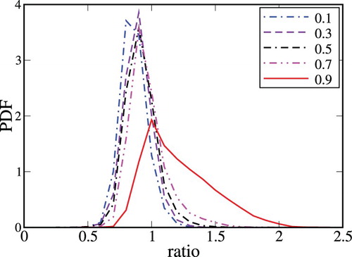
Figure 1 shows PDF $P_2\left(R_2,\overline{c}\right)$, see Equation (10), for a ratio of $R_2=\left(\mathrm{\nabla }\cdot \widehat{\rho D\mathrm{\nabla }c}+\hat{W}\right)/\left({\rho }_u{S}_L\widehat{|\mathrm{\nabla }c|}\right)$, obtained using $\mathrm{\Delta }/{\delta }_L=1.15$ at various values of the Reynolds-averaged combustion progress variable $\overline{c}$, specified in legends. The PDFs are sufficiently narrow and peak around unity, with the PDF width being reduced with increasing $\mathrm{\Delta }/{\delta }_L$ (not shown). A wider PDF obtained close to the trailing edge of the mean flame brush ($\overline{c}=0.9$, solid line) stems from significant perturbations of local flamelet structure in highly curved unburned mixture fingers, as discussed in details elsewhere [36,41]. All in all, Figure 1 well supports the FSD Equation (8), as could be expected for the studied conditions (flamelet combustion regime, single-step chemistry, and equidiffusive mixture).

Figure. 1. Probability Density Function $P_2\left(R_2,\overline{c}\right)$ for a ratio of $R_2=\left(\mathrm{\nabla }\cdot \widehat{\rho D\mathrm{\nabla }c}+\hat{W}\right)/\left({\rho }_u{S}_L\widehat{|\mathrm{\nabla }c|}\right)$, obtained using Equation (10) at $\mathrm{\Delta }/{\delta }_L=1.15$ and various values of the Reynolds-averaged combustion progress variable $\overline{c}$, specified in legends.

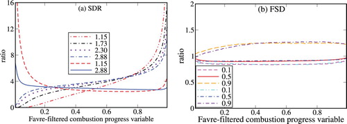
On the contrary, Figure 2(a) does not support apparently very similar SDR Equation (9) even under the present most favourable conditions, with qualitatively alike results being also obtained for $R_1$ and Equation (7). The PDFs $P_3\left(R_3,\overline{c}=0.5\right)$ are wide for all filters. At $\mathrm{\Delta }/{\delta }_L=2.30$ and 2.88, the PDFs peak between $R_3=2.5$ and 3.5, with the trend being more pronounced for the wider filter. The lower boundary of the peak interval is close to $2/\left(2c_m-1\right)=2.6$ calculated using the RANS value of $c_m=\overline{cW}/\overline{W}=0.88$ obtained by processing the same DNS data [27]. However, at lower $\mathrm{\Delta }/{\delta }_L=1.75$ and 1.73, such a peak is not observed and the PDFs monotonously decrease with $R_3$, but have high narrow peaks at $R_3\ll 1$. The latter peak is also observed, but less pronounced at $\mathrm{\Delta }/{\delta }_L=2.30$, see solid line. Such a peak could be attributed to chemically passive preheat zones characterised by sufficiently low local values of the combustion progress variable and vanishing rate $W\to 0$.

Figure 2. Probability Density Functions (a) $P_3\left(R_3,\overline{c}=0.5\right)$ and (b) $P_{\omega ,3}\left(\hat{\omega }=0.15\pm 0.005,R_3,\overline{c}=0.5\right)$ for a ratio of $R_3=\hat{W}/\widehat{\rho \chi }$. Different curves show results obtained using different normalised filter widths $\mathrm{\Delta }/{\delta }_L$, specified in legends.

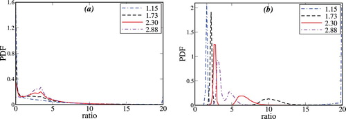
To exclude such an effect from consideration, Figure 2(b) shows joint PDF $P_{\omega ,3}\left(\hat{\omega }=0.15\pm 0.005,R_3,\overline{c}=0.5\right)$ obtained for a single $\hat{\omega }$-bin associated with sufficiently large filtered reaction rate. It is worth remembering that, due to a small thickness of a reaction zone characterised by $\omega \approx 1$, the maximal values of the filtered normalised rate $\hat{\omega }$ are as low as 0.52, 0.38, 0.34, and 0.31 for $\mathrm{\Delta }/{\delta }_L=1.15,$ 1.73, 2.30, and 2.88, respectively. The PDFs have well-pronounced bi-modal shape in all four cases (there is a large probability of $R_3\ge 20$ at $\mathrm{\Delta }/{\delta }_L=1.15$). While two peaks move to one another and tend to merge when the filter width is increased, the peaks are well separated even at the largest $\mathrm{\Delta }/{\delta }_L=2.88$ used here. Such a shape of the PDF is hardly consistent with Equation (9) and, therefore, puts it into question. Limitations of Equation (9) were earlier noted [15,45] by comparing dependencies of the conditioned $⟨\hat{W}\text{|}\widehat{\rho c}/\hat{\rho }⟩$ and $2⟨\widehat{\rho \chi }\text{|}\widehat{\rho c}/\hat{\rho }⟩/\left(2c_m-1\right)$ on $\widehat{\rho c}/\hat{\rho }$, extracted from DNS data using a Gaussian filter kernel of a small width $\mathrm{\Delta }$. However, the reported differences in $⟨\hat{W}\text{|}\widehat{\rho c}/\hat{\rho }⟩$ and $2⟨\widehat{\rho \chi }\text{|}\widehat{\rho c}/\hat{\rho }⟩/\left(2c_m-1\right)$ were claimed to be significantly reduced when increasing $\mathrm{\Delta }/{\delta }_L$ up to $3.02$ [15] and 2.8 [45], with $⟨D{a}_{\mathrm{\Delta }}\text{|}\widehat{\rho c}/\hat{\rho }⟩$ reaching 2.3 [15] and 4.5 [45]. The present analysis of the PDFs $P_3\left(R_3,\overline{c}\right)$ and $P_{\omega ,3}\left(\hat{\omega },R_3,\overline{c}\right)$ shows that Equation (9) performs poorly even if $\mathrm{\Delta }/{\delta }_L$ and $D{a}_{\mathrm{\Delta }}$ are as large as 2.88 and 60, respectively. It is also worth noting that even Figure 3 in Ref. [45], obtained using a filter with a large $\mathrm{\Delta }/\eta$, puts the LES SDR approach into question by indicating significant (more than 100%) differences in $⟨\hat{W}\text{|}\widehat{\rho c}/\hat{\rho }⟩$ and $2⟨\widehat{\rho \chi }\text{|}\widehat{\rho c}/\hat{\rho }⟩/\left(2c_m-1\right)$ at $⟨\widehat{\rho c}/\hat{\rho }⟩<0.2$ and $\mathrm{\Delta }/{\delta }_L=2.8$.

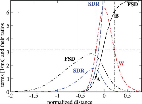
To explain results reported in Figure 2, let us consider the structure of the corresponding laminar flame. Figure 3 shows that the profiles of $\mathrm{\nabla }c\left(x\right)$, see double-dotted-dashed line, and $\rho \chi \left(x\right)$, see dotted-dashed line, are significantly shifted to the unburned side of the flame, when compared to the profile of $W\left(x\right)$, see double-dashed-dotted line. As a result, at sufficiently small $c$, i.e. at the normalised distance $\xi =x\text{max}\left\{|\mathrm{\nabla }c|\left(x\right)\right\}<-0.5$, the FSD $\mathrm{\nabla }c$ and SDR $\rho \chi$ can still have notable values, whereas the rate $W$ vanishes. Consequently, $W/\left({\rho }_u{S}_L\mathrm{\nabla }c\right)\to 0$, see short-dashed line, and $W/\left(\rho D\mathrm{\nabla }c\cdot \mathrm{\nabla }c\right)\to 0$, see long-dashed line, in such regions, which are, therefore, responsible for the PDF peak at $R_3\ll 1$ in Figure 2(a). On the contrary, in the vicinity of the peak $W\left(x\right)$ and, especially, at large $c$, i.e. at the normalised distance $\xi >0.25$, the ratios of $W/\left({\rho }_u{S}_L\mathrm{\nabla }c\right)$ and $W/\left(\rho D\mathrm{\nabla }c\cdot \mathrm{\nabla }c\right)$ are large, see short and long-dashed lines, respectively. Accordingly, for the same value of the normalised rate $\omega <1$, e.g. see dots on a horizontal line in Figure 3, there are two very different ratios of $W/\left({\rho }_u{S}_L\mathrm{\nabla }c\right)$ or $W/\left(\rho D\mathrm{\nabla }c\cdot \mathrm{\nabla }c\right)$, e.g. see points A and B on two vertical lines. Such two regions are responsible for the two PDF peaks shown in Figure 2(b). If a filter volume contains (i) the reaction zone (this is almost necessary in order for $\hat{\omega }$ to attain a value of 0.15) and (ii) points like A, then, such events control the PDF peak at a lower $R_3$. If a filter volume contains the reaction zone and points like B, such events control the PDF peak at a higher $R_3$.

Figure 3. Reaction rate $W/{\rho }_u$ (red double-dashed-dotted line), FSD $S_L\mathrm{\nabla }c$ (black double-dotted-dashed line), SDR $\rho D\mathrm{\nabla }c\cdot \mathrm{\nabla }c/{\rho }_u$ (blue dotted-dashed line), and ratios of $W/\left({\rho }_u{S}_L\mathrm{\nabla }c\right)$ (black short-dashed line) and $W/\left(\rho D\mathrm{\nabla }c\cdot \mathrm{\nabla }c\right)$ (blue long-dashed line) vs. the normalised distance $\xi =x\text{max}\left\{|\mathrm{\nabla }c|\left(x\right)\right\}$ counted from the position of peak rate $W/{\rho }_u$ in the laminar flame that propagates from right to left.

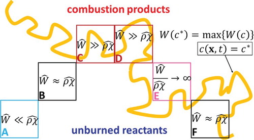
Such an interpretation of the obtained results is illustrated in Figure 4, where a curve shows an iso-surface of $\omega \left(\mathbf{\text{x}},t\right)=1$ or $c\left(\mathbf{\text{x}},t\right)=c^{\ast }$ and squares are associated with filter volumes. Square A is sufficiently far from the reaction zone, but contains the leading edge of the preheat zone. Accordingly, the rate $W$ almost vanishes in the entire square, whereas the SDR $\rho \chi$ may attain notable values at least in the part of the square. Consequently, square A is associated with $R_3\ll 1$. Squares B and F are sufficiently close to the curve $\omega \left(\mathbf{\text{x}},t\right)=1$ and even may contain it, but the largest parts of these squares contain mixture characterised by $c<c^{\ast }$. Accordingly, contributions from smaller regions associated with a high $W/\left(\rho D\mathrm{\nabla }c\cdot \mathrm{\nabla }c\right)$ may counterbalance contributions from lager regions associated with a low $W/\left(\rho D\mathrm{\nabla }c\cdot \mathrm{\nabla }c\right)$ so that the filtered values of $\hat{W}$ and $\widehat{\rho \chi }$ are close to one another. Squares C and D contain large pieces of the curve $\omega \left(\mathbf{\text{x}},t\right)=1$ and large regions characterised by $c>c^{\ast }$, whereas $c<c^{\ast }$ in smaller regions. Accordingly, see also Figure 3, squares C and D contribute to high $R_3$. Finally, $c\ge c^{\ast }$ in the largest part of square E, with this square being close to the curve $c\left(\mathbf{\text{x}},t\right)=c^{\ast }.$ Accordingly, the ratio of $W/\left(\rho D\mathrm{\nabla }c\cdot \mathrm{\nabla }c\right)$ integrated over square E may be very large, i.e. this square is associated with $R_3\gg 1$.

Figure 4. A 2D sketch of reaction zone (curve) and filter volumes.

To understand why the features discussed above make Equation (9) wrong (at least, locally), but do not affect Equation (8), let us consider the unperturbed laminar flame in the coordinate framework attached to it. For simplicity, the flame propagates from right to left. As already discussed in Introduction, in the flamelet combustion regime, flamelets retain the structure of the unperturbed laminar flame. Hence, locally, Equation (4) holds and, therefore, a ratio of $\left[\mathrm{\nabla }\cdot \left(\rho D\mathrm{\nabla }c\right)+W\right]/\left({\rho }_u{S}_L|\mathrm{\nabla }c|\right)$ is close to unity everywhere within flamelets, thus, resulting in $R_2\approx 1$ after filtering. Thus, Equation (8) works well under conditions of the present study, because Equation (8) is the local relation.

In the considered case of the laminar flame, multiplication of Equation (3) with $c$ results in (12) ${\rho }_u{S}_L\frac{\text{d}{c}^2}{\text{d}x}=2\frac{\text{d}}{\text{d}x}\left(\rho Dc\frac{\text{d}c}{\text{d}x}\right)-2\rho D{\left(\frac{\text{d}c}{\text{d}x}\right)}^2+2cW$(12) or (13) $\rho \chi =\frac{\text{d}}{\text{d}x}\left(\rho Dc\frac{\text{d}c}{\text{d}x}\right)-\frac{1}{2}{\rho }_u{S}_L\frac{\text{d}{c}^2}{\text{d}x}+cW.$(13)

Integration along the $x$-axis yields (14) ${\int }_{-\mathrm{\infty }}^{\mathrm{\infty }}\rho \chi \text{d}x=-\frac{1}{2}{\rho }_u{S}_L+{\int }_{-\mathrm{\infty }}^{\mathrm{\infty }}cW\text{d}x=-\frac{1}{2}{\int }_{-\mathrm{\infty }}^{\mathrm{\infty }}W\text{d}x+{\int }_{-\mathrm{\infty }}^{\mathrm{\infty }}cW\text{d}x,$(14) which look similar to Equation (2) or (9) if ${\int }_{-\mathrm{\infty }}^{\mathrm{\infty }}\rho \chi \text{d}x$, ${\int }_{-\mathrm{\infty }}^{\mathrm{\infty }}W\text{d}x$, and ${\int }_{-\mathrm{\infty }}^{\mathrm{\infty }}cW\text{d}x$ are associated with $\overline{\rho \chi }$ or $\widehat{\rho \chi }$, $\overline{W}$ or $\hat{W},$ and $c_m\overline{W}$ or $c_m\hat{W}$, respectively. Thus, the SDR approach is based on the integral features of flamelets, but the linear relation between $W$ and $\rho \chi$ does not hold locally in flamelets, see Equation (13), contrary to the local linear relation between $\mathrm{\nabla }\cdot \left(\rho D\mathrm{\nabla }c\right)+W$ and $|\mathrm{\nabla }c|$. Within the RANS framework, this difference between the FSD and SDR approaches is of minor importance, because averaging assumes integration over flamelets. Within the LES framework, the highlighted difference is of primary importance, because filtering is applied to a part of a flamelet, thus, making integral relations wrong.

Due to the effects discussed above, the ratio $⟨R_3\text{|}\widehat{\rho c}/\hat{\rho }⟩$ depends strongly on the filtered combustion progress variable $⟨\widehat{\rho c}/\hat{\rho }⟩$ that this ratio is conditioned to, see dotted and dotted-dashed lines in Figure 5(a) and note that close results were obtained at other $\overline{c}\left(x\right)$, with exception of the trailing edge of the flame brush (not shown). While the dependence of $⟨R_3\text{|}\widehat{\rho c}/\hat{\rho }⟩$. on $⟨\widehat{\rho c}/\hat{\rho }⟩$ is reduced with increasing filter width, it is well pronounced even for the largest filter $\mathrm{\Delta }/{\delta }_L=2.88$ (or $\mathrm{\Delta }/L_{11}=0.18$) used by us, see double-dashed-dotted line. Occasionally, substitution of $\hat{W}$ with $\mathrm{\nabla }\cdot \left(\widehat{\rho D\mathrm{\nabla }c}\right)+\hat{W}$ in Equation (9) yields substantially less pronounced dependence of the ratio $⟨R_4\text{|}\widehat{\rho c}/\hat{\rho }⟩=⟨\left(\mathrm{\nabla }\cdot \widehat{\rho D\mathrm{\nabla }c}+\hat{W}\right)/\widehat{\rho \chi }\text{|}\widehat{\rho c}/\hat{\rho }⟩$ on $⟨\widehat{\rho c}/\hat{\rho }⟩$ if the filter width is large, see solid line. However, such a substitution does not seem to have basic substantiation. In any case, even the dependence of $⟨R_4\text{|}\widehat{\rho c}/\hat{\rho }⟩$ on $⟨\widehat{\rho c}/\hat{\rho }⟩$ at the largest $\mathrm{\Delta }/{\delta }_L$ is much more pronounced than the dependence of $⟨R_2\text{|}\widehat{\rho c}/\hat{\rho }⟩$ on $⟨\widehat{\rho c}/\hat{\rho }⟩$ at low $\mathrm{\Delta }/{\delta }_L$, see Figure 5(b), thus, making the LES SDR approach inferior when compared to the LES FSD approach.

Figure 5. (a) Ratios $⟨R_3\text{|}\widehat{\rho c}/\hat{\rho }⟩=⟨\hat{W}/\widehat{\rho \chi }\text{|}\widehat{\rho c}/\hat{\rho }⟩$ (dotted-dashed and dotted lines) and $⟨R_4\text{|}\widehat{\rho c}/\hat{\rho }⟩=⟨\left(\mathrm{\nabla }\cdot \widehat{\rho D\mathrm{\nabla }c}+\hat{W}\right)/\widehat{\rho \chi }\text{|}\widehat{\rho c}/\hat{\rho }⟩$ (dashed and solid lines) conditioned to the filtered combustion progress variable $⟨\widehat{\rho c}/\hat{\rho }⟩$ and evaluated using various normalised filter widths $\mathrm{\Delta }/{\delta }_L$ specified in legends at the Reynolds-averaged combustion progress variable $\overline{c}=0.5$. (b) A ratio of $⟨R_2\text{|}\widehat{\rho c}/\hat{\rho }⟩=⟨\left(\mathrm{\nabla }\cdot \widehat{\rho D\mathrm{\nabla }c}+\hat{W}\right)/\left({\rho }_u{S}_L\hat{\mathrm{\Sigma }}\right)\text{|}\widehat{\rho c}/\hat{\rho }⟩$ conditioned to $⟨\widehat{\rho c}/\hat{\rho }⟩$ and evaluated using $\mathrm{\Delta }/{\delta }_L=1.15$ (solid and dashed lines) and 1.73 (dotted-dashed lines) at various values of the Reynolds-averaged combustion progress variable $\overline{c}$, specified in legends.

It is worth stressing that significant variations of the ratio $R_3$ within the turbulent flame brush strongly impede evaluating a ‘constant’ $c_m$ with the help of a method similar to Germano identity [3], which is widely used in LES research into turbulent flows. The identity is based on a hypothesis that application of two different filters to a model relation $\hat{Y}=bf\left(\widehat{\mathbf{\text{X}}}\right)$ yields the same value of the model constant $b$. Accordingly, the constant can be evaluated by comparing filtered fields $\hat{Y}$ and $\widehat{\mathbf{\text{X}}}$ with double-filtered fields $\widehat{\stackrel{ˆ}{Y}}$ and $\stackrel{ˆ}{\widehat{\mathbf{\text{X}}}}$. The method can yield correct results even if the values of $b$ computed in various cells are not constant, but are randomly scattered around a mean value [3]. However, the method may yield wrong results if $b$ correlates with $\widehat{\mathbf{\text{X}}}$ and/or $\hat{Y}$. In such a case, significant errors can be obtained even when analysing the same LES field.

For instance, because $W=\rho \chi \cdot \left(W/\rho \chi \right)$, one can assume that $\hat{W}=\widehat{\left(W/\rho \chi \right)\rho \chi }=\widehat{\left(W/\rho \chi \right)}\widehat{\rho \chi }=C_{\chi }\widehat{\rho \chi }$, where the model ‘constant’ $C_{\chi }$ is evaluated by properly averaging the ratio $R_3=\hat{W}/\widehat{\rho \chi }$ instead of invoking $C_{\chi }=2/\left(2c_m-1\right)$ in Equation (9). However, such a method yields wrong results even if LES fields are averaged and obtained RANS data are analysed. For instance, if $C_{\chi }$ is associated with volume or transverse averaged (in cells characterised by $0.01<\hat{c}\left(\mathbf{\text{x}},t\right)<0.99$) LES fields $R_3=\hat{W}/\widehat{\rho \chi }$, then, such a model substantially overestimates the mean rate $\overline{\hat{W}}/{\rho }_u$, cf. curves 3 and 4, respectively, with curve 1 in Figure 6. The point is that terms $\rho \chi$ and $\left(W/\rho \chi \right)$ in $\widehat{\rho \chi \left(W/\rho \chi \right)}$ correlate negatively (the ratio of $W/\rho \chi$ is large when the scalar dissipation is low, see range $\xi >0$ in Figure 3, and vice versa) and, if this negative correlation is disregarded by assuming that $\widehat{\rho \chi \left(W/\rho \chi \right)}=C_{\chi }\widehat{\rho \chi }$, then, the mean reaction rate is overestimated. This example shows that ideas by Germano et al. [3] should not be applied to a quantity which is considered to be a constant within the RANS framework, but may significantly vary in LES.

Figure 6. Mean reaction rate vs. Reynolds-averaged combustion progress variable $\overline{c}$. 1 – $\overline{\hat{W}}/{\rho }_u$. 2 – $2\overline{\widehat{\rho \chi }}/\left[{\rho }_u\left(2c_m-1\right)\right]$, where $c_m=0.88$ [27], 3 – $⟨R_3⟩\overline{\widehat{\rho \chi }}/{\rho }_u$, where the ratio $⟨R_3⟩=⟨\hat{W}/\widehat{\rho \chi }⟩$ is averaged over all cells characterised by $0.01<\hat{c}\left(\mathbf{\text{x}},t\right)<0.99$, 4 – $\overline{R_3}\overline{\widehat{\rho \chi }}/{\rho }_u$, where the ratio $\overline{R_3}\left(\overline{c}\right)$ is averaged over transverse plane provided that $0.01<\hat{c}\left(\mathbf{\text{x}},t\right)<0.99$. $\mathrm{\Delta }/{\delta }_L=2.88$.

On the contrary, curves 1 and 2 in Figure 6 show that Equation (9) with $c_m=0.88$ taken from RANS simulations [27] well predicts the mean (Reynolds-averaged) profile of $\overline{\hat{W}}\left(\overline{c}\right)/{\rho }_u$ in spite of the fact that the LES Equation (9) is not supported by the present DNS data for filtered quantities. This result is not surprising. Indeed, if filtering and taking a mean commute, i.e. $\overline{\hat{q}}=\hat{\overline{q}}$ for any quantity $q\left(\mathbf{\text{x}},t\right)$, and a model relation $\overline{Y}=b\overline{X}$ holds within the RANS framework, then, even if $\hat{Y}\ne b\hat{X}$, nevertheless, $\overline{\hat{Y}}=b\overline{\hat{X}}=b\hat{\overline{X}}=\hat{\overline{Y}}\approx \overline{Y}$ provided that the filter width is sufficiently small. However, if LES output is solely reduced to mean quantities, then, it seems to be equivalent to filtered RANS results and, therefore, such a limited LES study does not appear to be superior with respect to the RANS simulation. The use of a more expensive LES approach instead of RANS computation should be warranted by extra data obtained in the LES. This is necessary, but is not sufficient. Indeed, the LES results should not only provide more information, but the extra data should be valid. Therefore, a thorough test of a LES combustion model should not be reduced to comparing averaged computed fields with experimental or DNS data, but should also validate filtered fields. Otherwise, good test results obtained for the averaged data, e.g. curve 2 in Figure 6, can lead to a wrong conclusion regarding validity of the LES closure relation, e.g. Equation (9), which is put into question by results plotted in Figures 2 and 5(a).

There is another relevant issue also. Since the poor performance of Equation (9) results from the non-local nature of this relation, one could assume that Equation (9) is sufficiently precise (in the flamelet combustion regime) provided that the filter width is appropriately large. Indeed, if a filter volume is much larger than ${\delta }_L$, then, the flamelet elements that are partly outside the volume contribute to the filtered $\hat{W}$ and $\widehat{\rho \chi }$ much less than the flamelet elements that are entirely in the volume, and Equation (9) should hold due to integration over the latter flamelet elements (in the flamelet combustion regime). However, an increase in a filter width has also negative consequences. The point is that filtering not only smooths out small-scale fluctuations, e.g. due to integration over transverse plane in the statistically planar 1D case, but also smooths spatial variations in the direction normal to the mean flame brush, e.g. in the $x$-direction in that case. Accordingly, an increase in a filter width can impede comparing LES and experimental data if the width is too large. In the aforementioned 1D case, the problem can be circumvented by using a 2D filter, i.e. by integrating instantaneous fields over a square at a constant $x$, but such a method is difficult to be applied in a general case. While results plotted in Figures 2 and 5(a) show that an increase in $\mathrm{\Delta }/{\delta }_L$ is beneficial for the LES-SDR approach, the effect is quite moderate and results obtained at $\mathrm{\Delta }/{\delta }_L=2.88$ are still poor. Accordingly, Equation (9) does not seem to be valid for filter widths that are sufficiently small to permit direct comparison of LES results with experimental data.

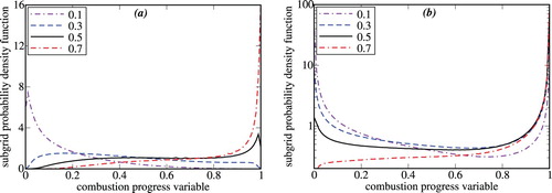
Finally, Figure 7 shows that the probability of finding intermediate values of $c$ is substantial for the range of $\mathrm{\Delta }/{\delta }_L$ investigated in the present work, i.e. subgrid conditioned PDFs $\hat{P}\left(c|\hat{c}\right)$ are not exactly bimodal, while the shape of $\hat{P}\left(c|\hat{c}\right)$ tends to the bimodal one when $\mathrm{\Delta }/{\delta }_L$ is increased, cf. Figure 7(a,b) and note the subgrid PDFs are shown in linear and logarithmic, respectively, scales in the two subfigures. Accordingly, a modified LES-SDR approach could be developed invoking a non-bimodal $\hat{P}\left(c\right)$. Such PDFs were recently introduced [46,47] by extending the classical BML approach [6]. However, this task is beyond the scope of the present work.

Figure 7. Subgrid conditioned PDFs $\hat{P}\left(c|\hat{c}\right)$ obtained at $\overline{c}=0.5$ and (a) $\mathrm{\Delta }/{\delta }_L=1.15$ or (b) $\mathrm{\Delta }/{\delta }_L=2.88$. Note that the PDFs are shown in linear and logarithmic scales in (a) and (b), respectively. The PDF sampling was performed for all grid points within a filter volume centred around a point $\mathbf{\text{x}}$ at instant $t$, followed by averaging the PDFs $P\left(c,\mathbf{\text{x}},t\right)$ for all $\mathbf{\text{x}}$ and $t$ such that ${\hat{c}}^{\ast }+0.005\le \hat{c}\left(\mathbf{\text{x}},t\right)<{\hat{c}}^{\ast }+0.005$. Values of ${\hat{c}}^{\ast }$ are specified in legends.

It is also worth remembering that the LES counterpart of another cornerstone assumption by Bray [6,7], i.e. length scales characterising spatial variations of $c$ and $\mathrm{\nabla }c$ are much less than length scales characterising spatial variations of the filtered values of these quantities, is unlikely to hold if the filter width and the laminar flame thickness are of the same order. If the filter width is significantly increased, the fundamental limitations of the LES SDR approach emphasised in the present paper may be mitigated. However, as already discussed in Sect. 2, such a significant increase in $\mathrm{\Delta }$ will make the LES SDR approach inferior to RANS SDR approach under conditions the approach was originally developed for [5,6,10], i.e. in the flamelet combustion regime associated with a large ratio of $\eta /{\delta }_L$.

4. Conclusions

Linear Relations between (i) filtered reaction rate and filtered flame surface density and (ii) filtered reaction rate and filtered scalar dissipation rate, which are widely used in LES research into premixed turbulent combustion, were examined by processing DNS data obtained under weakly turbulent conditions that are most favourable for the two approaches (flamelet combustion regime, single-step chemistry, equidiffusive mixture, adiabatic burner, and low Mach number). The analysis well supports the former approach provided that the filtered reaction rate is combined with filtered molecular transport term. In such a case, both the RANS and LES FSD approaches are based on local relations valid within weakly perturbed flamelets. Therefore, simply recasting RANS expressions to a filtered form works well. On the contrary, while the FSD and SDR approaches appear to be basically similar at first glance, the analysis does not support the latter one, but shows that a ratio of the filtered reaction rate to the filtered SDR is strongly scattered within the studied flame brush, with its conditionally mean value varying significantly with Favre-filtered combustion progress variable. The point is that the SDR approach is based on a relation that holds after integration over weakly perturbed flamelets, but does not hold locally within such flamelets. Consequently, when a sufficiently small filter is applied to instantaneous fields, the filter may contain only a part of the local flamelet volume, whereas the linear relation holds solely for the entire flamelet and may not hold within the filtered flamelet volume. Thus, the present study indicates that straightforwardly recasting well-established RANS equations to a filtered form may be a flawed approach to modelling subgrid flame-turbulence interaction if the equations are based on integral features of local burning.

Disclosure statement

No potential conflict of interest was reported by the authors.

Additional information

Funding

The first author gratefully acknowledges financial support by Chalmers Area of Advance Transport and Combustion Engine Research Center (CERC).

References

- L.Y.M. Gicquel, G. Staffelbach, and T. Poinsot, Large Eddy simulations of gaseous flames in gas turbine combustion chambers, Prog. Energy Combust. Sci. 38 (2012), pp. 782–815. doi: 10.1016/j.pecs.2012.04.004
- T. Poinsot, Prediction and control of combustion instabilities in real engines, Proc. Combust. Inst. 36 (2017), pp. 1–28. doi: 10.1016/j.proci.2016.05.007
- M. Germano, U. Piomelli, P. Moin, and W.H. Cabot, A dynamic subgrid-scale eddy viscosity model, Phys Fluids A. 3 (1991), pp. 1760–1765. doi: 10.1063/1.857955
- D. Veynante and L. Vervisch, Turbulent combustion modeling, Prog. Energy Combust. Sci. 28 (2002), pp. 193–266. doi: 10.1016/S0360-1285(01)00017-X
- N. Chakraborty, M. Champion, A. Mura, and N. Swaminathan, Scalar-dissipation-rate approach, in Chapter 4 of Turbulent premixed flames, N. Swaminathan and K.N.C. Bray, eds., Cambridge University Press, Cambridge, 2011, pp. 76–102.
- K.N.C. Bray, Turbulent flows with premixed reactants, in Chapter 4 of Turbulent reacting flows, P.A. Libby and F.A. Williams, eds., Springer-Verlag, Berlin, 1980, pp. 115–183.
- K.N.C. Bray, The interaction between turbulence and combustion, Proc. Combust. Inst. 17 (1979), pp. 223–233. doi: 10.1016/S0082-0784(79)80024-7
- P. Clavin, Dynamical behavior of premixed flame fronts in laminar and turbulent flows, Prog. Energy Combust. Sci. 11 (1985), pp. 1–59. doi: 10.1016/0360-1285(85)90012-7
- M. Matalon, Flame dynamics, Proc. Combust. Inst. 32 (2009), pp. 57–82. doi: 10.1016/j.proci.2008.08.002
- R. Borghi, Turbulent premixed combustion: further discussions of the scales of fluctuations, Combust Flame. 80 (1990), pp. 304–312. doi: 10.1016/0010-2180(90)90106-2
- M. Boger, D. Veynante, H. Boughanem, and A. Trouvé, Direct numerical simulation analysis of flame surface density concept for large-eddy simulation of turbulent premixed combustion, Proc. Combust. Inst. 27 (1998), pp. 917–925. doi: 10.1016/S0082-0784(98)80489-X
- E.R. Hawkes and R.S. Cant, A flame surface density approach to Large-Eddy simulation of premixed turbulent combustion, Proc. Combust. Inst. 28 (2000), pp. 51–58. doi: 10.1016/S0082-0784(00)80194-0
- T. Ma, O.T. Stein, N. Chakraborty, and A.M. Kempf, A posteriori testing of the flame surface density transport equation for LES, Combust. Theory Model. 18 (2014), pp. 32–64. doi: 10.1080/13647830.2013.848383
- C.Y. Lee and S. Cant, Large-eddy simulation of a bluff-body stabilised turbulent premixed flame using the transported flame surface density approach, Combust. Theory Model. 21 (2017), pp. 722–748. doi: 10.1080/13647830.2017.1293849
- T.D. Dunstan, Y. Minamoto, N. Chakraborty, and N. Swaminathan, Scalar dissipation rate modelling for Large Eddy simulation of turbulent premixed flames, Proc. Combust. Inst. 34 (2013), pp. 1193–1201. doi: 10.1016/j.proci.2012.06.143
- I. Langella, N. Swaminathan, Y. Gao, and N. Chakraborty, Assessment of dynamic closure for premixed combustion Large Eddy simulation, Combust. Theory Model. 19 (2015), pp. 628–656. doi: 10.1080/13647830.2015.1080387
- Y. Gao and N. Chakraborty, Modeling of Lewis number dependence of scalar dissipation rate transport for Large Eddy simulations of turbulent premixed combustion, Num. Heat Transfer A: Applications. 69 (2016), pp. 1201–1222. doi: 10.1080/10407782.2015.1125732
- M.J. Cernick, S.W. Tullis, and M.F. Lightstone, Particle subgrid scale modelling in Large-Eddy simulations of particle-laden turbulence, J. Turbul. 16 (2015), pp. 101–135. doi: 10.1080/14685248.2014.969888
- D.H. Rowinski and S.B. Pope, Computational study of lean premixed turbulent flames using RANS PDF and LES PDF methods, Combust. Theory Model. 17 (2013), pp. 610–656. doi: 10.1080/13647830.2013.789929
- S. Nishiki, T. Hasegawa, R. Borghi, and R. Himeno, Modelling of flame-generated turbulence based on direct numerical simulation databases, Proc. Combust. Inst. 29 (2002), pp. 2017–2022. doi: 10.1016/S1540-7489(02)80246-2
- S. Nishiki, T. Hasegawa, R. Borghi, and R. Himeno, Modelling of turbulent scalar flux in turbulent premixed flames based on DNS databases, Combust. Theory Modelling. 10 (2006), pp. 39–55.
- H.A. Uranakara, S. Chaudhuri, H.L. Dave, P.G. Arias, and H.G. Im, A flame particle tracking analysis of turbulence-chemistry interaction in hydrogen-air premixed flames, Combust Flame. 163 (2016), pp. 220–240. doi: 10.1016/j.combustflame.2015.09.033
- A.J. Aspden, M.J. Day, and J.B. Bell, Three-dimensional direct numerical simulation of turbulent lean premixed methane combustion with detailed kinetics, Combust Flame. 166 (2016), pp. 266–283. doi: 10.1016/j.combustflame.2016.01.027
- S. Lapointe and G. Blanquart, Fuel and chemistry effects in high Karlovitz premixed turbulent flames, Combust Flame. 167 (2016), pp. 294–307. doi: 10.1016/j.combustflame.2016.01.035
- H. Wang, E.R. Hawkes, B. Zhou, J.H. Chen, Z. Li, and M. Aldén, A comparison between direct numerical simulation and experiment of the turbulent burning velocity-related statistics in a turbulent methane-air premixed jet flame at high Karlovitz number, Proc. Combust. Inst. 36 (2017), pp. 2045–2053. doi: 10.1016/j.proci.2016.07.104
- S. Chaudhuri, H. Kolla, H.L. Dave, E.R. Hawkes, J.H. Chen, and C.K. Law, Flame thickness and conditional scalar dissipation rate in a premixed temporal turbulent reacting jet, Combust Flame. 184 (2017), pp. 273–285. doi: 10.1016/j.combustflame.2017.02.027
- A.N. Lipatnikov, S. Nishiki, and T. Hasegawa, DNS assessment of relation between mean reaction and scalar dissipation rates in the flamelet regime of premixed turbulent combustion, Combust. Theory Modell. 19 (2015), pp. 309–328. doi: 10.1080/13647830.2015.1021837
- A.N. Lipatnikov, V.A. Sabelnikov, S. Nishiki, and T. Hasegawa, Flamelet perturbations and flame surface density transport in weakly turbulent premixed combustion, Combust. Theory Modell. 21 (2017), pp. 205–227. doi: 10.1080/13647830.2016.1214750
- Y.H. Im, K.Y. Huh, S. Nishiki, and T. Hasegawa, Zone conditional assessment of flame-generated turbulence with DNS database of a turbulent premixed flame, Combust Flame. 137 (2004), pp. 478–488. doi: 10.1016/j.combustflame.2004.03.006
- A. Mura, K. Tsuboi, and T. Hasegawa, Modelling of the correlation between velocity and reactive scalar gradients in turbulent premixed flames based on DNS data, Combust. Theory Modelling. 12 (2008), pp. 671–698. doi: 10.1080/13647830801975154
- A. Mura, V. Robin, M. Champion, and T. Hasegawa, Small scale features of velocity and scalar fields in turbulent premixed flames, Flow Turbul. Combust. 82 (2009), pp. 339–358. doi: 10.1007/s10494-008-9180-0
- V. Robin, A. Mura, M. Champion, and T. Hasegawa, Modelling of the effects of thermal expansion on scalar turbulent fluxes in turbulent premixed flames, Combust. Sci. Technol. 182 (2010), pp. 449–464. doi: 10.1080/00102200903462896
- V. Robin, A. Mura, and M. Champion, Direct and indirect thermal expansion effects in turbulent premixed flames, J. Fluid Mech. 689 (2011), pp. 149–182. doi: 10.1017/jfm.2011.409
- K.N.C. Bray, M. Champion, P.A. Libby, and N. Swaminathan, Scalar dissipation and mean reaction rates in premixed turbulent combustion, Combust Flame. 158 (2011), pp. 2017–2022. doi: 10.1016/j.combustflame.2011.03.009
- A.N. Lipatnikov, S. Nishiki, T. Hasegawa, A direct numerical simulation study of vorticity transformation in weakly turbulent premixed flames, Phys Fluids. 26 (2014), pp. 105104-1–105104-16. doi: 10.1063/1.4898640
- A.N. Lipatnikov, J. Chomiak, V.A. Sabelnikov, S. Nishiki, and T. Hasegawa, Unburned mixture fingers in premixed turbulent flames, Proc. Combust. Inst. 35 (2015), pp. 1401–1408. doi: 10.1016/j.proci.2014.06.081
- A.N. Lipatnikov, V.A. Sabelnikov, S. Nishiki, T. Hasegawa, and N. Chakraborty, DNS assessment of a simple model for evaluating velocity conditioned to unburned gas in premixed turbulent flames, Flow Turbul. Combust. 94 (2015), pp. 513–526. doi: 10.1007/s10494-014-9588-7
- V.A. Sabelnikov, A.N. Lipatnikov, N. Chakraborty, S. Nishiki, and T. Hasegawa, A transport equation for reaction rate in turbulent flows, Phys Fluids. 28 (2016), pp. 081701-1–081701-7. doi: 10.1063/1.4960390
- V.A. Sabelnikov, A.N. Lipatnikov, N. Chakraborty, S. Nishiki, and T. Hasegawa, A balance equation for the mean rate of product creation in premixed turbulent flames, Proc. Combust. Inst. 36 (2017), pp. 1893–1901. doi: 10.1016/j.proci.2016.08.018
- A.N. Lipatnikov, V.A. Sabelnikov, N. Chakraborty, S. Nishiki, and T. Hasegawa, A DNS study of closure relations for convection flux term in transport equation for mean reaction rate in turbulent flow, Flow Turbul. Combust. 100 (2018), pp. 75–92. doi: 10.1007/s10494-017-9833-y
- A.N. Lipatnikov, J. Chomiak, V.A. Sabelnikov, S. Nishiki, and T. Hasegawa, A DNS study of the physical mechanisms associated with density ratio influence on turbulent burning velocity in premixed flames, Combust. Theory Modell. 22 (2018), pp. 131–155. doi: 10.1080/13647830.2017.1390265
- A.N. Lipatnikov, V.A. Sabelnikov, S. Nishiki, T. Hasegawa, Combustion-induced local shear layers within premixed flamelets in weakly turbulent flows, Phys Fluids. 30 (2018), pp. 085101-1–085101-10.
- A.N. Lipatnikov, V.A. Sabelnikov, S. Nishiki, T. Hasegawa, Does flame-generated vorticity increase turbulent burning velocity?, Phys Fluids. 30 (2018), pp. 081702-1–081702-3.
- V.A. Sabelnikov, A.N. Lipatnikov, S. Nishiki, and T. Hasegawa, Application of conditioned structure functions to exploring influence of premixed combustion on two-point turbulence statistics, Proc. Combust. Inst. 37, in press.
- Y. Gao, N. Chakraborty, and N. Swaminathan, Algebraic closure of scalar dissipation rate for Large Eddy simulations of turbulent premixed combustion, Combust. Sci. Technol. 186 (2014), pp. 1309–1337. doi: 10.1080/00102202.2014.934581
- M.M. Salehi and W.K. Bushe, Presumed PDF modeling for RANS simulation of turbulent premixed flames, Combust. Theory Modell. 14 (2010), pp. 381–403. doi: 10.1080/13647830.2010.489957
- K.Q.N. Kha, V. Robin, A. Mura, and M. Champion, Implications of laminar flame finite thickness on the structure of turbulent premixed flames, J. Fluid Mech. 787 (2016), pp. 116–147. doi: 10.1017/jfm.2015.660