Lambert W function for effect of gas compression on premixed flames with ignition temperature approximation

Abstract

The assumption that the gradient of temperature at the burned-side edge of a premixed flame front is zero has been usually imposed in investigating the adiabatic profile of flames for quasi-isobaric flow or in the zero-Mach-number limit. However, the non-monotonic behaviour of temperature is also observed for flames, or deflagrations, in the process of deflagration-to-detonation transition inside tubes or in the context of laser ablation or thermonuclear explosions in the universe. This non-adiabatic profile of a flame front is mainly due to the effect of gas compression, which is different from the conductive or volumetric heat loss. To clarify this point, we derive the non-zero condition of temperature gradient by considering the additional region, or the compression zone, behind a freely propagating flame front. The method of singular perturbations, or matched asymptotic expansions, is employed to calculate the inner and outer solutions of the compression zone of $O\left({Ma}^2\right)$ thickness with the squared Mach number assumed to be small, ${Ma}^2\ll 1$. The inner solutions are expressed by use of Lambert W function, and the pressure and dissipation terms in the heat-conduction equation play an important role to capture the non-adiabaticity of a flame front for non-zero values of Mach number. The strong ignition temperature approximation is imposed to obtain exact solutions in the outer region, composed of the reaction and preheat zones. The adiabatic value of ignition temperature is determined. The non-adiabatic feature is categorised into two cases. One case shows the non-monotonic behaviour of temperature. The other case presents the monotonic profile of temperature, but its maximum value is beyond the adiabatic value. The boundary, which determines whether the compressibility effect increases or decreases the flame temperature, is given with respect to the values of ignition temperature, heat release and Prandtl number.

Keywords:

• non-adiabatic premixed flame
• compressibility
• ignition temperature
• singular perturbations
• Lambert W function

1. Introduction

In the thermal theory of a premixed flame front, where the quasi-isobaric flow is considered in the zero-Mach-number limit, its adiabatic profile is characterised by the monotonic increase of temperature in approaching the front from the unburned side [1,2]. The temperature takes its maximum value behind a flame front and keeps it constant in the entire region on the burned side. The temperature gradient is often assumed to be zero at the exit of a flame front on the burned side [3]. In the situation of one-dimensional flow, where a thin planar flame front is located at z = 0 and propagates in the negative z-direction, the assumption is given, with T temperature, by (1) $\frac{\mathrm{d}T}{\mathrm{d}z}{|}_{z=0+}=0.$(1) This assumption helps the analysis of inner structure of a flame front, the reaction zone. The large activation energy asymptotics is the powerful method to obtain the boundary conditions across the reaction zone [4,5] and to calculate the laminar flame speed or the burning-rate eigenvalue [6–8]. Such boundary conditions are in turn used to investigate the cellular or oscillatory instability [9] and to study the preheat zone structure or the hydrodynamic instability [10–14]. Inside the reaction zone, the solution of temperature is assumed to be in power series with respect to the inverse of large parameter β, the Zel'dovich number [15–17]. The temperature is assumed to be constant at the leading order, $O\left({\text{β}}^0\right)$. Then, the heat-conduction equation needs to be solved numerically to know the behaviour of solution at $O\left({\text{β}}^{-1}\right)$ [18].

The non-adiabatic feature of a flame front for quasi-isobaric flow has also been studied by use of the large activation energy asymptotics: for example, non-adiabatic temperature profile of a diffusion flame [19] and the quenching due to the volumetric heat loss of a premixed flame [20,21] and the conductive heat loss [22]. For the case of volumetric heat loss, the non-adiabatic feature of a flame front was realised by introducing the sink term into the heat-conduction equation. The sink term usually has the expression of Newton's law of cooling [23] or thermal radiation type [24]. The analysis of non-adiabatic flames without (1(1) $\frac{\mathrm{d}T}{\mathrm{d}z}{|}_{z=0+}=0.$(1) ) has been performed, for example, by [25]. In [25], the non-constant behaviour of temperature on the burned side of a flame front was well captured by considering the additional zone or the convective-loss zone. However, the above works restricted themselves to the incompressible case: the effect of pressure and dissipation terms in the heat-conduction equation was neglected due to zero-Mach-number limit. These effect should be accounted for in considering the effect of compressibility or finite Mach number.

The importance of gas compressibility appears with practical interest in the wide variety of combustion phenomena: for example, inside tubes [26,27], in the context of laser ablation [28,29] or in the process of thermonuclear explosions in the universe [30,31]. Inside tubes, the effects of wall friction and thermal expansion are important to understand the acceleration of a flame front [32,33]. Besides, the effect of pressure due to the closed ends of channel enhances the flame temperature [34]. The rise of burning rate largely depends on the Darrieus–Landau instability (DLI) which is an intrinsic instability of flames induced by thermal expansion [35,36]. It has been shown that the flame acceleration is weaken by gas compression theoretically through small Mach number expansions up to first order terms [37,38]. However, the mechanism of deflagration-to-detonation transition (DDT) remains unclear and its resolution is demanded in practice: for example, the safety strategies against a mining accident in a gaseous-dusty coal mining environment [39] or the comprehension of local expansion rate of the universe [30].

In studying the DDT, the deflagration and the detonation are sometimes considered separately due to its complexity. The analysis of deflagrations, or flames, is actively performed in the context of the Type Ia supernova (SN Ia) which is the thermonuclear explosion observed in degenerate stars or white dwarfs [40,41]. If the initial overpressure due to the heat of burning products is too weak, the classical thermal theory of a flame front consisting of preheat and reaction zones is applicable for the study of SN Ia, for example, by considering the burning of premixed carbon-oxygen fuel [42,43]. In the pure deflagration model for the SN Ia, the laminar flame speed needs to be considered in the range of ${10}^4-{10}^7$ cm s${}^{-1}$ [30]. Correspondingly, the Mach number takes its value in the range of 0.01−0.1 [44–46]. The numerical simulation for flames propagating with small Mach numbers in the SN Ia shows that the temperature takes its maximum value inside the reaction front and decreases on the burned side [47].

The consideration of small Mach numbers may be meaningful also in the study of detonation. The pioneering work of steady one-dimensional detonation was performed by Zel'dovich [48], von Neumann [49] and Döring [50] and their result is called ZND theory. In the framework of ZND theory, the detonation is considered to be composed of the leading shock front and the succeeding reaction front. Focusing on the temperature profile, ZND theory indicates the non-monotonic behaviour of temperature with its maximum value reached inside the reaction zone. The same tendency of temperature is also obtained for the SN Ia in the context of detonation model [51,52] and reconstruction model [53]. Although the velocity of incoming flow ahead of the shock is supersonic, the flow field behind the shock is subsonic. Especially, the physical quantities evaluated immediately behind the shock are called Neumann state. The representative values of Mach number for Neumann state are approximately around 0.2 [54]. These values may correspond to those treated in our study, which are evaluated locally in the far-field from the front on the unburned side. In this sense, our model may be adoptable to the estimation of flow properties behind the shock by associating the far-field boundary conditions with the Neumann state. In fact, the deflagration and detonation modes are treated separately in [53]. Although the multidimensional structure of detonation front should be taken into account for practical interest in the DDT scenario [42], the treatment of two- or three-dimensional flow fields is devoted to future work.

In this study, we assume that the squared Mach number is sufficiently small, ${Ma}^2\ll 1$ and consider the compression zone of $O\left({Ma}^2\right)$ thickness behind a flame front to reveal the effect of gas compressibility. The introduction of additional region has also been employed in the previous works [55,56]. Our model may be adopted to study the thermonuclear flame front by considering that it consists of three regions: preheat, reaction and compression zones. Indeed, the peak structure of temperature inside the reaction zone is well captured by use of asymptotic solutions. This result may be compared qualitatively with that obtained numerically in previous works [47,51–53]. In addition, the temperature gradient at the interface between the reaction and compression zones is derived and explicitly given by the deviation of thermal expansion rate from its adiabatic value. Although the DLI is a primary concern for the formation of corrugated front, which results in the acceleration of flame propagation speed in the DDT, we restrict ourselves to the study of a steady one-dimensional flame front. However, our analysis is performed in the small scale of thermal thickness of a flame front and may be used as the local estimation for fast flames. As for the SN Ia, the Rayleigh-Taylor instability due to buoyancy effect is essential for the formation of turbulence [31]. The effect of curvature or gravitational acceleration on flames will be treated in the future work.

Instead of (1(1) $\frac{\mathrm{d}T}{\mathrm{d}z}{|}_{z=0+}=0.$(1) ), we derive the non-zero condition of temperature gradient for a non-adiabatic flame front by studying the compression zone based on the method of matched asymptotic expansions [57]. The inner and outer solutions are assumed to be in power series with respect to ${Ma}^2(\ll 1)$ and calculated up to $O\left({Ma}^2\right)$ terms in order to know the effect of compressibility. Inside the compression zone, the governing equations are solved analytically and inner solutions are found to be expressed by use of Lambert W function, which is defined as the inverse relation of $z{\mathrm{e}}^z$ [58]. Through the calculation of inner solutions, we find that the non-adiabatic feature is induced by the pressure and dissipation terms in the heat-conduction equation. Therefore, unlike the conductive or volumetric heat loss, we obtain the temperature decrease due to the gas compression for small but non-zero values of Mach number.

We use the length scale of preheat zone as the characteristic one in order to non-dimensionalise the governing equations. Therefore, the $O\left(1\right)$ region outside the compression zone implies the internal structure of a flame front, composed of the preheat and reaction zones. Instead of the large activation energy asymptotics, we employ the strong ignition temperature approximation [59–62]. This is because it becomes possible to obtain exact solutions in the outer region on the unburned side by assuming that the reaction rate is constant inside the reaction zone and zero outside it. In this case, the upstream edge of the reaction zone is identified by introducing the concept of ignition temperature. The position dividing the preheat and reaction zones is found to be given by the inverse of reaction rate. Then, both of the increase of temperature and the decrease of width of reaction zone are simultaneously brought about by the rise of reaction rate [21,63]. Outer solutions are connected with inner ones to give the smooth adiabatic or non-adiabatic profile of temperature depending on the values of ignition temperature. Especially, the value of adiabatic ignition temperature is determined.

The non-adiabatic feature due to gas compression is categorised into two cases. One case shows the non-monotonic behaviour of temperature. The other case presents the monotonic profile of temperature but its maximum value is beyond the adiabatic value. The boundary, which determines whether the compressibility effect increases or decreases the flame temperature, is given with respect to the values of ignition temperature, heat release and Prandtl number. Although the strong ignition temperature approximation brings the demerit of cold boundary difficulty, the resolution of this difficulty will be treated in the future work by considering the temperature dependence of reaction rate, for example, according to [64,65].

The paper is organised as follows. In Section 2, governing equations are presented and we recall the matching conditions between inner and outer solutions in the overlapping region. The analysis of the inner region, or the compression zone, is performed in Section 3. Then, the outer regions are studied in Section 4. Our main results are in Section 5 and the conclusions follow in Section 6.

2. Preliminaries

2.1. Governing equations

We consider a planar premixed flame front propagating in the negative z-direction. The coordinate z is non-dimensionalised by the thermal thickness of a flame front or the length scale of preheat zone [3]. For simplicity, the flow field is assumed to be one-dimensional. This assumption is not essential because the analysis of compression zone reduces to that of one-dimensional flow even when we consider two- or three-dimensional flow. The following governing equations are non-dimensionalised by quantities in the far field from a flame front on the unburned side, $z\to -\mathrm{\infty }$. (2) $\begin{array}{rl}\frac{\mathrm{d}M}{\mathrm{d}z}& =0,\end{array}$(2) (3) $\begin{array}{rl}M\frac{\mathrm{d}V}{\mathrm{d}z}& =-\frac{1}{\gamma {Ma}^2}\frac{\mathrm{d}P}{\mathrm{d}z}+\frac{4}{3}Pr\frac{{\mathrm{d}}^{2}V}{\mathrm{d}{z}^2},\end{array}$(3) (4) $\begin{array}{rl}M\frac{\mathrm{d}T}{\mathrm{d}z}& =\frac{{\mathrm{d}}^{2}T}{\mathrm{d}{z}^2}+\frac{\gamma -1}{\gamma }V\frac{\mathrm{d}P}{\mathrm{d}z}+\frac{4}{3}(\gamma -1)Pr{Ma}^2{\left(\frac{\mathrm{d}V}{\mathrm{d}z}\right)}^2+qQ,\end{array}$(4) (5) $\begin{array}{rl}M\frac{\mathrm{d}Y}{\mathrm{d}z}& =\frac{1}{Le}\frac{{\mathrm{d}}^{2}Y}{\mathrm{d}{z}^2}-Q,\end{array}$(5) (6) $\begin{array}{rl}P& =RT,\end{array}$(6) where R, V, P, T and Y are the non-dimensional density, velocity of gases, pressure, temperature, mass fraction of deficient species, respectively. All of the quantities are assumed to be smooth enough to perform the succeeding calculation. The specific heat ratio, Mach number, Prandtl number, Lewis number, heat release and reaction rate are denoted by γ, Ma, Pr, Le, q and Q, respectively. The mass flux M is defined as (7) $M=RV.$(7) Through the calculation in succeeding sections, we find that the pressure and dissipation terms in (4(4) $\begin{array}{rl}M\frac{\mathrm{d}T}{\mathrm{d}z}& =\frac{{\mathrm{d}}^{2}T}{\mathrm{d}{z}^2}+\frac{\gamma -1}{\gamma }V\frac{\mathrm{d}P}{\mathrm{d}z}+\frac{4}{3}(\gamma -1)Pr{Ma}^2{\left(\frac{\mathrm{d}V}{\mathrm{d}z}\right)}^2+qQ,\end{array}$(4) ) are essential to capture the non-adiabatic profile of temperature due to gas compression.

Due to the way of non-dimensionalisation, we have the following boundary conditions. (8) $R=V=P=T=Y=1\mathrm{a}\mathrm{s}z\to -\mathrm{\infty }.$(8) Obviously, from (2(2) $\begin{array}{rl}\frac{\mathrm{d}M}{\mathrm{d}z}& =0,\end{array}$(2) ), the mass flux is independent of z and (8(8) $R=V=P=T=Y=1\mathrm{a}\mathrm{s}z\to -\mathrm{\infty }.$(8) ) gives (9) $M=RV\equiv 1.$(9) We assume that the deficient species is depleted inside a flame front and does not exist on the burned side. (10) $Y\equiv 0(z>0).$(10)

2.2. Stretched variable and asymptotic expansions

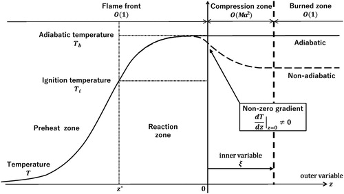
In this study, we assume that the squared Mach number ${Ma}^2$ is sufficiently small. Then, the inner variable, or the stretched variable, ξ is introduced as (11) $z={Ma}^2\xi ({Ma}^2\ll 1),$(11) where ξ represents the coordinate in the compression zone behind a flame front and z is the variable outside the compression zone as shown in Figure 1.

Figure 1. Schematic diagram of regions composed of a flame front and succeeding burned zones. The matching of inner and outer solutions is made in the overlapping region, where compression zone meets burned zone, denoted by vertical dashed line.

All of the quantities are approximated in the form of power series with respect to ${Ma}^2(\ll 1)$ with truncations made at $O\left({Ma}^2\right)$. In the outer regions ($z\le 0,0<z$), (12a) $\begin{array}{rl}R& ={\check{R}}_0+{Ma}^2{\check{R}}_2,V={\check{V}}_0+{Ma}^2{\check{V}}_2,P={\check{P}}_0+{Ma}^2{\check{P}}_2,\end{array}$(12a) (12b) $\begin{array}{rl}T& ={\check{T}}_0+{Ma}^2{\check{T}}_2,Y={\check{Y}}_0+{Ma}^2{\check{Y}}_2,\end{array}$(12b) and in the inner region or the compression region ($0\le \xi <+\mathrm{\infty }$), (13a) $\begin{array}{rl}R& ={\check{\rho }}_0+{Ma}^2{\check{\rho }}_2,V={\check{v}}_0+{Ma}^2{\check{v}}_2,P={\check{p}}_0+{Ma}^2{\check{p}}_2,\end{array}$(13a) (13b) $\begin{array}{rl}T& ={\check{\theta }}_0+{Ma}^2{\check{\theta }}_2,Y={\check{c}}_0+{Ma}^2{\check{c}}_2.\end{array}$(13b) The compressibility effect is represented by $O\left({Ma}^2\right)$ terms.

2.3. Matching conditions

For convenience in the later calculation, we recall the matching conditions between the inner and outer solutions in the overlapping region, where $\xi \to +\mathrm{\infty }$ and $z\to 0+$ as ${Ma}^2\to 0$. Let Φ be any function and its asymptotic expansions with respect to ${Ma}^2$ are assumed to be $\begin{array}{rl}\mathrm{\Phi }& ={\check{\mathrm{\Phi }}}_0\left(z\right)+{Ma}^2{\check{\mathrm{\Phi }}}_2\left(z\right)+O\left({Ma}^4\right)(z\le 0,z>0),\\ \mathrm{\Phi }& ={\check{\phi }}_0\left(\xi \right)+{Ma}^2{\check{\phi }}_2\left(\xi \right)+O\left({Ma}^4\right)(0\le \xi <+\mathrm{\infty }).\end{array}$We assume that the inner and the outer solutions and their derivatives are continuous in the overlapping region or at the burned edge of compression zone. Then, the matching conditions read as [57] (14a) $\begin{array}{rl}{\check{\phi }}_0{|}_{\xi \to +\mathrm{\infty }}& ={\check{\mathrm{\Phi }}}_0{|}_{z\to 0+},{\check{\phi }}_2{|}_{\xi \to +\mathrm{\infty }}={\check{\mathrm{\Phi }}}_2{|}_{z\to 0+}+\xi \frac{\mathrm{d}{\check{\mathrm{\Phi }}}_0}{\mathrm{d}z}{|}_{z\to 0+},\end{array}$(14a) (14b) $\begin{array}{rl}\frac{\mathrm{d}{\check{\phi }}_0}{\mathrm{d}\xi }{|}_{\xi \to +\mathrm{\infty }}& =0,\frac{\mathrm{d}{\check{\phi }}_2}{\mathrm{d}\xi }{|}_{\xi \to +\mathrm{\infty }}=\frac{\mathrm{d}{\check{\mathrm{\Phi }}}_0}{\mathrm{d}z}{|}_{z\to 0+}.\end{array}$(14b) We also assume that all quantities are continuous at $\xi =0$, or z = 0. (15) ${\check{\phi }}_0{|}_{\xi =0}={\check{\mathrm{\Phi }}}_0{|}_{z=0}={\check{\mathrm{\Phi }}}_0{|}_{z\to 0-},{\check{\phi }}_2{|}_{\xi =0}={\check{\mathrm{\Phi }}}_2{|}_{z=0}={\check{\mathrm{\Phi }}}_2{|}_{z\to 0-}.$(15) For simplicity, we will use the following notation. (16a) $\begin{array}{rl}{\check{\mathrm{\Phi }}}_0{|}_{z\to 0-}& ={\check{\mathrm{\Phi }}}_{0-},{\check{\mathrm{\Phi }}}_0{|}_{z\to 0+}={\check{\mathrm{\Phi }}}_{0+},\end{array}$(16a) (16b) $\begin{array}{rl}\frac{\mathrm{d}{\check{\mathrm{\Phi }}}_0}{\mathrm{d}z}{|}_{z\to 0-}& =\frac{\mathrm{d}{\check{\mathrm{\Phi }}}_0}{\mathrm{d}z}{|}_{-},\frac{\mathrm{d}{\check{\mathrm{\Phi }}}_0}{\mathrm{d}z}{|}_{z\to 0+}=\frac{\mathrm{d}{\check{\mathrm{\Phi }}}_0}{\mathrm{d}z}{|}_{+}.\end{array}$(16b) The same things are true for the higher order terms.

3. Compression zone

We investigate the compression zone by use of the matched asymptotic expansions with respect to small squared Mach numbers, ${Ma}^2\ll 1$, and the stretched variable ξ, which is defined by (11(11) $z={Ma}^2\xi ({Ma}^2\ll 1),$(11) ). The compression zone ($0\le \xi <+\mathrm{\infty }$) is located on the burned side of a flame front as shown in Figure 1. We find that the inner solutions in this region are expressed by use of Lambert W function. The smooth decrease of temperature behind a flame front due to gas compression is observed for negative values of inner solution at $O\left({Ma}^2\right)$, ${\check{\theta }}_2$ in (13b(13b) $\begin{array}{rl}T& ={\check{\theta }}_0+{Ma}^2{\check{\theta }}_2,Y={\check{c}}_0+{Ma}^2{\check{c}}_2.\end{array}$(13b) ), for non-zero values of Ma. There is a possibility that the sign of ${\check{\theta }}_2$ becomes positive or negative. This fact is discussed in view of the ignition temperature and the viscosity in Section 5.2. The inner solutions are matched with the outer ones by use of the matching conditions (14(14a) $\begin{array}{rl}{\check{\phi }}_0{|}_{\xi \to +\mathrm{\infty }}& ={\check{\mathrm{\Phi }}}_0{|}_{z\to 0+},{\check{\phi }}_2{|}_{\xi \to +\mathrm{\infty }}={\check{\mathrm{\Phi }}}_2{|}_{z\to 0+}+\xi \frac{\mathrm{d}{\check{\mathrm{\Phi }}}_0}{\mathrm{d}z}{|}_{z\to 0+},\end{array}$(14a) ) and the continuity conditions (15(15) ${\check{\phi }}_0{|}_{\xi =0}={\check{\mathrm{\Phi }}}_0{|}_{z=0}={\check{\mathrm{\Phi }}}_0{|}_{z\to 0-},{\check{\phi }}_2{|}_{\xi =0}={\check{\mathrm{\Phi }}}_2{|}_{z=0}={\check{\mathrm{\Phi }}}_2{|}_{z\to 0-}.$(15) ). Then, we obtain the jump conditions, or the boundary conditions, across the compression zone which are in turn used for calculating the solutions in the outer regions ($z\le 0,z>0$).

3.1. $O\left({Ma}^0\right)$ terms

At first, we seek for the inner solutions at $O\left({Ma}^0\right)$. Substituting (13(13a) $\begin{array}{rl}R& ={\check{\rho }}_0+{Ma}^2{\check{\rho }}_2,V={\check{v}}_0+{Ma}^2{\check{v}}_2,P={\check{p}}_0+{Ma}^2{\check{p}}_2,\end{array}$(13a) ) into (6(6) $\begin{array}{rl}P& =RT,\end{array}$(6) ) and (9(9) $M=RV\equiv 1.$(9) ), we obtain the following equations at $O\left({Ma}^0\right)$. (17) ${\check{p}}_0={\check{\rho }}_0{\check{\theta }}_0,1={\check{\rho }}_0{\check{v}}_0.$(17) These equations will be used to obtain the simple expression of equations in the later calculation. By use of (9(9) $M=RV\equiv 1.$(9) ), the substitution of (13(13a) $\begin{array}{rl}R& ={\check{\rho }}_0+{Ma}^2{\check{\rho }}_2,V={\check{v}}_0+{Ma}^2{\check{v}}_2,P={\check{p}}_0+{Ma}^2{\check{p}}_2,\end{array}$(13a) ) into (4(4) $\begin{array}{rl}M\frac{\mathrm{d}T}{\mathrm{d}z}& =\frac{{\mathrm{d}}^{2}T}{\mathrm{d}{z}^2}+\frac{\gamma -1}{\gamma }V\frac{\mathrm{d}P}{\mathrm{d}z}+\frac{4}{3}(\gamma -1)Pr{Ma}^2{\left(\frac{\mathrm{d}V}{\mathrm{d}z}\right)}^2+qQ,\end{array}$(4) ) and (5(5) $\begin{array}{rl}M\frac{\mathrm{d}Y}{\mathrm{d}z}& =\frac{1}{Le}\frac{{\mathrm{d}}^{2}Y}{\mathrm{d}{z}^2}-Q,\end{array}$(5) ) leads to (18) $0=\frac{{\mathrm{d}}^2{\check{\theta }}_0}{\mathrm{d}{\xi }^2},0=\frac{{\mathrm{d}}^2{\check{c}}_0}{\mathrm{d}{\xi }^2}.$(18) Integrating (18(18) $0=\frac{{\mathrm{d}}^2{\check{\theta }}_0}{\mathrm{d}{\xi }^2},0=\frac{{\mathrm{d}}^2{\check{c}}_0}{\mathrm{d}{\xi }^2}.$(18) ), with the help of the first equation of (14b(14b) $\begin{array}{rl}\frac{\mathrm{d}{\check{\phi }}_0}{\mathrm{d}\xi }{|}_{\xi \to +\mathrm{\infty }}& =0,\frac{\mathrm{d}{\check{\phi }}_2}{\mathrm{d}\xi }{|}_{\xi \to +\mathrm{\infty }}=\frac{\mathrm{d}{\check{\mathrm{\Phi }}}_0}{\mathrm{d}z}{|}_{z\to 0+}.\end{array}$(14b) ), we find that $\mathrm{d}{\check{\theta }}_0/d\xi =d{\check{c}}_0/d\xi =0$. For example, $\text{const.}=\mathrm{d}{\check{\theta }}_0/d\xi =\mathrm{d}{\check{\theta }}_0/d\xi {|}_{\xi \to +\mathrm{\infty }}=0$. Then, we get (19) ${\check{\theta }}_0=\mathrm{c}\mathrm{o}\mathrm{n}\mathrm{s}\mathrm{t}.,{\check{c}}_0=\mathrm{c}\mathrm{o}\mathrm{n}\mathrm{s}\mathrm{t}.$(19) In particular, the value of ${\check{c}}_0$ is determined by (10(10) $Y\equiv 0(z>0).$(10) ) as (20) $\mathrm{c}\mathrm{o}\mathrm{n}\mathrm{s}\mathrm{t}.={\check{c}}_0={\check{c}}_0{|}_{\xi \to +\mathrm{\infty }}={\check{Y}}_0{|}_{z\to +0}=0,$(20) where the first equation of (14a(14a) $\begin{array}{rl}{\check{\phi }}_0{|}_{\xi \to +\mathrm{\infty }}& ={\check{\mathrm{\Phi }}}_0{|}_{z\to 0+},{\check{\phi }}_2{|}_{\xi \to +\mathrm{\infty }}={\check{\mathrm{\Phi }}}_2{|}_{z\to 0+}+\xi \frac{\mathrm{d}{\check{\mathrm{\Phi }}}_0}{\mathrm{d}z}{|}_{z\to 0+},\end{array}$(14a) ) is used in the third equality. From (3(3) $\begin{array}{rl}M\frac{\mathrm{d}V}{\mathrm{d}z}& =-\frac{1}{\gamma {Ma}^2}\frac{\mathrm{d}P}{\mathrm{d}z}+\frac{4}{3}Pr\frac{{\mathrm{d}}^{2}V}{\mathrm{d}{z}^2},\end{array}$(3) ), by use of (9(9) $M=RV\equiv 1.$(9) ) and (13a(13a) $\begin{array}{rl}R& ={\check{\rho }}_0+{Ma}^2{\check{\rho }}_2,V={\check{v}}_0+{Ma}^2{\check{v}}_2,P={\check{p}}_0+{Ma}^2{\check{p}}_2,\end{array}$(13a) ), we have (21) $0=-\frac{\mathrm{d}{\check{p}}_0}{\mathrm{d}\xi }+\nu \frac{{\mathrm{d}}^2{\check{v}}_0}{\mathrm{d}{\xi }^2},$(21) where, for convenience, we put (22) $\nu =\frac{4}{3}\gamma Pr.$(22) Integrating (21(21) $0=-\frac{\mathrm{d}{\check{p}}_0}{\mathrm{d}\xi }+\nu \frac{{\mathrm{d}}^2{\check{v}}_0}{\mathrm{d}{\xi }^2},$(21) ), we get (23) ${\check{p}}_0=\nu \frac{\mathrm{d}{\check{v}}_0}{\mathrm{d}\xi }+{\check{p}}_c,$(23) where ${\check{p}}_c$ is an integral constant. We find that the pressure at $O\left({Ma}^0\right)$, ${\check{p}}_0$, becomes constant if there is no viscous effect, Pr = 0, or $\nu =0$. We are interested in the case of $Pr\ne 0$, for instance, $Pr\approx 3/4$ in air. Therefore, ${\check{p}}_0$ is considered to be not constant in practice. By use of the first equation of (14b(14b) $\begin{array}{rl}\frac{\mathrm{d}{\check{\phi }}_0}{\mathrm{d}\xi }{|}_{\xi \to +\mathrm{\infty }}& =0,\frac{\mathrm{d}{\check{\phi }}_2}{\mathrm{d}\xi }{|}_{\xi \to +\mathrm{\infty }}=\frac{\mathrm{d}{\check{\mathrm{\Phi }}}_0}{\mathrm{d}z}{|}_{z\to 0+}.\end{array}$(14b) ), or $\mathrm{d}{\check{v}}_0/\mathrm{d}\xi \to 0$ as $\xi \to +\mathrm{\infty }$, the integral constant ${\check{p}}_c$ is determined as (24) ${\check{p}}_c={\check{p}}_0{|}_{\xi \to +\mathrm{\infty }}={\check{P}}_0{|}_{z\to 0+}={\check{P}}_{0+},$(24) where the first equation of (14a(14a) $\begin{array}{rl}{\check{\phi }}_0{|}_{\xi \to +\mathrm{\infty }}& ={\check{\mathrm{\Phi }}}_0{|}_{z\to 0+},{\check{\phi }}_2{|}_{\xi \to +\mathrm{\infty }}={\check{\mathrm{\Phi }}}_2{|}_{z\to 0+}+\xi \frac{\mathrm{d}{\check{\mathrm{\Phi }}}_0}{\mathrm{d}z}{|}_{z\to 0+},\end{array}$(14a) ) is employed in the second equality. From (17(17) ${\check{p}}_0={\check{\rho }}_0{\check{\theta }}_0,1={\check{\rho }}_0{\check{v}}_0.$(17) ), in the limit of $\xi \to +\mathrm{\infty }$, we find (25) $1={\check{R}}_{0+}{\check{V}}_{0+},{\check{P}}_{0+}={\check{R}}_{0+}{\check{T}}_{0+}.$(25) Therefore, due to (19(19) ${\check{\theta }}_0=\mathrm{c}\mathrm{o}\mathrm{n}\mathrm{s}\mathrm{t}.,{\check{c}}_0=\mathrm{c}\mathrm{o}\mathrm{n}\mathrm{s}\mathrm{t}.$(19) ), (25(25) $1={\check{R}}_{0+}{\check{V}}_{0+},{\check{P}}_{0+}={\check{R}}_{0+}{\check{T}}_{0+}.$(25) ) gives the following relation. (26) ${\check{\theta }}_0={\check{T}}_{0+}={\check{P}}_{0+}{\check{V}}_{0+}.$(26) Substituting (17(17) ${\check{p}}_0={\check{\rho }}_0{\check{\theta }}_0,1={\check{\rho }}_0{\check{v}}_0.$(17) ) into (23(23) ${\check{p}}_0=\nu \frac{\mathrm{d}{\check{v}}_0}{\mathrm{d}\xi }+{\check{p}}_c,$(23) ), with the help of (26(26) ${\check{\theta }}_0={\check{T}}_{0+}={\check{P}}_{0+}{\check{V}}_{0+}.$(26) ), we obtain the following differential equation for ${\check{v}}_0$ ($\ge 0$). (27) $\frac{{\check{v}}_0}{{\check{v}}_0-{\check{V}}_{0+}}\frac{\mathrm{d}{\check{v}}_0}{\mathrm{d}\xi }=-\frac{{\check{P}}_{0+}}{\nu }.$(27) From (27(27) $\frac{{\check{v}}_0}{{\check{v}}_0-{\check{V}}_{0+}}\frac{\mathrm{d}{\check{v}}_0}{\mathrm{d}\xi }=-\frac{{\check{P}}_{0+}}{\nu }.$(27) ), we readily find that ${\check{v}}_0$ monotonically increases or decreases in the region of $0\le \xi <+\mathrm{\infty }$, because the right hand side of (27(27) $\frac{{\check{v}}_0}{{\check{v}}_0-{\check{V}}_{0+}}\frac{\mathrm{d}{\check{v}}_0}{\mathrm{d}\xi }=-\frac{{\check{P}}_{0+}}{\nu }.$(27) ) is negative constant and $d{\check{v}}_0/d\xi =0$ is possible only when $\xi \to +\mathrm{\infty }$, where ${\check{v}}_0={\check{V}}_{0+}$. Integrating (27(27) $\frac{{\check{v}}_0}{{\check{v}}_0-{\check{V}}_{0+}}\frac{\mathrm{d}{\check{v}}_0}{\mathrm{d}\xi }=-\frac{{\check{P}}_{0+}}{\nu }.$(27) ), we obtain (28) $\ln \left|\frac{{\check{v}}_0}{{\check{V}}_{0+}}-1\right|+\frac{{\check{v}}_0}{{\check{V}}_{0+}}=-\frac{1}{\nu }\frac{{\check{P}}_{0+}}{{\check{V}}_{0+}}\xi +C,$(28) where the integral constant C is determined at $\xi =0$. (29) $\ln \left|\frac{{\check{V}}_{0-}}{{\check{V}}_{0+}}-1\right|+\frac{{\check{V}}_{0-}}{{\check{V}}_{0+}}=C.$(29) We note that the first equation of (15(15) ${\check{\phi }}_0{|}_{\xi =0}={\check{\mathrm{\Phi }}}_0{|}_{z=0}={\check{\mathrm{\Phi }}}_0{|}_{z\to 0-},{\check{\phi }}_2{|}_{\xi =0}={\check{\mathrm{\Phi }}}_2{|}_{z=0}={\check{\mathrm{\Phi }}}_2{|}_{z\to 0-}.$(15) ) is used to find ${\check{v}}_0{|}_{\xi =0}={\check{V}}_0{|}_{z=0}={\check{V}}_{0-}$. Due to the monotonicity of ${\check{v}}_0$, (28(28) $\ln \left|\frac{{\check{v}}_0}{{\check{V}}_{0+}}-1\right|+\frac{{\check{v}}_0}{{\check{V}}_{0+}}=-\frac{1}{\nu }\frac{{\check{P}}_{0+}}{{\check{V}}_{0+}}\xi +C,$(28) ) is rewritten without the absolute value symbol as (30) $\left(\frac{{\check{v}}_0}{{\check{V}}_{0+}}-1\right)\exp \left(\frac{{\check{v}}_0}{{\check{V}}_{0+}}-1\right)=\left(\frac{{\check{V}}_{0-}}{{\check{V}}_{0+}}-1\right)\exp \left(-\frac{1}{\nu }\frac{{\check{P}}_{0+}}{{\check{V}}_{0+}}\xi +\frac{{\check{V}}_{0-}}{{\check{V}}_{0+}}-1\right).$(30) It is possible to solve (30(30) $\left(\frac{{\check{v}}_0}{{\check{V}}_{0+}}-1\right)\exp \left(\frac{{\check{v}}_0}{{\check{V}}_{0+}}-1\right)=\left(\frac{{\check{V}}_{0-}}{{\check{V}}_{0+}}-1\right)\exp \left(-\frac{1}{\nu }\frac{{\check{P}}_{0+}}{{\check{V}}_{0+}}\xi +\frac{{\check{V}}_{0-}}{{\check{V}}_{0+}}-1\right).$(30) ) by use of the Lambert W function.

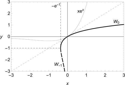
Definition 3.1

Lambert W function

Suppose x and y are real numbers. Then the Lambert W function is defined by two branches of the inverse relation of $y=x\exp \left(x\right)$ as follows. $y=W_0\left(x\right)(x\ge -1/e,y\ge -1),y=W_{-1}\left(x\right)(-1/e\le x<0,y\le -1).$

Figure 2 shows the profile of Lambert W function.

Because ${\check{v}}_0$ is positive, we find ${\check{v}}_0/{\check{V}}_{0+}-1\ge -1$. Therefore, the upper branch $W_0$ of the Lambert W function is employed to obtain the solution of (30(30) $\left(\frac{{\check{v}}_0}{{\check{V}}_{0+}}-1\right)\exp \left(\frac{{\check{v}}_0}{{\check{V}}_{0+}}-1\right)=\left(\frac{{\check{V}}_{0-}}{{\check{V}}_{0+}}-1\right)\exp \left(-\frac{1}{\nu }\frac{{\check{P}}_{0+}}{{\check{V}}_{0+}}\xi +\frac{{\check{V}}_{0-}}{{\check{V}}_{0+}}-1\right).$(30) ). We set (31) $W=W_0\left(g\right(\xi \left)\right),$(31) with (32) $g\left(\xi \right)=\left(\frac{{\check{V}}_{0-}}{{\check{V}}_{0+}}-1\right)\exp \left(-\frac{1}{\nu }\frac{{\check{P}}_{0+}}{{\check{V}}_{0+}}\xi +\frac{{\check{V}}_{0-}}{{\check{V}}_{0+}}-1\right).$(32) Then, we get the solution of (30(30) $\left(\frac{{\check{v}}_0}{{\check{V}}_{0+}}-1\right)\exp \left(\frac{{\check{v}}_0}{{\check{V}}_{0+}}-1\right)=\left(\frac{{\check{V}}_{0-}}{{\check{V}}_{0+}}-1\right)\exp \left(-\frac{1}{\nu }\frac{{\check{P}}_{0+}}{{\check{V}}_{0+}}\xi +\frac{{\check{V}}_{0-}}{{\check{V}}_{0+}}-1\right).$(30) ) as (33) ${\check{v}}_0={\check{V}}_{0+}\left(1+W\right).$(33) Substituting (33(33) ${\check{v}}_0={\check{V}}_{0+}\left(1+W\right).$(33) ) into (23(23) ${\check{p}}_0=\nu \frac{\mathrm{d}{\check{v}}_0}{\mathrm{d}\xi }+{\check{p}}_c,$(23) ), we gain the solution satisfying (23(23) ${\check{p}}_0=\nu \frac{\mathrm{d}{\check{v}}_0}{\mathrm{d}\xi }+{\check{p}}_c,$(23) ) as (34) ${\check{p}}_0=\frac{{\check{P}}_{0+}}{1+W},$(34) where we note that [58] is referred to for the calculation of Lambert W function.

Figure 2. Two branches of Lambert W function in Definition 3.1. They meet each other at $(x,y)=(-1/e,-1)$.

3.2. $O\left({Ma}^2\right)$ terms

Substituting (13(13a) $\begin{array}{rl}R& ={\check{\rho }}_0+{Ma}^2{\check{\rho }}_2,V={\check{v}}_0+{Ma}^2{\check{v}}_2,P={\check{p}}_0+{Ma}^2{\check{p}}_2,\end{array}$(13a) ) into (4(4) $\begin{array}{rl}M\frac{\mathrm{d}T}{\mathrm{d}z}& =\frac{{\mathrm{d}}^{2}T}{\mathrm{d}{z}^2}+\frac{\gamma -1}{\gamma }V\frac{\mathrm{d}P}{\mathrm{d}z}+\frac{4}{3}(\gamma -1)Pr{Ma}^2{\left(\frac{\mathrm{d}V}{\mathrm{d}z}\right)}^2+qQ,\end{array}$(4) ) and (5(5) $\begin{array}{rl}M\frac{\mathrm{d}Y}{\mathrm{d}z}& =\frac{1}{Le}\frac{{\mathrm{d}}^{2}Y}{\mathrm{d}{z}^2}-Q,\end{array}$(5) ), by use of (9(9) $M=RV\equiv 1.$(9) ) and (19(19) ${\check{\theta }}_0=\mathrm{c}\mathrm{o}\mathrm{n}\mathrm{s}\mathrm{t}.,{\check{c}}_0=\mathrm{c}\mathrm{o}\mathrm{n}\mathrm{s}\mathrm{t}.$(19) ), we get the following equations at $O\left({Ma}^2\right)$. (35) $\begin{array}{rl}0& =\frac{{\mathrm{d}}^2{\check{\theta }}_2}{\mathrm{d}{\xi }^2}+\frac{\gamma -1}{\gamma }{\check{v}}_0\frac{\mathrm{d}{\check{p}}_0}{\mathrm{d}\xi }+\frac{4}{3}(\gamma -1)Pr{\left(\frac{\mathrm{d}{\check{v}}_0}{\mathrm{d}\xi }\right)}^2,\end{array}$(35) (36) $\begin{array}{rl}0& =\frac{1}{Le}\frac{{\mathrm{d}}^2{\check{c}}_2}{\mathrm{d}{\xi }^2}.\end{array}$(36) From (10(10) $Y\equiv 0(z>0).$(10) ), by use of (14(14a) $\begin{array}{rl}{\check{\phi }}_0{|}_{\xi \to +\mathrm{\infty }}& ={\check{\mathrm{\Phi }}}_0{|}_{z\to 0+},{\check{\phi }}_2{|}_{\xi \to +\mathrm{\infty }}={\check{\mathrm{\Phi }}}_2{|}_{z\to 0+}+\xi \frac{\mathrm{d}{\check{\mathrm{\Phi }}}_0}{\mathrm{d}z}{|}_{z\to 0+},\end{array}$(14a) ), we readily find the solution of (36(36) $\begin{array}{rl}0& =\frac{1}{Le}\frac{{\mathrm{d}}^2{\check{c}}_2}{\mathrm{d}{\xi }^2}.\end{array}$(36) ) as (37) ${\check{c}}_2=0.$(37) The heat-conduction equation (35(35) $\begin{array}{rl}0& =\frac{{\mathrm{d}}^2{\check{\theta }}_2}{\mathrm{d}{\xi }^2}+\frac{\gamma -1}{\gamma }{\check{v}}_0\frac{\mathrm{d}{\check{p}}_0}{\mathrm{d}\xi }+\frac{4}{3}(\gamma -1)Pr{\left(\frac{\mathrm{d}{\check{v}}_0}{\mathrm{d}\xi }\right)}^2,\end{array}$(35) ) is rewritten, with (33(33) ${\check{v}}_0={\check{V}}_{0+}\left(1+W\right).$(33) ) and (34(34) ${\check{p}}_0=\frac{{\check{P}}_{0+}}{1+W},$(34) ) substituted, as (38) $0=\frac{{\mathrm{d}}^2{\check{\theta }}_2}{\mathrm{d}{\xi }^2}+\frac{\gamma -1}{\gamma }\frac{{\check{P}}_{0+}^2}{\nu }\frac{W}{1+W}.$(38) The integration of (38(38) $0=\frac{{\mathrm{d}}^2{\check{\theta }}_2}{\mathrm{d}{\xi }^2}+\frac{\gamma -1}{\gamma }\frac{{\check{P}}_{0+}^2}{\nu }\frac{W}{1+W}.$(38) ) leads to (39) $C=\frac{\mathrm{d}{\check{\theta }}_2}{\mathrm{d}\xi }-\frac{\gamma -1}{\gamma }{\check{\theta }}_{0}W.$(39) The integral constant C is determined as $C=\mathrm{d}{\check{T}}_0/\mathrm{d}z{|}_{+}$ by employing the matching condition (14b(14b) $\begin{array}{rl}\frac{\mathrm{d}{\check{\phi }}_0}{\mathrm{d}\xi }{|}_{\xi \to +\mathrm{\infty }}& =0,\frac{\mathrm{d}{\check{\phi }}_2}{\mathrm{d}\xi }{|}_{\xi \to +\mathrm{\infty }}=\frac{\mathrm{d}{\check{\mathrm{\Phi }}}_0}{\mathrm{d}z}{|}_{z\to 0+}.\end{array}$(14b) ) as $\xi \to +\mathrm{\infty }$. Then, recalling (26(26) ${\check{\theta }}_0={\check{T}}_{0+}={\check{P}}_{0+}{\check{V}}_{0+}.$(26) ), we integrate (39(39) $C=\frac{\mathrm{d}{\check{\theta }}_2}{\mathrm{d}\xi }-\frac{\gamma -1}{\gamma }{\check{\theta }}_{0}W.$(39) ) as (40) ${\check{\theta }}_2=C^{\prime }+\frac{\mathrm{d}{\check{T}}_0}{\mathrm{d}z}{|}_{+}\xi -\frac{\gamma -1}{\gamma }\nu {\check{V}}_{0+}^{2}W\left(1+\frac{W}{2}\right).$(40) The integral constant $C^{\prime }$ is determined by taking the limit of $\xi \to +\mathrm{\infty }$, with the help of (14a(14a) $\begin{array}{rl}{\check{\phi }}_0{|}_{\xi \to +\mathrm{\infty }}& ={\check{\mathrm{\Phi }}}_0{|}_{z\to 0+},{\check{\phi }}_2{|}_{\xi \to +\mathrm{\infty }}={\check{\mathrm{\Phi }}}_2{|}_{z\to 0+}+\xi \frac{\mathrm{d}{\check{\mathrm{\Phi }}}_0}{\mathrm{d}z}{|}_{z\to 0+},\end{array}$(14a) ), as (41) $C^{\prime }={\check{T}}_{2+}.$(41)

3.3. Inner solutions

From the above calculation, we obtain the solutions in the compression zone as follows. (42a) $\begin{array}{rl}T& ={\check{T}}_{0+}+{Ma}^2\{{\check{T}}_{2+}+\frac{\mathrm{d}{\check{T}}_0}{\mathrm{d}z}{|}_{+}\xi -\frac{\gamma -1}{\gamma }\nu {\check{V}}_{0+}^{2}W\left(1+\frac{W}{2}\right)\}+O\left({Ma}^4\right),\end{array}$(42a) (42b) $\begin{array}{rl}V& ={\check{V}}_{0+}\left(1+W\right)+{Ma}^2{\check{v}}_2+O\left({Ma}^4\right),\end{array}$(42b) (42c) $\begin{array}{rl}P& =\frac{{\check{P}}_{0+}}{1+W}+{Ma}^2{\check{p}}_2+O\left({Ma}^4\right),\end{array}$(42c) (42d) $\begin{array}{rl}R& =V^{-1},Y=O\left({Ma}^4\right),\end{array}$(42d) with W defined by (31(31) $W=W_0\left(g\right(\xi \left)\right),$(31) ). The description of ${\check{v}}_2$ and ${\check{p}}_2$ is somewhat lengthy and their calculation is devoted to Appendix 1.

3.4. Boundary conditions across the compression zone

In Section 4, we calculate outer solutions by integrating governing equations with (12(12a) $\begin{array}{rl}R& ={\check{R}}_0+{Ma}^2{\check{R}}_2,V={\check{V}}_0+{Ma}^2{\check{V}}_2,P={\check{P}}_0+{Ma}^2{\check{P}}_2,\end{array}$(12a) ) substituted. Then, the boundary conditions across the compression zone are necessary to determine integral constants and briefly derived below. At first, taking $\xi =0$ in (33(33) ${\check{v}}_0={\check{V}}_{0+}\left(1+W\right).$(33) ), the following relation is obtained due to (15(15) ${\check{\phi }}_0{|}_{\xi =0}={\check{\mathrm{\Phi }}}_0{|}_{z=0}={\check{\mathrm{\Phi }}}_0{|}_{z\to 0-},{\check{\phi }}_2{|}_{\xi =0}={\check{\mathrm{\Phi }}}_2{|}_{z=0}={\check{\mathrm{\Phi }}}_2{|}_{z\to 0-}.$(15) ), the continuity at z = 0. (43) ${\check{V}}_{0-}={\check{V}}_{0+}\left(1+W_0\left(g\right(0\left)\right)\right).$(43) This is the boundary condition for the velocity at $O\left({Ma}^0\right)$. By use of (43(43) ${\check{V}}_{0-}={\check{V}}_{0+}\left(1+W_0\left(g\right(0\left)\right)\right).$(43) ) with the help of (15(15) ${\check{\phi }}_0{|}_{\xi =0}={\check{\mathrm{\Phi }}}_0{|}_{z=0}={\check{\mathrm{\Phi }}}_0{|}_{z\to 0-},{\check{\phi }}_2{|}_{\xi =0}={\check{\mathrm{\Phi }}}_2{|}_{z=0}={\check{\mathrm{\Phi }}}_2{|}_{z\to 0-}.$(15) ), the following boundary conditions are obtained by setting $\xi =0$ in (19(19) ${\check{\theta }}_0=\mathrm{c}\mathrm{o}\mathrm{n}\mathrm{s}\mathrm{t}.,{\check{c}}_0=\mathrm{c}\mathrm{o}\mathrm{n}\mathrm{s}\mathrm{t}.$(19) ), (34(34) ${\check{p}}_0=\frac{{\check{P}}_{0+}}{1+W},$(34) ), (37(37) ${\check{c}}_2=0.$(37) ), (39(39) $C=\frac{\mathrm{d}{\check{\theta }}_2}{\mathrm{d}\xi }-\frac{\gamma -1}{\gamma }{\check{\theta }}_{0}W.$(39) ) and (40(40) ${\check{\theta }}_2=C^{\prime }+\frac{\mathrm{d}{\check{T}}_0}{\mathrm{d}z}{|}_{+}\xi -\frac{\gamma -1}{\gamma }\nu {\check{V}}_{0+}^{2}W\left(1+\frac{W}{2}\right).$(40) ). (44) $\begin{array}{rl}{\check{T}}_0{|}_{z\to 0-}& ={\check{T}}_0{|}_{z\to 0+},{\check{Y}}_0{|}_{z\to 0-}={\check{Y}}_0{|}_{z\to 0+},\end{array}$(44) (45) $\begin{array}{rl}{\check{P}}_{0+}& =\frac{{\check{V}}_{0-}}{{\check{V}}_{0+}}{\check{P}}_{0-},\end{array}$(45) (46) $\begin{array}{rl}\frac{d{\check{c}}_2}{\mathrm{d}\xi }{|}_{\xi =0}& =0,\end{array}$(46) (47) $\begin{array}{rl}\frac{\mathrm{d}{\check{\theta }}_2}{\mathrm{d}\xi }{|}_{\xi =0}& =\frac{\mathrm{d}{\check{T}}_0}{\mathrm{d}z}{|}_{z\to 0+}+\frac{\gamma -1}{\gamma }{\check{T}}_{0+}\left(\frac{{\check{V}}_{0-}}{{\check{V}}_{0+}}-1\right),\end{array}$(47) (48) $\begin{array}{rl}{\check{T}}_{2+}& ={\check{T}}_{2-}+\frac{1}{2}\frac{\gamma -1}{\gamma }\nu {\check{V}}_{0+}^2\left({\left(\frac{{\check{V}}_{0-}}{{\check{V}}_{0+}}\right)}^2-1\right).\end{array}$(48)

4. Outer regions

In the previous section, we have obtained the inner solutions in the compression zone and the boundary conditions across it. In this section, we seek for the outer solutions in the outer regions of the compression zone, which consist of the preheat, reaction and burned zones as sketched in Figure 1. For the study of preheat and reaction zones located in front of the compression zone, we impose the strong ignition temperature approximation on the reaction term [59–62]. This assumption enables us to obtain exact solutions. The general type of reaction rate, such as the Arrhenius type [64,65], will be investigated in the future work.

Now, the governing equations in the outer regions are written, by the use of (9(9) $M=RV\equiv 1.$(9) ), as (49) $\begin{array}{rl}\gamma \frac{\mathrm{d}V}{\mathrm{d}z}& =-\frac{1}{{Ma}^2}\frac{\mathrm{d}P}{\mathrm{d}z}+\nu \frac{{\mathrm{d}}^{2}V}{\mathrm{d}{z}^2},\end{array}$(49) (50) $\begin{array}{rl}\frac{\mathrm{d}T}{\mathrm{d}z}& =\frac{{\mathrm{d}}^{2}T}{\mathrm{d}{z}^2}+\frac{\gamma -1}{\gamma }V\frac{\mathrm{d}P}{\mathrm{d}z}+\frac{4}{3}(\gamma -1)Pr{Ma}^2{\left(\frac{\mathrm{d}V}{\mathrm{d}z}\right)}^2+qQ,\end{array}$(50) (51) $\begin{array}{rl}\frac{\mathrm{d}Y}{\mathrm{d}z}& =\frac{1}{Le}\frac{{\mathrm{d}}^{2}Y}{\mathrm{d}{z}^2}-Q,\end{array}$(51) (52) $\begin{array}{rl}P& =RT,\end{array}$(52) with (53) $Q=\left\{\begin{array}{ll}0& (z\le z^{\ast },z>0)\\ Q_c& (z^{\ast }<z\le 0)\end{array}\right.,$(53) where $Q_c$ is some given constant [59]. The position $z^{\ast }$ separates the preheat and the reaction zones as shown in Figure 1. It is natural to consider that the derivatives of the temperature and the mass fraction as well as themselves are continuous at $z=z^{\ast }$. Therefore, we impose the following boundary conditions. (54) $\begin{array}{rl}T{|}_{z\to z^{\ast }-}& =T{|}_{z\to z^{\ast }+}=T_i,\frac{\mathrm{d}T}{\mathrm{d}z}{|}_{z\to z^{\ast }-}=\frac{\mathrm{d}T}{\mathrm{d}z}{|}_{z\to z^{\ast }+},\end{array}$(54) (55) $\begin{array}{rl}Y{|}_{z\to z^{\ast }-}& =Y{|}_{z\to z^{\ast }+},\frac{\mathrm{d}Y}{\mathrm{d}z}{|}_{z\to z^{\ast }-}=\frac{\mathrm{d}Y}{\mathrm{d}z}{|}_{z\to z^{\ast }+},\end{array}$(55) where the ignition temperature $T_i$ is defined by (56) $T{|}_{z=z^{\ast }}=T_i={\check{T}}_{i0}\left(\xi \right)+{Ma}^2{\check{T}}_{i2}\left(\xi \right)+O\left({Ma}^4\right).$(56) In this study, the values of ${\check{T}}_{i0}$ and ${\check{T}}_{i2}$ are able to be calculated for the adiabatic case, as will be shown in (89(89a) $\begin{array}{rl}{\check{T}}_{i0ad}& =1+q{Q}_c(1-{\mathrm{e}}^{z^{\ast }}),\end{array}$(89a) ). The non-adiabatic case is investigated by considering the deviation of $T_i$ from its adiabatic value. The removal of the ignition temperature will be studied in the future work, based on the method of large activation energy asymptotics. The present work focuses on the calculation of exact solutions in the outer region on the unburned side.

4.1. Outer solutions at $O\left({Ma}^0\right)$

We seek for solutions of (49(49) $\begin{array}{rl}\gamma \frac{\mathrm{d}V}{\mathrm{d}z}& =-\frac{1}{{Ma}^2}\frac{\mathrm{d}P}{\mathrm{d}z}+\nu \frac{{\mathrm{d}}^{2}V}{\mathrm{d}{z}^2},\end{array}$(49) )–(52(52) $\begin{array}{rl}P& =RT,\end{array}$(52) ) in the form of asymptotic expansions with respect to ${Ma}^2$ as introduced by (12a(12a) $\begin{array}{rl}R& ={\check{R}}_0+{Ma}^2{\check{R}}_2,V={\check{V}}_0+{Ma}^2{\check{V}}_2,P={\check{P}}_0+{Ma}^2{\check{P}}_2,\end{array}$(12a) ) and (12b(12b) $\begin{array}{rl}T& ={\check{T}}_0+{Ma}^2{\check{T}}_2,Y={\check{Y}}_0+{Ma}^2{\check{Y}}_2,\end{array}$(12b) ). At first, from (8(8) $R=V=P=T=Y=1\mathrm{a}\mathrm{s}z\to -\mathrm{\infty }.$(8) ) and (49(49) $\begin{array}{rl}\gamma \frac{\mathrm{d}V}{\mathrm{d}z}& =-\frac{1}{{Ma}^2}\frac{\mathrm{d}P}{\mathrm{d}z}+\nu \frac{{\mathrm{d}}^{2}V}{\mathrm{d}{z}^2},\end{array}$(49) ), we find that the pressure at $O\left({Ma}^0\right)$ is constant. (57) ${\check{P}}_0=\left\{\begin{array}{ll}1& (z\le 0)\\ {\check{P}}_{0+}& (z>0)\end{array}\right..$(57) Because of (57(57) ${\check{P}}_0=\left\{\begin{array}{ll}1& (z\le 0)\\ {\check{P}}_{0+}& (z>0)\end{array}\right..$(57) ), at $O\left({Ma}^0\right)$, (50(50) $\begin{array}{rl}\frac{\mathrm{d}T}{\mathrm{d}z}& =\frac{{\mathrm{d}}^{2}T}{\mathrm{d}{z}^2}+\frac{\gamma -1}{\gamma }V\frac{\mathrm{d}P}{\mathrm{d}z}+\frac{4}{3}(\gamma -1)Pr{Ma}^2{\left(\frac{\mathrm{d}V}{\mathrm{d}z}\right)}^2+qQ,\end{array}$(50) ) becomes (58) $\frac{\mathrm{d}{\check{T}}_0}{\mathrm{d}z}=\frac{{\mathrm{d}}^2{\check{T}}_0}{\mathrm{d}{z}^2}+qQ.$(58) The general solution of (58(58) $\frac{\mathrm{d}{\check{T}}_0}{\mathrm{d}z}=\frac{{\mathrm{d}}^2{\check{T}}_0}{\mathrm{d}{z}^2}+qQ.$(58) ) is given by (59) ${\check{T}}_0=\left\{\begin{array}{ll}{C}_1+C_2{\mathrm{e}}^z& (z\le z^{\ast })\\ C_3+C_4{\mathrm{e}}^z+q{Q}_{c}z& (z^{\ast }<z\le 0)\\ \sigma & (z>0)\end{array}\right.,$(59) where $C_1$, $C_2$, $C_3$ and $C_4$ are integral constants. Because the solution should be bounded in the far field, $z\to +\mathrm{\infty }$, the temperature is constant on the burned side. Especially, σ is the thermal expansion rate defined by (60) $\sigma ={\check{T}}_{0+}.$(60) As mentioned in Section 2, the temperature is non-dimensionalised by use of its value in the far field on the unburned side, $z\to -\mathrm{\infty }$. Therefore, σ is identical with the thermal expansion rate used in the previous works [29,31,33], which is important to understand the intrinsic instability of a flame front, the Darrieus–Landau instability [10]. The non-adiabatic situation, induced by the compressibility, does not restrict the value of σ to its adiabatic one, 1 + q. As will be shown in (66(66) $\begin{array}{rl}\sigma & =1+q{Q}_c(1-z^{\ast })+A{\mathrm{e}}^{-z^{\ast }},\end{array}$(66) ), σ becomes larger or less than 1 + q depending on the heat release, reaction rate and ignition temperature.

The far-field condition (8(8) $R=V=P=T=Y=1\mathrm{a}\mathrm{s}z\to -\mathrm{\infty }.$(8) ) as $z\to -\mathrm{\infty }$ gives (61) $C_1=1.$(61) The boundary conditions, (54(54) $\begin{array}{rl}T{|}_{z\to z^{\ast }-}& =T{|}_{z\to z^{\ast }+}=T_i,\frac{\mathrm{d}T}{\mathrm{d}z}{|}_{z\to z^{\ast }-}=\frac{\mathrm{d}T}{\mathrm{d}z}{|}_{z\to z^{\ast }+},\end{array}$(54) ) at $z=z^{\ast }$ and (44(44) $\begin{array}{rl}{\check{T}}_0{|}_{z\to 0-}& ={\check{T}}_0{|}_{z\to 0+},{\check{Y}}_0{|}_{z\to 0-}={\check{Y}}_0{|}_{z\to 0+},\end{array}$(44) ) across the compression zone, lead to the following relations between integral constants. (62) $\begin{array}{rl}{\check{T}}_{i0}& =1+C_2{\mathrm{e}}^{z^{\ast }}=C_3+C_4{\mathrm{e}}^{z^{\ast }}+q{Q}_c{z}^{\ast },\end{array}$(62) (63) $\begin{array}{rl}{C}_2{\mathrm{e}}^{z^{\ast }}& =C_4{\mathrm{e}}^{z^{\ast }}+q{Q}_c,\end{array}$(63) (64) $\begin{array}{rl}{C}_3+C_4& =\sigma .\end{array}$(64) From (62(62) $\begin{array}{rl}{\check{T}}_{i0}& =1+C_2{\mathrm{e}}^{z^{\ast }}=C_3+C_4{\mathrm{e}}^{z^{\ast }}+q{Q}_c{z}^{\ast },\end{array}$(62) ), (63(63) $\begin{array}{rl}{C}_2{\mathrm{e}}^{z^{\ast }}& =C_4{\mathrm{e}}^{z^{\ast }}+q{Q}_c,\end{array}$(63) ) and (64(64) $\begin{array}{rl}{C}_3+C_4& =\sigma .\end{array}$(64) ), integral constants $C_2$, $C_3$ and $C_4$ and the thermal expansion rate σ are determined as (65) $\begin{array}{rl}{C}_2& =(T_i-1){\mathrm{e}}^{-z^{\ast }},C_3=\sigma -A{\mathrm{e}}^{-z^{\ast }},C_4=A{\mathrm{e}}^{-z^{\ast }},\end{array}$(65) (66) $\begin{array}{rl}\sigma & =1+q{Q}_c(1-z^{\ast })+A{\mathrm{e}}^{-z^{\ast }},\end{array}$(66) where we put (67) $A={\check{T}}_{i0}-1-q{Q}_c.$(67) Taking account of (52(52) $\begin{array}{rl}P& =RT,\end{array}$(52) ) and (57(57) ${\check{P}}_0=\left\{\begin{array}{ll}1& (z\le 0)\\ {\check{P}}_{0+}& (z>0)\end{array}\right..$(57) ), the solutions of other quantities at $O\left({Ma}^0\right)$ and pressure at $O\left({Ma}^2\right)$ are obtained by solving the following equations. (68) $\begin{array}{rl}{\check{R}}_0{\check{V}}_0& =1,{\check{R}}_0{\check{T}}_0=\left\{\begin{array}{ll}1& (z\le 0)\\ {\check{P}}_{0+}& (z>0)\end{array}\right.,\end{array}$(68) (69) $\begin{array}{rl}\frac{\mathrm{d}{\check{Y}}_0}{\mathrm{d}z}& =\frac{1}{Le}\frac{{\mathrm{d}}^2{\check{Y}}_0}{\mathrm{d}{z}^2}-Q,\end{array}$(69) (70) $\begin{array}{rl}\gamma \frac{\mathrm{d}{\check{V}}_0}{\mathrm{d}z}& =-\frac{\mathrm{d}{\check{P}}_2}{\mathrm{d}z}+\nu \frac{{\mathrm{d}}^2{\check{V}}_0}{\mathrm{d}{z}^2}.\end{array}$(70) Boundary conditions (8(8) $R=V=P=T=Y=1\mathrm{a}\mathrm{s}z\to -\mathrm{\infty }.$(8) ), (44(44) $\begin{array}{rl}{\check{T}}_0{|}_{z\to 0-}& ={\check{T}}_0{|}_{z\to 0+},{\check{Y}}_0{|}_{z\to 0-}={\check{Y}}_0{|}_{z\to 0+},\end{array}$(44) ) and (45(45) $\begin{array}{rl}{\check{P}}_{0+}& =\frac{{\check{V}}_{0-}}{{\check{V}}_{0+}}{\check{P}}_{0-},\end{array}$(45) ) are imposed on (68(68) $\begin{array}{rl}{\check{R}}_0{\check{V}}_0& =1,{\check{R}}_0{\check{T}}_0=\left\{\begin{array}{ll}1& (z\le 0)\\ {\check{P}}_{0+}& (z>0)\end{array}\right.,\end{array}$(68) )-(70(70) $\begin{array}{rl}\gamma \frac{\mathrm{d}{\check{V}}_0}{\mathrm{d}z}& =-\frac{\mathrm{d}{\check{P}}_2}{\mathrm{d}z}+\nu \frac{{\mathrm{d}}^2{\check{V}}_0}{\mathrm{d}{z}^2}.\end{array}$(70) ). Then, the solutions in the outer regions are given as follows. (71) $\begin{array}{rl}{\check{T}}_0& =\left\{\begin{array}{ll}1+({\check{T}}_{i0}-1){\mathrm{e}}^{z-z^{\ast }}& (z\le z^{\ast })\\ \sigma +A({\mathrm{e}}^{z-z^{\ast }}-{\mathrm{e}}^{-z^{\ast }})+q{Q}_{c}z& (z^{\ast }<z\le 0)\\ \sigma & (z>0)\end{array}\right.,\end{array}$(71) (72) $\begin{array}{rl}{\check{Y}}_0& =\left\{\begin{array}{ll}1-\left\{\frac{Q_c}{Le}+\left(1-\frac{Q_c}{Le}+Q_c{z}^{\ast }\right){\mathrm{e}}^{Le{z}^{\ast }}\right\}{\mathrm{e}}^{Le(z-z^{\ast })}& (z\le z^{\ast })\\ \left(\frac{Q_c}{Le}-Q_c{z}^{\ast }-1\right)({\mathrm{e}}^{Lez}-1)-Q_{c}z& (z^{\ast }<z\le 0)\\ 0& (z>0)\end{array}\right.,\end{array}$(72) (73) $\begin{array}{rl}{\check{V}}_0& =\left\{\begin{array}{ll}{\check{T}}_0& (z\le 0)\\ {\check{V}}_{0+}& (z>0)\end{array}\right.,\end{array}$(73) (74) $\begin{array}{rl}{\check{R}}_0& =\left\{\begin{array}{ll}{\check{T}}_0^{-1}& (z\le 0)\\ {\check{V}}_{0+}^{-1}& (z>0)\end{array}\right.,\end{array}$(74) (75) $\begin{array}{rl}{\check{P}}_0& =\left\{\begin{array}{ll}1& (z\le 0)\\ \sigma /{\check{V}}_{0+}& (z>0)\end{array}\right.,\end{array}$(75) (76) $\begin{array}{rl}{\check{P}}_2& =\left\{\begin{array}{ll}(\nu -\gamma )({\check{T}}_{i0}-1){\mathrm{e}}^{z-z^{\ast }}& (z\le z^{\ast })\\ (\nu -\gamma )\left\{q{Q}_c+A{\mathrm{e}}^{z-z^{\ast }}\right\}-\gamma q{Q}_c(z-z^{\ast })& (z^{\ast }<z\le 0)\\ {\check{P}}_{2+}& (z>0)\end{array}\right..\end{array}$(76) In order to determine the unknown parameters $z^{\ast }$ and ${\check{V}}_{0+}$, the additional assumptions on the continuity of gradient of temperature and mass fraction at $\xi =0$, or z = 0, are imposed as the boundary conditions. (77) $\frac{1}{{Ma}^2}\frac{\mathrm{d}\check{T}\left(\xi \right)}{\mathrm{d}\xi }{|}_{\xi =0}=\frac{\mathrm{d}\check{T}\left(z\right)}{\mathrm{d}z}{|}_{z=0},\frac{1}{{Ma}^2}\frac{\mathrm{d}\check{Y}\left(\xi \right)}{\mathrm{d}\xi }{|}_{\xi =0}=\frac{\mathrm{d}\check{Y}\left(z\right)}{\mathrm{d}z}{|}_{z=0}.$(77) Then, at $O\left({Ma}^0\right)$ and $O\left({Ma}^2\right)$, we find (78) $\begin{array}{rl}\frac{\mathrm{d}{\check{\theta }}_0}{\mathrm{d}\xi }{|}_{\xi =0}& =\frac{\mathrm{d}{\check{c}}_0}{\mathrm{d}\xi }{|}_{\xi =0}=0,\end{array}$(78) (79) $\begin{array}{rl}\frac{\mathrm{d}{\check{\theta }}_2}{\mathrm{d}\xi }{|}_{\xi =0}& =\frac{\mathrm{d}{\check{T}}_0}{\mathrm{d}z}{|}_{z=0},0=\frac{\mathrm{d}{\check{c}}_2}{\mathrm{d}\xi }{|}_{\xi =0}=\frac{\mathrm{d}{\check{Y}}_0}{\mathrm{d}z}{|}_{z=0}.\end{array}$(79) The equality in (78(78) $\begin{array}{rl}\frac{\mathrm{d}{\check{\theta }}_0}{\mathrm{d}\xi }{|}_{\xi =0}& =\frac{\mathrm{d}{\check{c}}_0}{\mathrm{d}\xi }{|}_{\xi =0}=0,\end{array}$(78) ) is satisfied by inner solutions (19(19) ${\check{\theta }}_0=\mathrm{c}\mathrm{o}\mathrm{n}\mathrm{s}\mathrm{t}.,{\check{c}}_0=\mathrm{c}\mathrm{o}\mathrm{n}\mathrm{s}\mathrm{t}.$(19) ). The first equality of second equation in (79(79) $\begin{array}{rl}\frac{\mathrm{d}{\check{\theta }}_2}{\mathrm{d}\xi }{|}_{\xi =0}& =\frac{\mathrm{d}{\check{T}}_0}{\mathrm{d}z}{|}_{z=0},0=\frac{\mathrm{d}{\check{c}}_2}{\mathrm{d}\xi }{|}_{\xi =0}=\frac{\mathrm{d}{\check{Y}}_0}{\mathrm{d}z}{|}_{z=0}.\end{array}$(79) ) is due to (46(46) $\begin{array}{rl}\frac{d{\check{c}}_2}{\mathrm{d}\xi }{|}_{\xi =0}& =0,\end{array}$(46) ) and this relation determines $z^{\ast }$, which is the position dividing the preheat and reaction zones, by the use of (72(72) $\begin{array}{rl}{\check{Y}}_0& =\left\{\begin{array}{ll}1-\left\{\frac{Q_c}{Le}+\left(1-\frac{Q_c}{Le}+Q_c{z}^{\ast }\right){\mathrm{e}}^{Le{z}^{\ast }}\right\}{\mathrm{e}}^{Le(z-z^{\ast })}& (z\le z^{\ast })\\ \left(\frac{Q_c}{Le}-Q_c{z}^{\ast }-1\right)({\mathrm{e}}^{Lez}-1)-Q_{c}z& (z^{\ast }<z\le 0)\\ 0& (z>0)\end{array}\right.,\end{array}$(72) ), as (80) $z^{\ast }=-1/Q_c.$(80) It is clear that the increase of the value of $Q_c$ results in the decrease of width of the reaction zone, $|z^{\ast }|$. Figure 1 may help to recognise the reaction zone. This relation is further discussed in relation to the increase or decrease of temperature in Section 5. On the other hand, the decrease of $Q_c$ leads to the large width of the reaction zone without limit. This cold boundary difficulty is due to the constancy of $Q_c$. The resolution of this difficulty will be treated in the future study by considering the temperature dependence of $Q_c$, such as the Arrhenius type, according to the previous works [64,65].

Calculating the gradient of the outer solution of temperature (71(71) $\begin{array}{rl}{\check{T}}_0& =\left\{\begin{array}{ll}1+({\check{T}}_{i0}-1){\mathrm{e}}^{z-z^{\ast }}& (z\le z^{\ast })\\ \sigma +A({\mathrm{e}}^{z-z^{\ast }}-{\mathrm{e}}^{-z^{\ast }})+q{Q}_{c}z& (z^{\ast }<z\le 0)\\ \sigma & (z>0)\end{array}\right.,\end{array}$(71) ), with the help of (80(80) $z^{\ast }=-1/Q_c.$(80) ), we obtain the non-zero condition of temperature gradient at the edge of a flame front on the burned side. (81) $\frac{\mathrm{d}{\check{T}}_0}{\mathrm{d}z}{|}_{-}=\sigma -(1+q).$(81) This condition simply shows that the non-adiabatic profile of a flame front is achieved for the non-adiabatic value of thermal expansion rate, $\sigma \ne 1+q$. The first equation of (79(79) $\begin{array}{rl}\frac{\mathrm{d}{\check{\theta }}_2}{\mathrm{d}\xi }{|}_{\xi =0}& =\frac{\mathrm{d}{\check{T}}_0}{\mathrm{d}z}{|}_{z=0},0=\frac{\mathrm{d}{\check{c}}_2}{\mathrm{d}\xi }{|}_{\xi =0}=\frac{\mathrm{d}{\check{Y}}_0}{\mathrm{d}z}{|}_{z=0}.\end{array}$(79) ) gives the following boundary condition by use of (47(47) $\begin{array}{rl}\frac{\mathrm{d}{\check{\theta }}_2}{\mathrm{d}\xi }{|}_{\xi =0}& =\frac{\mathrm{d}{\check{T}}_0}{\mathrm{d}z}{|}_{z\to 0+}+\frac{\gamma -1}{\gamma }{\check{T}}_{0+}\left(\frac{{\check{V}}_{0-}}{{\check{V}}_{0+}}-1\right),\end{array}$(47) ) and (60(60) $\sigma ={\check{T}}_{0+}.$(60) ). (82) $\frac{\mathrm{d}{\check{T}}_0}{\mathrm{d}z}{|}_{z\to 0-}=\frac{\mathrm{d}{\check{T}}_0}{\mathrm{d}z}{|}_{z\to 0+}+\frac{\gamma -1}{\gamma }\sigma \left(\frac{{\check{V}}_{0-}}{{\check{V}}_{0+}}-1\right).$(82) Substituting (71(71) $\begin{array}{rl}{\check{T}}_0& =\left\{\begin{array}{ll}1+({\check{T}}_{i0}-1){\mathrm{e}}^{z-z^{\ast }}& (z\le z^{\ast })\\ \sigma +A({\mathrm{e}}^{z-z^{\ast }}-{\mathrm{e}}^{-z^{\ast }})+q{Q}_{c}z& (z^{\ast }<z\le 0)\\ \sigma & (z>0)\end{array}\right.,\end{array}$(71) ) into (82(82) $\frac{\mathrm{d}{\check{T}}_0}{\mathrm{d}z}{|}_{z\to 0-}=\frac{\mathrm{d}{\check{T}}_0}{\mathrm{d}z}{|}_{z\to 0+}+\frac{\gamma -1}{\gamma }\sigma \left(\frac{{\check{V}}_{0-}}{{\check{V}}_{0+}}-1\right).$(82) ), we find that the velocity in the burned region, ${\check{V}}_{0+}$, is expressed by use of the thermal expansion rate as follows. (83) ${\check{V}}_{0+}=\frac{(\gamma -1){\sigma }^2}{(2\gamma -1)\sigma -\gamma (1+q)}.$(83)

4.2. Outer solutions at $O\left({Ma}^2\right)$

As for the temperature in the compression zone, the deviation from its adiabatic value is achieved by $O\left({Ma}^2\right)$ term, ${\check{\theta }}_2$, as shown in Section 3. Therefore, we need to calculate the solution of temperature at $O\left({Ma}^2\right)$, ${\check{T}}_2$, in the outer regions, unburned side $z\le 0$ and burned side z>0, to connect the outer and inner solutions for non-zero values of Mach number.

Boundary conditions (8(8) $R=V=P=T=Y=1\mathrm{a}\mathrm{s}z\to -\mathrm{\infty }.$(8) ) and (54(54) $\begin{array}{rl}T{|}_{z\to z^{\ast }-}& =T{|}_{z\to z^{\ast }+}=T_i,\frac{\mathrm{d}T}{\mathrm{d}z}{|}_{z\to z^{\ast }-}=\frac{\mathrm{d}T}{\mathrm{d}z}{|}_{z\to z^{\ast }+},\end{array}$(54) ) are imposed to solve the following equation with ${\check{P}}_2$ substituted from (76(76) $\begin{array}{rl}{\check{P}}_2& =\left\{\begin{array}{ll}(\nu -\gamma )({\check{T}}_{i0}-1){\mathrm{e}}^{z-z^{\ast }}& (z\le z^{\ast })\\ (\nu -\gamma )\left\{q{Q}_c+A{\mathrm{e}}^{z-z^{\ast }}\right\}-\gamma q{Q}_c(z-z^{\ast })& (z^{\ast }<z\le 0)\\ {\check{P}}_{2+}& (z>0)\end{array}\right..\end{array}$(76) ). (84) $\frac{\mathrm{d}{\check{T}}_2}{\mathrm{d}z}=\frac{{\mathrm{d}}^2{\check{T}}_2}{\mathrm{d}{z}^2}+\frac{\gamma -1}{\gamma }{\check{V}}_0\frac{\mathrm{d}{\check{P}}_2}{\mathrm{d}z}+\frac{4}{3}(\gamma -1)Pr{\left(\frac{\mathrm{d}{\check{V}}_0}{\mathrm{d}z}\right)}^2.$(84) Then, the solution of temperature at $O\left({Ma}^2\right)$ is calculated as (85) ${\check{T}}_2=\left\{\begin{array}{ll}{\check{T}}_{i2}{\mathrm{e}}^{z-z^{\ast }}+F\left(z\right){\mathrm{e}}^{z-z^{\ast }}& (z\le z^{\ast })\\ {\check{T}}_{2-}{\mathrm{e}}^z+G\left(z\right)& (z^{\ast }<z\le 0)\\ {\check{T}}_{2+}& (z>0)\end{array}\right.,$(85) with $\begin{array}{rl}F\left(z\right)& =({\check{T}}_{i0}-1)\left(({\check{T}}_{i0}-1)\left(B+\frac{\gamma -1}{2}\right)(1-{\mathrm{e}}^{z-z^{\ast }})-B(z-z^{\ast })\right),\\ G\left(z\right)& =({\check{T}}_{i0}-1)\left(({\check{T}}_{i0}-1)\left(B+\frac{\gamma -1}{2}\right)+B\right)C\\ & +q{Q}_c\left(q{Q}_{c}B-(\gamma -1)\left(\sigma -A{\mathrm{e}}^{-z^{\ast }}\right)\right)(z+(1-z^{\ast }\left)C\right)\\ & -(\gamma -1)q^2{Q}_c^2\left(\frac{z^2}{2}+z^{\ast }\left(1-\frac{z^{\ast }}{2}\right)C\right)-A^2\left(B+\frac{\gamma -1}{2}\right)C(1-{\mathrm{e}}^{z-2z^{\ast }})\\ & -A\left(\frac{\gamma -1}{\gamma }\nu q{Q}_c+B(\sigma -A{\mathrm{e}}^{-z^{\ast }})\right)\left(C+z{\mathrm{e}}^{z-z^{\ast }}\right)-ABq{Q}_c\left(z^{\ast }C+\frac{z^2}{2}{\mathrm{e}}^{z-z^{\ast }}\right),\\ B& =\frac{\gamma -1}{\gamma }(\nu -\gamma ),\\ C\left(z\right)& =1-{\mathrm{e}}^z,\end{array}$where A is defined in (67(67) $A={\check{T}}_{i0}-1-q{Q}_c.$(67) ) and the value of ${\check{T}}_{2-}={\check{T}}_2{|}_{z=0}$ is determined as (86) $\begin{array}{rl}{\check{T}}_{2-}& ={\check{T}}_{i2}{\mathrm{e}}^{-z^{\ast }}+({\check{T}}_{i0}-1)\left(({\check{T}}_{i0}-1)\left(B+\frac{\gamma -1}{2}\right)+B\right)(1-{\mathrm{e}}^{-z^{\ast }})\\ & +q{Q}_c\left(q{Q}_{c}B-(\gamma -1)\left(\sigma -A{\mathrm{e}}^{-z^{\ast }}\right)\right)(1-z^{\ast }-{\mathrm{e}}^{-z^{\ast }})\\ & -(\gamma -1)q^2{Q}_c^2\left(z^{\ast }\left(1-{\mathrm{e}}^{-z^{\ast }}\right)-\frac{{z^{\ast }}^2}{2}\right)-A^2\left(B+\frac{\gamma -1}{2}\right)(1-{\mathrm{e}}^{-z^{\ast }}{)}^2\\ & -A\left(\frac{\gamma -1}{\gamma }\nu q{Q}_c+B(\sigma -A{\mathrm{e}}^{-z^{\ast }})\right)\left(1-(1+z^{\ast }){\mathrm{e}}^{-z^{\ast }}\right)\\ & -ABq{Q}_c\left(z^{\ast }(1-{\mathrm{e}}^{-z^{\ast }})-\frac{{z^{\ast }}^2}{2}{\mathrm{e}}^{-z^{\ast }}\right).\end{array}$(86) The solution of velocity at $O\left({Ma}^2\right)$ is calculated by collecting $O\left({Ma}^2\right)$ terms in (9(9) $M=RV\equiv 1.$(9) ) and (52(52) $\begin{array}{rl}P& =RT,\end{array}$(52) ) with (13(13a) $\begin{array}{rl}R& ={\check{\rho }}_0+{Ma}^2{\check{\rho }}_2,V={\check{v}}_0+{Ma}^2{\check{v}}_2,P={\check{p}}_0+{Ma}^2{\check{p}}_2,\end{array}$(13a) ) substituted. (87) $0={\check{R}}_2{\check{V}}_0+{\check{R}}_0{\check{V}}_2,{\check{P}}_2={\check{R}}_2{\check{T}}_0+{\check{R}}_0{\check{T}}_2.$(87) By eliminating ${\check{R}}_2$ from the above equations, we obtain (88) ${\check{V}}_2=\frac{{\check{T}}_2}{{\check{P}}_0}-\frac{{\check{V}}_0}{{\check{P}}_0}{\check{P}}_2.$(88)

5. Main results

Thanks to the non-zero condition of temperature gradient (82(82) $\frac{\mathrm{d}{\check{T}}_0}{\mathrm{d}z}{|}_{z\to 0-}=\frac{\mathrm{d}{\check{T}}_0}{\mathrm{d}z}{|}_{z\to 0+}+\frac{\gamma -1}{\gamma }\sigma \left(\frac{{\check{V}}_{0-}}{{\check{V}}_{0+}}-1\right).$(82) ), we are able to capture the non-adiabatic profile of a premixed flame front, for example, the decrease of temperature on the burned side. Unlike previous works [24,65,66], this temperature decrease does not come from the volumetric heat loss described by Newton's law of cooling. Instead, our result is due to the pure gas compression effect. For example, the calculation in Section 3.2 clearly indicates the influence of pressure and dissipation on the temperature. Then, the thermal expansion rate σ is different from its adiabatic value, 1 + q, as shown in (66(66) $\begin{array}{rl}\sigma & =1+q{Q}_c(1-z^{\ast })+A{\mathrm{e}}^{-z^{\ast }},\end{array}$(66) ). The extent of its deviation depends on the value of ignition temperature $T_i$ at $O\left({Ma}^0\right)$, which is included in A defined by (67(67) $A={\check{T}}_{i0}-1-q{Q}_c.$(67) ).

The non-monotonic behaviour of temperature due to compressibility effect is achieved by the ignition temperature less than its adiabatic value. In this case, the temperature takes its maximum value inside the reaction zone and decreases on the burned side of a flame front. The similar tendency of temperature has been obtained in the numerical simulation for the SN Ia in the deflagration model [47], in the detonation model [51,52] and in the reconstruction model [53]. It is also interesting to find that the ignition temperature beyond its adiabatic value brings about the monotonic increase of the temperature with its maximum value larger than adiabatic one. Such a temperature profile has been obtained by the numerical computation for a one-dimensional planar flame in view of ignition temperature [67]. Although we have no actual experimental data of spatial temperature distribution to be compared, it is possible to compare our results qualitatively with those in numerical simulation mentioned above and there seems to be no contradiction between them as confirmed in Section 5.2. At first, we recall the adiabatic case. Then, we compare it with the non-adiabatic cases, $T_i<T_{iad}$ and $T_i>T_{iad}$.

5.1. Adiabatic case or zero-temperature gradient

The adiabatic case is recovered by imposing the condition of zero gradient of temperature at the burned edge of a flame front, $dT/dz{|}_{-}=0$. This condition always holds for inviscid flow as confirmed from (31(31) $W=W_0\left(g\right(\xi \left)\right),$(31) ), which gives W = 0 for $\nu =0$: then ${\check{V}}_{0-}={\check{V}}_{0+}$ and (82(82) $\frac{\mathrm{d}{\check{T}}_0}{\mathrm{d}z}{|}_{z\to 0-}=\frac{\mathrm{d}{\check{T}}_0}{\mathrm{d}z}{|}_{z\to 0+}+\frac{\gamma -1}{\gamma }\sigma \left(\frac{{\check{V}}_{0-}}{{\check{V}}_{0+}}-1\right).$(82) ) implies $dT/dz{|}_{-}=0$. In this case, from (81(81) $\frac{\mathrm{d}{\check{T}}_0}{\mathrm{d}z}{|}_{-}=\sigma -(1+q).$(81) ), the thermal expansion rate takes the adiabatic value, $\sigma =1+q$. The ignition temperature in the adiabatic case, denoted by $T_{iad}={\check{T}}_{i0ad}+{Ma}^2{\check{T}}_{i2ad}$, is determined from $d{\check{T}}_0/dz{|}_{-}=0$ and $d{\check{T}}_2/dz{|}_{-}=0$, with (66(66) $\begin{array}{rl}\sigma & =1+q{Q}_c(1-z^{\ast })+A{\mathrm{e}}^{-z^{\ast }},\end{array}$(66) ), (71(71) $\begin{array}{rl}{\check{T}}_0& =\left\{\begin{array}{ll}1+({\check{T}}_{i0}-1){\mathrm{e}}^{z-z^{\ast }}& (z\le z^{\ast })\\ \sigma +A({\mathrm{e}}^{z-z^{\ast }}-{\mathrm{e}}^{-z^{\ast }})+q{Q}_{c}z& (z^{\ast }<z\le 0)\\ \sigma & (z>0)\end{array}\right.,\end{array}$(71) ) and (85(85) ${\check{T}}_2=\left\{\begin{array}{ll}{\check{T}}_{i2}{\mathrm{e}}^{z-z^{\ast }}+F\left(z\right){\mathrm{e}}^{z-z^{\ast }}& (z\le z^{\ast })\\ {\check{T}}_{2-}{\mathrm{e}}^z+G\left(z\right)& (z^{\ast }<z\le 0)\\ {\check{T}}_{2+}& (z>0)\end{array}\right.,$(85) ) substituted, as (89a) $\begin{array}{rl}{\check{T}}_{i0ad}& =1+q{Q}_c(1-{\mathrm{e}}^{z^{\ast }}),\end{array}$(89a) (89b) $\begin{array}{rl}{\check{T}}_{i2ad}& =({\check{T}}_{i0}-1)\left(({\check{T}}_{i0}-1)\left(B+\frac{\gamma -1}{2}\right)+B\right)-(\gamma -1)q^2{Q}_c^2{z}^{\ast }\\ & -q{Q}_c\left(q{Q}_{c}B-(\gamma -1)\left(\sigma -A{\mathrm{e}}^{-z^{\ast }}\right)\right)({\mathrm{e}}^{z^{\ast }}-1)-ABq{Q}_c{z}^{\ast }\left(1+\frac{z^{\ast }}{2}\right)\\ & -A^2(2B+\gamma -1)(1-{\mathrm{e}}^{-z^{\ast }})-A\left(\frac{\gamma -1}{\gamma }\nu q{Q}_c+B(\sigma -A{\mathrm{e}}^{-z^{\ast }})\right)z^{\ast }.\end{array}$(89b)

According to (83(83) ${\check{V}}_{0+}=\frac{(\gamma -1){\sigma }^2}{(2\gamma -1)\sigma -\gamma (1+q)}.$(83) ), when σ takes the adiabatic value 1 + q, the velocity also takes the same value, ${\check{V}}_{0+}=1+q$. This is the adiabatic profile of a premixed flame front. By use of the solutions (42a(42a) $\begin{array}{rl}T& ={\check{T}}_{0+}+{Ma}^2\{{\check{T}}_{2+}+\frac{\mathrm{d}{\check{T}}_0}{\mathrm{d}z}{|}_{+}\xi -\frac{\gamma -1}{\gamma }\nu {\check{V}}_{0+}^{2}W\left(1+\frac{W}{2}\right)\}+O\left({Ma}^4\right),\end{array}$(42a) ), (71(71) $\begin{array}{rl}{\check{T}}_0& =\left\{\begin{array}{ll}1+({\check{T}}_{i0}-1){\mathrm{e}}^{z-z^{\ast }}& (z\le z^{\ast })\\ \sigma +A({\mathrm{e}}^{z-z^{\ast }}-{\mathrm{e}}^{-z^{\ast }})+q{Q}_{c}z& (z^{\ast }<z\le 0)\\ \sigma & (z>0)\end{array}\right.,\end{array}$(71) ) and (85(85) ${\check{T}}_2=\left\{\begin{array}{ll}{\check{T}}_{i2}{\mathrm{e}}^{z-z^{\ast }}+F\left(z\right){\mathrm{e}}^{z-z^{\ast }}& (z\le z^{\ast })\\ {\check{T}}_{2-}{\mathrm{e}}^z+G\left(z\right)& (z^{\ast }<z\le 0)\\ {\check{T}}_{2+}& (z>0)\end{array}\right.,$(85) ), the temperature distribution in the adiabatic case is plotted in Figures 3 and 4 for q = 6, $Q_c=1$ and $\gamma =1.4$. 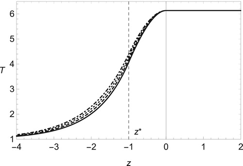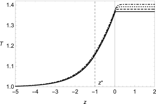From Figure 3, we find that the compressibility effect, or the finite value of Mach number Ma, tends to decrease the temperature below its adiabatic value, 1 + q. The viscous effect, denoted by Prandtl number Pr, raises the temperature inside the flame front but does not change it on the burned side for non-zero values of Ma as shown in Figure 4.

Figure 3. Temperature distribution in adiabatic case, $T_i=T_{iad}$, for several values of Mach number, Ma = 0 (solid line), 0.1 (dashed), 0.2 (dotted) and 0.3 (dot-dashed), with q = 6, $Q_c=1$, $\gamma =1.4$ and Pr = 0.

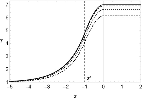
Figure 4. The same as Figure 3 but for fixed Mach number Ma = 0.3 and several Prandtl numbers, Pr = 0 (solid line), 1/4 (dashed), 2/4 (dotted) and 3/4 (dot-dashed).

In the case of $Ma\to 0$, we note that the increase of $T_{iad}={\check{T}}_{i0ad}$ means that of temperature in the reaction and burned zones, as indicated by (66(66) $\begin{array}{rl}\sigma & =1+q{Q}_c(1-z^{\ast })+A{\mathrm{e}}^{-z^{\ast }},\end{array}$(66) ), (67(67) $A={\check{T}}_{i0}-1-q{Q}_c.$(67) ) and (71(71) $\begin{array}{rl}{\check{T}}_0& =\left\{\begin{array}{ll}1+({\check{T}}_{i0}-1){\mathrm{e}}^{z-z^{\ast }}& (z\le z^{\ast })\\ \sigma +A({\mathrm{e}}^{z-z^{\ast }}-{\mathrm{e}}^{-z^{\ast }})+q{Q}_{c}z& (z^{\ast }<z\le 0)\\ \sigma & (z>0)\end{array}\right.,\end{array}$(71) ). Therefore, from (89a(89a) $\begin{array}{rl}{\check{T}}_{i0ad}& =1+q{Q}_c(1-{\mathrm{e}}^{z^{\ast }}),\end{array}$(89a) ), the rise of $Q_c$ implies both the increase of flame temperature and the decrease of width of reaction zone $z^{\ast }$ given by (80(80) $z^{\ast }=-1/Q_c.$(80) ). This relation is in accordance with the statement of previous works [21,63].

5.2. Non-adiabatic cases or non-zero-temperature gradients

We study the non-adiabatic cases by trying out several values of ignition temperature $T_i$ deviating from its adiabatic value $T_{iad}$ given by (89(89a) $\begin{array}{rl}{\check{T}}_{i0ad}& =1+q{Q}_c(1-{\mathrm{e}}^{z^{\ast }}),\end{array}$(89a) ). At first, we study the non-monotonic and monotonic behaviour of temperature by considering two cases, $T_i<T_{iad}$ and $T_i>T_{iad}$ for q = 6, $Q_c=1$ and $\gamma =1.4$. We also investigate the case of $T_i\ne T_{iad}$ for small heat release, q = 0.1. At last, we examine whether the compressibility effect increases or decreases the temperature in view of the ignition temperature, heat release and Prandtl number.

In the case of $T_i<T_{iad}$, we observe the non-monotonic behaviour of temperature as shown in Figures 5 and 6. The temperature takes its maximum value inside the reaction zone and begins to decrease as z increases. This tendency of temperature qualitatively coincides with that obtained by the numerical simulation for the SN Ia in previous works [47,51–53]. The negative gradient of temperature at the edge of a flame front on the burned side is checked by (81(81) $\frac{\mathrm{d}{\check{T}}_0}{\mathrm{d}z}{|}_{-}=\sigma -(1+q).$(81) ) with the help of (66(66) $\begin{array}{rl}\sigma & =1+q{Q}_c(1-z^{\ast })+A{\mathrm{e}}^{-z^{\ast }},\end{array}$(66) ) and (67(67) $A={\check{T}}_{i0}-1-q{Q}_c.$(67) ): that is, $\sigma <1+q$. The non-adiabatic feature of temperature is greatly influenced by the viscosity, represented by the Prandtl number Pr, as shown in Figure 6. Although the viscosity increases the temperature in the preheat zone, it reduces the peak value of temperature in the reaction zone. In Figures 5 and 6, the sharp drop of temperature on the burned side is due to the negative value of ${\check{T}}_{2+}$, which is the solution at $O\left({Ma}^2\right)$, as shown in (85(85) ${\check{T}}_2=\left\{\begin{array}{ll}{\check{T}}_{i2}{\mathrm{e}}^{z-z^{\ast }}+F\left(z\right){\mathrm{e}}^{z-z^{\ast }}& (z\le z^{\ast })\\ {\check{T}}_{2-}{\mathrm{e}}^z+G\left(z\right)& (z^{\ast }<z\le 0)\\ {\check{T}}_{2+}& (z>0)\end{array}\right.,$(85) ). Some calculated values of ${\check{T}}_{2+}$ are listed in Table A1 in Appendix 2. For $T_i<T_{iad}$, we find that the effect of gas compressibility on the decrease of temperature in compression zone is enhanced by the viscosity, though the opposite effect is observed in the most region of flame front.

Figure 5. Temperature distribution in non-adiabatic case, ${\check{T}}_{i0}={\check{T}}_{i0ad}-0.3$ and ${\check{T}}_{i2}={\check{T}}_{i2ad}$, for several values of Mach number, Ma = 0 (solid line), 0.1 (dashed), 0.2 (dotted) and 0.3 (dot-dashed), with q = 6, $Q_c=1$, $\gamma =1.4$ and $Pr=3/4$.

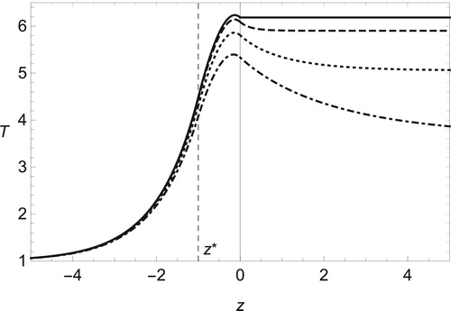
Figure 6. The same as Figure 5 but for fixed value of Mach number Ma = 0.3 with $Pr=1/4$ (solid line), 2/4 (dashed), 3/4 (dotted) and 1 (dot-dashed).

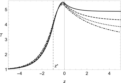
Next, we consider the case of $T_i>T_{iad}$. Then, (81(81) $\frac{\mathrm{d}{\check{T}}_0}{\mathrm{d}z}{|}_{-}=\sigma -(1+q).$(81) ) gives positive value of temperature gradient. The inner and outer solutions give the monotonic increase of temperature as shown in Figures 7 and 8 for q = 6 and $Q_c=1$ and in Figures 9 and 10 for q = 0.1 and $Q_c=0.5$. Although the temperature profile is similar to that of adiabatic case, the temperature on the burned side is larger than the adiabatic one, $T_{ad}=1+q$. The rise of flame temperature due to that of ignition temperature has been shown numerically, for example, in [67]. Comparing Figures 7 and 9, we find that the compressibility brings different aspects of temperature behaviour depending on values of heat release q. For some moderate value of q, the temperature decreases as the Mach number increases as shown in Figure 7. On the other hand, from Figure 9, if q is small enough, the temperature is raised by the compressibility. As indicated in Figures 8 and 10, the viscous effect leads to the increase of temperature in the entire region. We find that the heat release has an significant influence on whether the temperature increases or decreases.

Figure 7. Temperature distribution in non-adiabatic case, ${\check{T}}_{i0}={\check{T}}_{i0ad}+0.3$ and ${\check{T}}_{i2}={\check{T}}_{i2ad}$, for several values of Mach number, Ma = 0 (solid line), 0.1 (dashed), 0.2 (dotted) and 0.3 (dot-dashed), with q = 6, $Q_c=1$, $\gamma =1.4$ and $Pr=3/4$.

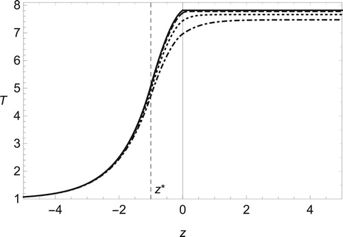
Figure 8. The same as Figure 7 but for fixed value of Mach number Ma = 0.3 with $Pr=1/4$ (solid line), 2/4 (dashed), 3/4 (dotted) and 1 (dot-dashed).

Figure 9. Temperature distribution in non-adiabatic case, ${\check{T}}_{i0}={\check{T}}_{i0ad}+0.1$ and ${\check{T}}_{i2}={\check{T}}_{i2ad}$, for several values of Mach number, Ma = 0 (solid line), 0.1 (dashed), 0.2 (dotted) and 0.3 (dot-dashed), with q = 0.1, $Q_c=1$, $\gamma =1.4$ and $Pr=3/4$.

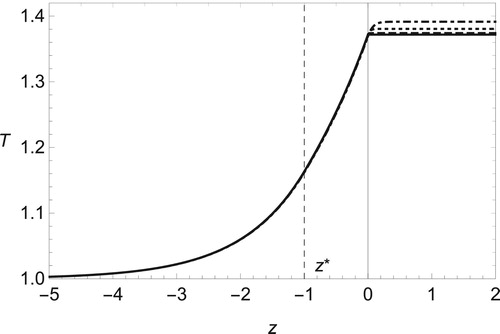
Figure 10. The same as Figure 9 but for fixed value of Mach number Ma = 0.3 with $Pr=1/4$ (solid line), 2/4 (dashed), 3/4 (dotted) and 1 (dot-dashed).

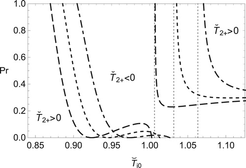
At last, in order to clarify the compressibility effect, we present the boundary determining the sign of ${\check{T}}_{2+}$ with respect to $T_i$, q and Pr. In Figures 11 and 12, the influence of $T_i$ and q on that boundary is shown. For a fixed value of ${\check{T}}_{i2}={\check{T}}_{i2ad}$, Figure 11 shows that the positive values of ${\check{T}}_{2+}$ are achieved easily by small values of q for some finite positive deviation of ${\check{T}}_{i0}$ from ${\check{T}}_{i0ad}$. This is feasible for small values of $Q_c$. Although there is a possibility of ${\check{T}}_{2+}>0$ for values of ${\check{T}}_{i0}$ sufficiently less than ${\check{T}}_{i0ad}$, it might be difficult because the demanded extent of deviation is large. On the other hand, Figure 12 shows the influence of ${\check{T}}_{i2}$ for a fixed value of ${\check{T}}_{i0}={\check{T}}_{i0ad}$. We find that the positive deviation of ${\check{T}}_{i2}$ from its adiabatic value leads to positive values of ${\check{T}}_{2+}$. From Figures 11 and 12, we also notice that large values of $Q_c$ make it difficult to obtain ${\check{T}}_{2+}>0$ for small deviations of ignition temperature from its adiabatic value. Figure 13 shows how the sign of ${\check{T}}_{2+}$ is influenced by the viscosity in some range of ignition temperature. The decrease of temperature, or ${\check{T}}_{2+}<0$, is achieved mostly in the case of ${\check{T}}_{i0}<{\check{T}}_{i0ad}$. For ${\check{T}}_{i0}>{\check{T}}_{i0ad}$, values of Prandtl number need to be small in order to obtain ${\check{T}}_{2+}<0$ for small heat release. The positive values of ${\check{T}}_{2+}$ is given by values of ${\check{T}}_{i0}$ sufficiently less than ${\check{T}}_{i0ad}$ or by small values of heat release for moderate values of Pr. If the Prandtl number and heat release are small enough, ${\check{T}}_{2+}>0$ may be obtained for small negative deviation of ${\check{T}}_{i0}$ from ${\check{T}}_{i0ad}$.

Figure 11. Boundary for sign of ${\check{T}}_{2+}$ with respect to ${\check{T}}_{i0}$ and q for fixed parameters ${\check{T}}_{i2}={\check{T}}_{i2ad}$, $\gamma =1.4$ and $Pr=3/4$. Value of ${\check{T}}_{2+}$ is negative in the domain surrounded by two curves and positive in the other two domains with Q = 0.5 (dashed line), 1 (dotted) and 2 (dot-dashed). As a reference, ${\check{T}}_{i0ad}$ is also plotted by solid lines for each value of Q.

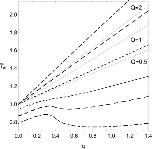
Figure 12. Boundary for sign of ${\check{T}}_{2+}$ with respect to ${\check{T}}_{i2}$ and q for fixed parameters ${\check{T}}_{i0}={\check{T}}_{i0ad}$, $\gamma =1.4$ and $Pr=3/4$. Value of ${\check{T}}_{2+}$ is negative (positive) below (over) each curve with Q = 0.5 (dashed line), 1 (dotted) and 2 (dot-dashed). As a reference, ${\check{T}}_{i2ad}$ is also plotted by solid lines for each value of Q.

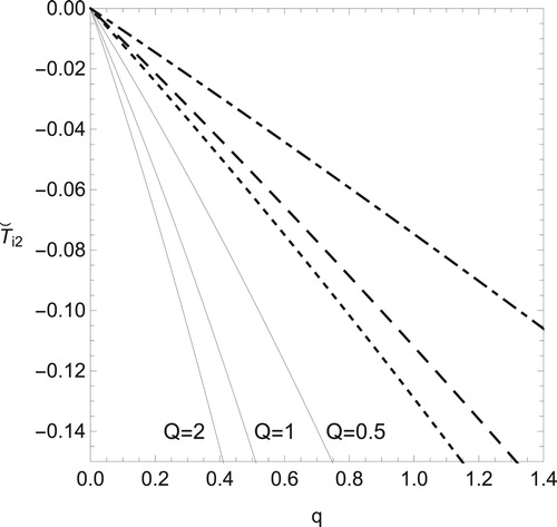
Figure 13. Boundary for sign of ${\check{T}}_{2+}$ with respect to ${\check{T}}_{i0}$ and Pr for fixed parameters ${\check{T}}_{i2}={\check{T}}_{i2ad}$, $\gamma =1.4$ and $Q_c=1$. Value of ${\check{T}}_{2+}$ is negative in the domain surrounded by two curves and positive in the other two domains with q = 0.01 (dashed line), 0.05 (dotted) and 0.1 (dot-dashed). Vertical dashed lines denote values of ${\check{T}}_{i0ad}$, which are asymptotes of each curve for corresponding values of q.

6. Conclusions

We have employed the method of matched asymptotic expansions with respect to small squared Mach numbers, ${Ma}^2\ll 1$, to study the non-adiabatic feature of a premixed flame front. By considering the additional region of $O\left({Ma}^2\right)$ thickness behind a flame front, we have derived the non-zero condition of temperature gradient at the burned-side edge of the front. By this condition, the non-adiabatic behaviour of temperature is realised depending on the values of ignition temperature. The value of ignition temperature is able to be determined for the adiabatic case. The non-adiabatic case is investigated by setting the value of ignition temperature less or larger than adiabatic one. If the ignition temperature is less than its adiabatic one, the decrease of temperature on the burned side due to gas compression is observed. On the other hand, the ignition temperature larger than its adiabatic one brings the monotonic increase of temperature with its maximum value beyond the adiabatic one. Although we do not have the comparable experimental data for temperature distribution in spatial field, our results may be compared qualitatively with those obtained numerically in previous works without contradiction. The boundary, which determines whether the temperature is increased or decreased due to the compressibility effect, is calculated with respect to the ignition temperature, the heat release and the Prandtl number. The effect of reaction rate on this boundary is also examined.

In the analysis of compression zone, we find that inner solutions are obtained by use of the Lambert W function. It is clear that the pressure and dissipation terms in the heat-conduction equation bring the non-adiabatic profile. This mechanism of temperature decrease is different from the conductive or volumetric heat loss which is realised by the phenomenological term describing Newton's law of cooling. Our result is due to pure compressibility effect.

The main assumption of our study is the strong ignition temperature approximation supposed by [60–62]. Thanks to this, it is possible to obtain exact solutions in the outer region, composed of the reaction and preheat zones. However, in this case, the cold boundary difficulty problem appears as a result of the constancy of reaction rate. This issue must be resolved, for example, by using the method of large activation energy asymptotics. This problem will be treated in the future work by considering the reaction rate in the form of Arrhenius type, which has an explicit temperature dependence [64,65].

Disclosure statement

No potential conflict of interest was reported by the author(s).

Appendix 1

Calculation of inner solutions ${\check{v}}_2$ and ${\check{p}}_2$

In this appendix, we calculate the inner solutions ${\check{v}}_2$ and ${\check{p}}_2$ in the compression zone. For the sake of the simplification of calculation below, we collect $O\left({Ma}^2\right)$ terms of (6(6) $\begin{array}{rl}P& =RT,\end{array}$(6) ) and (9(9) $M=RV\equiv 1.$(9) ), with (13(13a) $\begin{array}{rl}R& ={\check{\rho }}_0+{Ma}^2{\check{\rho }}_2,V={\check{v}}_0+{Ma}^2{\check{v}}_2,P={\check{p}}_0+{Ma}^2{\check{p}}_2,\end{array}$(13a) ) substituted. (A1) ${\check{p}}_2={\check{\rho }}_2{\check{\theta }}_0+{\check{\rho }}_0{\check{\theta }}_2,0={\check{\rho }}_2{\check{v}}_0+{\check{\rho }}_0{\check{v}}_2.$(A1) By use of (17(17) ${\check{p}}_0={\check{\rho }}_0{\check{\theta }}_0,1={\check{\rho }}_0{\check{v}}_0.$(17) ), two equations of (A1(A1) ${\check{p}}_2={\check{\rho }}_2{\check{\theta }}_0+{\check{\rho }}_0{\check{\theta }}_2,0={\check{\rho }}_2{\check{v}}_0+{\check{\rho }}_0{\check{v}}_2.$(A1) ) are combined into (A2) ${\check{v}}_2=\frac{{\check{\theta }}_2}{{\check{p}}_0}-\frac{{\check{v}}_0}{{\check{p}}_0}{\check{p}}_2.$(A2) Taking $\xi =0$ and $\xi \to +\mathrm{\infty }$ in (A2(A2) ${\check{v}}_2=\frac{{\check{\theta }}_2}{{\check{p}}_0}-\frac{{\check{v}}_0}{{\check{p}}_0}{\check{p}}_2.$(A2) ) and using (73(73) $\begin{array}{rl}{\check{V}}_0& =\left\{\begin{array}{ll}{\check{T}}_0& (z\le 0)\\ {\check{V}}_{0+}& (z>0)\end{array}\right.,\end{array}$(73) ) and (75(75) $\begin{array}{rl}{\check{P}}_0& =\left\{\begin{array}{ll}1& (z\le 0)\\ \sigma /{\check{V}}_{0+}& (z>0)\end{array}\right.,\end{array}$(75) ), we find (A3) ${\check{V}}_{2-}={\check{T}}_{2-}-\sigma {\check{P}}_{2-},{\check{V}}_{2+}=\frac{{\check{V}}_{0+}}{\sigma }{\check{T}}_{2+}-\frac{{\check{V}}_{0+}^2}{\sigma }{\check{P}}_{2+},$(A3) where ${\check{T}}_{2+}$, ${\check{V}}_{0+}$ and ${\check{T}}_{2-}$ are already obtained in (48(48) $\begin{array}{rl}{\check{T}}_{2+}& ={\check{T}}_{2-}+\frac{1}{2}\frac{\gamma -1}{\gamma }\nu {\check{V}}_{0+}^2\left({\left(\frac{{\check{V}}_{0-}}{{\check{V}}_{0+}}\right)}^2-1\right).\end{array}$(48) ), (83(83) ${\check{V}}_{0+}=\frac{(\gamma -1){\sigma }^2}{(2\gamma -1)\sigma -\gamma (1+q)}.$(83) ) and (86(86) $\begin{array}{rl}{\check{T}}_{2-}& ={\check{T}}_{i2}{\mathrm{e}}^{-z^{\ast }}+({\check{T}}_{i0}-1)\left(({\check{T}}_{i0}-1)\left(B+\frac{\gamma -1}{2}\right)+B\right)(1-{\mathrm{e}}^{-z^{\ast }})\\ & +q{Q}_c\left(q{Q}_{c}B-(\gamma -1)\left(\sigma -A{\mathrm{e}}^{-z^{\ast }}\right)\right)(1-z^{\ast }-{\mathrm{e}}^{-z^{\ast }})\\ & -(\gamma -1)q^2{Q}_c^2\left(z^{\ast }\left(1-{\mathrm{e}}^{-z^{\ast }}\right)-\frac{{z^{\ast }}^2}{2}\right)-A^2\left(B+\frac{\gamma -1}{2}\right)(1-{\mathrm{e}}^{-z^{\ast }}{)}^2\\ & -A\left(\frac{\gamma -1}{\gamma }\nu q{Q}_c+B(\sigma -A{\mathrm{e}}^{-z^{\ast }})\right)\left(1-(1+z^{\ast }){\mathrm{e}}^{-z^{\ast }}\right)\\ & -ABq{Q}_c\left(z^{\ast }(1-{\mathrm{e}}^{-z^{\ast }})-\frac{{z^{\ast }}^2}{2}{\mathrm{e}}^{-z^{\ast }}\right).\end{array}$(86) ), and ${\check{P}}_{2-}$ is calculated by taking z = 0 in (76(76) $\begin{array}{rl}{\check{P}}_2& =\left\{\begin{array}{ll}(\nu -\gamma )({\check{T}}_{i0}-1){\mathrm{e}}^{z-z^{\ast }}& (z\le z^{\ast })\\ (\nu -\gamma )\left\{q{Q}_c+A{\mathrm{e}}^{z-z^{\ast }}\right\}-\gamma q{Q}_c(z-z^{\ast })& (z^{\ast }<z\le 0)\\ {\check{P}}_{2+}& (z>0)\end{array}\right..\end{array}$(76) ) as (A4) ${\check{P}}_{2-}=(\nu -\gamma )\left(q{Q}_c+A{\mathrm{e}}^{-z^{\ast }}\right)+\gamma q{Q}_c{z}^{\ast }.$(A4) The value of ${\check{P}}_{2+}$ is computed in Appendix 2.

Now, we calculate the solution ${\check{v}}_2$. Substituting (13a(13a) $\begin{array}{rl}R& ={\check{\rho }}_0+{Ma}^2{\check{\rho }}_2,V={\check{v}}_0+{Ma}^2{\check{v}}_2,P={\check{p}}_0+{Ma}^2{\check{p}}_2,\end{array}$(13a) ) into (3(3) $\begin{array}{rl}M\frac{\mathrm{d}V}{\mathrm{d}z}& =-\frac{1}{\gamma {Ma}^2}\frac{\mathrm{d}P}{\mathrm{d}z}+\frac{4}{3}Pr\frac{{\mathrm{d}}^{2}V}{\mathrm{d}{z}^2},\end{array}$(3) ), the $O\left({Ma}^2\right)$ terms are collected as (A5) $\gamma \frac{\mathrm{d}{\check{v}}_0}{\mathrm{d}\xi }=-\frac{\mathrm{d}{\check{p}}_2}{\mathrm{d}\xi }+\nu \frac{{\mathrm{d}}^2{\check{v}}_2}{\mathrm{d}{\xi }^2}.$(A5) The integration of (A5(A5) $\gamma \frac{\mathrm{d}{\check{v}}_0}{\mathrm{d}\xi }=-\frac{\mathrm{d}{\check{p}}_2}{\mathrm{d}\xi }+\nu \frac{{\mathrm{d}}^2{\check{v}}_2}{\mathrm{d}{\xi }^2}.$(A5) ) leads to (A6) ${\check{p}}_2=\nu \frac{\mathrm{d}{\check{v}}_2}{\mathrm{d}\xi }-\gamma {\check{v}}_0+{\check{p}}_{2c},$(A6) where ${\check{p}}_{2c}$ is an integral constant. Taking the limit $\xi \to +\mathrm{\infty }$ in (A6(A6) ${\check{p}}_2=\nu \frac{\mathrm{d}{\check{v}}_2}{\mathrm{d}\xi }-\gamma {\check{v}}_0+{\check{p}}_{2c},$(A6) ), by use of (14a(14a) $\begin{array}{rl}{\check{\phi }}_0{|}_{\xi \to +\mathrm{\infty }}& ={\check{\mathrm{\Phi }}}_0{|}_{z\to 0+},{\check{\phi }}_2{|}_{\xi \to +\mathrm{\infty }}={\check{\mathrm{\Phi }}}_2{|}_{z\to 0+}+\xi \frac{\mathrm{d}{\check{\mathrm{\Phi }}}_0}{\mathrm{d}z}{|}_{z\to 0+},\end{array}$(14a) ) and (14b(14b) $\begin{array}{rl}\frac{\mathrm{d}{\check{\phi }}_0}{\mathrm{d}\xi }{|}_{\xi \to +\mathrm{\infty }}& =0,\frac{\mathrm{d}{\check{\phi }}_2}{\mathrm{d}\xi }{|}_{\xi \to +\mathrm{\infty }}=\frac{\mathrm{d}{\check{\mathrm{\Phi }}}_0}{\mathrm{d}z}{|}_{z\to 0+}.\end{array}$(14b) ), ${\check{p}}_{2c}$ is determined as (A7) ${\check{p}}_{2c}={\check{P}}_{2+}+\gamma {\check{V}}_{0+}.$(A7) Equation (A2(A2) ${\check{v}}_2=\frac{{\check{\theta }}_2}{{\check{p}}_0}-\frac{{\check{v}}_0}{{\check{p}}_0}{\check{p}}_2.$(A2) ) helps us to rewrite (A6(A6) ${\check{p}}_2=\nu \frac{\mathrm{d}{\check{v}}_2}{\mathrm{d}\xi }-\gamma {\check{v}}_0+{\check{p}}_{2c},$(A6) ) into the following differential equation for ${\check{v}}_2$. (A8) $\nu \frac{\mathrm{d}{\check{v}}_2}{\mathrm{d}\xi }+\frac{{\check{p}}_0}{{\check{v}}_0}{\check{v}}_2=\frac{{\check{\theta }}_2}{{\check{v}}_0}+\gamma {\check{v}}_0-{\check{p}}_{2c}.$(A8) We note that ${\check{v}}_0$, ${\check{p}}_0$ and ${\check{\theta }}_2$ are already obtained in (33(33) ${\check{v}}_0={\check{V}}_{0+}\left(1+W\right).$(33) ), (34(34) ${\check{p}}_0=\frac{{\check{P}}_{0+}}{1+W},$(34) ) and (40(40) ${\check{\theta }}_2=C^{\prime }+\frac{\mathrm{d}{\check{T}}_0}{\mathrm{d}z}{|}_{+}\xi -\frac{\gamma -1}{\gamma }\nu {\check{V}}_{0+}^{2}W\left(1+\frac{W}{2}\right).$(40) ). The solution of (A8(A8) $\nu \frac{\mathrm{d}{\check{v}}_2}{\mathrm{d}\xi }+\frac{{\check{p}}_0}{{\check{v}}_0}{\check{v}}_2=\frac{{\check{\theta }}_2}{{\check{v}}_0}+\gamma {\check{v}}_0-{\check{p}}_{2c}.$(A8) ) is calculated as (A9) $\begin{array}{rl}{\check{v}}_2& =\frac{1}{{\check{P}}_{0+}}\frac{W}{1+W}\left\{{\check{v}}_{2c}+({\check{T}}_{2+}-{\check{P}}_{2+}{\check{V}}_{0+})\left(\frac{1}{W}-\ln |W|\right)\right.\\ & \left.-\frac{1+\gamma -B}{4}{\check{V}}_{0+}^{2}W(2+W)+\frac{{\check{P}}_{0+}}{\nu }\left({\check{V}}_{0+}\right(1-B)-{\check{P}}_{2+})\xi \right\},\end{array}$(A9) where ${\check{v}}_{2c}$ is an integral constant. Taking $\xi =0$ in (A9(A9) $\begin{array}{rl}{\check{v}}_2& =\frac{1}{{\check{P}}_{0+}}\frac{W}{1+W}\left\{{\check{v}}_{2c}+({\check{T}}_{2+}-{\check{P}}_{2+}{\check{V}}_{0+})\left(\frac{1}{W}-\ln |W|\right)\right.\\ & \left.-\frac{1+\gamma -B}{4}{\check{V}}_{0+}^{2}W(2+W)+\frac{{\check{P}}_{0+}}{\nu }\left({\check{V}}_{0+}\right(1-B)-{\check{P}}_{2+})\xi \right\},\end{array}$(A9) ), the integral constant ${\check{v}}_{2c}$ is determined as ${\check{v}}_{2c}=\frac{1+\alpha }{\alpha }{\check{P}}_{0+}{\check{V}}_{2-}-({\check{T}}_{2+}-{\check{P}}_{2+}{\check{V}}_{0+})\left(\frac{1}{\alpha }-\ln |\alpha |\right)+\frac{1+\gamma -B}{4}{\check{V}}_{0+}^2\alpha (2+\alpha ),$where α is defined by (A10) $\alpha =\frac{{\check{V}}_{0-}}{{\check{V}}_{0+}}-1.$(A10) By the use of (A9(A9) $\begin{array}{rl}{\check{v}}_2& =\frac{1}{{\check{P}}_{0+}}\frac{W}{1+W}\left\{{\check{v}}_{2c}+({\check{T}}_{2+}-{\check{P}}_{2+}{\check{V}}_{0+})\left(\frac{1}{W}-\ln |W|\right)\right.\\ & \left.-\frac{1+\gamma -B}{4}{\check{V}}_{0+}^{2}W(2+W)+\frac{{\check{P}}_{0+}}{\nu }\left({\check{V}}_{0+}\right(1-B)-{\check{P}}_{2+})\xi \right\},\end{array}$(A9) ), ${\check{p}}_2$ is calculated from (A6(A6) ${\check{p}}_2=\nu \frac{\mathrm{d}{\check{v}}_2}{\mathrm{d}\xi }-\gamma {\check{v}}_0+{\check{p}}_{2c},$(A6) ) as follows. (A11) $\begin{array}{rl}{\check{p}}_2& =\frac{1}{{\check{V}}_{0+}}\frac{W}{(1+W{)}^3}\left\{-{\check{v}}_{2c}+({\check{T}}_{2+}-{\check{P}}_{2+}{\check{V}}_{0+})(2+W+\ln |W|)\right.\\ & +\frac{1+\gamma -B}{4}{\check{V}}_{0+}^{2}W(4+5W+2W^2)\\ & \left.+\left({\check{V}}_{0+}\right(1-B)-{\check{P}}_{2+})\left({\check{V}}_{0+}(1+W{)}^2-\frac{{\check{P}}_{0+}}{\nu }\xi \right)\right\}-\gamma {\check{V}}_{0+}W+{\check{P}}_{2+}.\end{array}$(A11) We note that the sign in removing the absolute symbol of $|W|$, included in (A9(A9) $\begin{array}{rl}{\check{v}}_2& =\frac{1}{{\check{P}}_{0+}}\frac{W}{1+W}\left\{{\check{v}}_{2c}+({\check{T}}_{2+}-{\check{P}}_{2+}{\check{V}}_{0+})\left(\frac{1}{W}-\ln |W|\right)\right.\\ & \left.-\frac{1+\gamma -B}{4}{\check{V}}_{0+}^{2}W(2+W)+\frac{{\check{P}}_{0+}}{\nu }\left({\check{V}}_{0+}\right(1-B)-{\check{P}}_{2+})\xi \right\},\end{array}$(A9) ) and (A11(A11) $\begin{array}{rl}{\check{p}}_2& =\frac{1}{{\check{V}}_{0+}}\frac{W}{(1+W{)}^3}\left\{-{\check{v}}_{2c}+({\check{T}}_{2+}-{\check{P}}_{2+}{\check{V}}_{0+})(2+W+\ln |W|)\right.\\ & +\frac{1+\gamma -B}{4}{\check{V}}_{0+}^{2}W(4+5W+2W^2)\\ & \left.+\left({\check{V}}_{0+}\right(1-B)-{\check{P}}_{2+})\left({\check{V}}_{0+}(1+W{)}^2-\frac{{\check{P}}_{0+}}{\nu }\xi \right)\right\}-\gamma {\check{V}}_{0+}W+{\check{P}}_{2+}.\end{array}$(A11) ), depends on the value of ignition temperature $T_i$. For example, if ${\check{T}}_{i0}<{\check{T}}_{i0ad}$, we find $\sigma <1+q$ from (66(66) $\begin{array}{rl}\sigma & =1+q{Q}_c(1-z^{\ast })+A{\mathrm{e}}^{-z^{\ast }},\end{array}$(66) ) and (89a(89a) $\begin{array}{rl}{\check{T}}_{i0ad}& =1+q{Q}_c(1-{\mathrm{e}}^{z^{\ast }}),\end{array}$(89a) ). Then, (83(83) ${\check{V}}_{0+}=\frac{(\gamma -1){\sigma }^2}{(2\gamma -1)\sigma -\gamma (1+q)}.$(83) ) leads to ${\check{V}}_{0+}>\sigma (={\check{V}}_{0-})$. In this case, we get W<0 due to (30(30) $\left(\frac{{\check{v}}_0}{{\check{V}}_{0+}}-1\right)\exp \left(\frac{{\check{v}}_0}{{\check{V}}_{0+}}-1\right)=\left(\frac{{\check{V}}_{0-}}{{\check{V}}_{0+}}-1\right)\exp \left(-\frac{1}{\nu }\frac{{\check{P}}_{0+}}{{\check{V}}_{0+}}\xi +\frac{{\check{V}}_{0-}}{{\check{V}}_{0+}}-1\right).$(30) ) and (33(33) ${\check{v}}_0={\check{V}}_{0+}\left(1+W\right).$(33) ). On the other hand, we obtain W>0 for ${\check{T}}_{i0}>{\check{T}}_{i0ad}$.

Appendix 2

Computation of ${\check{P}}_{2+}$

To determine the value of ${\check{P}}_{2+}$, we consider $O\left({Ma}^4\right)$ term of asymptotic expansions for the temperature, ${\check{\theta }}_4$, as an extension of the first equation of (13b(13b) $\begin{array}{rl}T& ={\check{\theta }}_0+{Ma}^2{\check{\theta }}_2,Y={\check{c}}_0+{Ma}^2{\check{c}}_2.\end{array}$(13b) ). Then, collecting $O\left({Ma}^4\right)$ terms in (4(4) $\begin{array}{rl}M\frac{\mathrm{d}T}{\mathrm{d}z}& =\frac{{\mathrm{d}}^{2}T}{\mathrm{d}{z}^2}+\frac{\gamma -1}{\gamma }V\frac{\mathrm{d}P}{\mathrm{d}z}+\frac{4}{3}(\gamma -1)Pr{Ma}^2{\left(\frac{\mathrm{d}V}{\mathrm{d}z}\right)}^2+qQ,\end{array}$(4) ), we obtain the following equation in the compression zone. (A12) $\frac{\mathrm{d}{\check{\theta }}_2}{\mathrm{d}\xi }=\frac{{\mathrm{d}}^2{\check{\theta }}_4}{\mathrm{d}{\xi }^2}+\frac{\gamma -1}{\gamma }\left({\check{v}}_2\frac{\mathrm{d}{\check{p}}_0}{\mathrm{d}\xi }+{\check{v}}_0\frac{\mathrm{d}{\check{p}}_2}{\mathrm{d}\xi }+2\nu \frac{\mathrm{d}{\check{v}}_0}{\mathrm{d}\xi }\frac{\mathrm{d}{\check{v}}_2}{\mathrm{d}\xi }\right).$(A12) By integrating (A12(A12) $\frac{\mathrm{d}{\check{\theta }}_2}{\mathrm{d}\xi }=\frac{{\mathrm{d}}^2{\check{\theta }}_4}{\mathrm{d}{\xi }^2}+\frac{\gamma -1}{\gamma }\left({\check{v}}_2\frac{\mathrm{d}{\check{p}}_0}{\mathrm{d}\xi }+{\check{v}}_0\frac{\mathrm{d}{\check{p}}_2}{\mathrm{d}\xi }+2\nu \frac{\mathrm{d}{\check{v}}_0}{\mathrm{d}\xi }\frac{\mathrm{d}{\check{v}}_2}{\mathrm{d}\xi }\right).$(A12) ) from $\xi =0$ to $+\mathrm{\infty }$, we gain the equation to compute the value of ${\check{P}}_{2+}$, by use of (14a(14a) $\begin{array}{rl}{\check{\phi }}_0{|}_{\xi \to +\mathrm{\infty }}& ={\check{\mathrm{\Phi }}}_0{|}_{z\to 0+},{\check{\phi }}_2{|}_{\xi \to +\mathrm{\infty }}={\check{\mathrm{\Phi }}}_2{|}_{z\to 0+}+\xi \frac{\mathrm{d}{\check{\mathrm{\Phi }}}_0}{\mathrm{d}z}{|}_{z\to 0+},\end{array}$(14a) ) and (15(15) ${\check{\phi }}_0{|}_{\xi =0}={\check{\mathrm{\Phi }}}_0{|}_{z=0}={\check{\mathrm{\Phi }}}_0{|}_{z\to 0-},{\check{\phi }}_2{|}_{\xi =0}={\check{\mathrm{\Phi }}}_2{|}_{z=0}={\check{\mathrm{\Phi }}}_2{|}_{z\to 0-}.$(15) ), as (A13) ${\check{T}}_{2+}-{\check{T}}_{2-}=\frac{\mathrm{d}{\check{T}}_2}{\mathrm{d}z}{|}_{+}-\frac{\mathrm{d}{\check{T}}_2}{\mathrm{d}z}{|}_{-}+\frac{\gamma -1}{\gamma }{\int }_0^{+\mathrm{\infty }}\left({\check{v}}_2\frac{\mathrm{d}{\check{p}}_0}{\mathrm{d}\xi }+{\check{v}}_0\frac{\mathrm{d}{\check{p}}_2}{\mathrm{d}\xi }+2\nu \frac{\mathrm{d}{\check{v}}_0}{\mathrm{d}\xi }\frac{\mathrm{d}{\check{v}}_2}{\mathrm{d}\xi }\right)\mathrm{d}\xi ,$(A13) where we have also employed the following conditions, which are obtained as an extension of (14b(14b) $\begin{array}{rl}\frac{\mathrm{d}{\check{\phi }}_0}{\mathrm{d}\xi }{|}_{\xi \to +\mathrm{\infty }}& =0,\frac{\mathrm{d}{\check{\phi }}_2}{\mathrm{d}\xi }{|}_{\xi \to +\mathrm{\infty }}=\frac{\mathrm{d}{\check{\mathrm{\Phi }}}_0}{\mathrm{d}z}{|}_{z\to 0+}.\end{array}$(14b) ) and (79(79) $\begin{array}{rl}\frac{\mathrm{d}{\check{\theta }}_2}{\mathrm{d}\xi }{|}_{\xi =0}& =\frac{\mathrm{d}{\check{T}}_0}{\mathrm{d}z}{|}_{z=0},0=\frac{\mathrm{d}{\check{c}}_2}{\mathrm{d}\xi }{|}_{\xi =0}=\frac{\mathrm{d}{\check{Y}}_0}{\mathrm{d}z}{|}_{z=0}.\end{array}$(79) ) to higher order, $O\left({Ma}^4\right)$. $\frac{\mathrm{d}{\check{\theta }}_4}{\mathrm{d}\xi }{|}_{\xi \to +\mathrm{\infty }}=\frac{\mathrm{d}{\check{T}}_2}{\mathrm{d}z}{|}_{+}+\xi \frac{{\mathrm{d}}^2{\check{T}}_0}{\mathrm{d}{z}^2}{|}_{+},\frac{\mathrm{d}{\check{\theta }}_4}{\mathrm{d}\xi }{|}_{\xi =0}=\frac{\mathrm{d}{\check{T}}_2}{\mathrm{d}z}{|}_{-}.$We remark that the terms proportional to ξ, which are created due to the matching conditions, are found to disappear because of the constancy of temperature on the burned side as given by (71(71) $\begin{array}{rl}{\check{T}}_0& =\left\{\begin{array}{ll}1+({\check{T}}_{i0}-1){\mathrm{e}}^{z-z^{\ast }}& (z\le z^{\ast })\\ \sigma +A({\mathrm{e}}^{z-z^{\ast }}-{\mathrm{e}}^{-z^{\ast }})+q{Q}_{c}z& (z^{\ast }<z\le 0)\\ \sigma & (z>0)\end{array}\right.,\end{array}$(71) ).

The unknown parameter ${\check{P}}_{2+}$ is included in the integral term in (A13(A13) ${\check{T}}_{2+}-{\check{T}}_{2-}=\frac{\mathrm{d}{\check{T}}_2}{\mathrm{d}z}{|}_{+}-\frac{\mathrm{d}{\check{T}}_2}{\mathrm{d}z}{|}_{-}+\frac{\gamma -1}{\gamma }{\int }_0^{+\mathrm{\infty }}\left({\check{v}}_2\frac{\mathrm{d}{\check{p}}_0}{\mathrm{d}\xi }+{\check{v}}_0\frac{\mathrm{d}{\check{p}}_2}{\mathrm{d}\xi }+2\nu \frac{\mathrm{d}{\check{v}}_0}{\mathrm{d}\xi }\frac{\mathrm{d}{\check{v}}_2}{\mathrm{d}\xi }\right)\mathrm{d}\xi ,$(A13) ) as indicated by solutions (A9(A9) $\begin{array}{rl}{\check{v}}_2& =\frac{1}{{\check{P}}_{0+}}\frac{W}{1+W}\left\{{\check{v}}_{2c}+({\check{T}}_{2+}-{\check{P}}_{2+}{\check{V}}_{0+})\left(\frac{1}{W}-\ln |W|\right)\right.\\ & \left.-\frac{1+\gamma -B}{4}{\check{V}}_{0+}^{2}W(2+W)+\frac{{\check{P}}_{0+}}{\nu }\left({\check{V}}_{0+}\right(1-B)-{\check{P}}_{2+})\xi \right\},\end{array}$(A9) ) and (A11(A11) $\begin{array}{rl}{\check{p}}_2& =\frac{1}{{\check{V}}_{0+}}\frac{W}{(1+W{)}^3}\left\{-{\check{v}}_{2c}+({\check{T}}_{2+}-{\check{P}}_{2+}{\check{V}}_{0+})(2+W+\ln |W|)\right.\\ & +\frac{1+\gamma -B}{4}{\check{V}}_{0+}^{2}W(4+5W+2W^2)\\ & \left.+\left({\check{V}}_{0+}\right(1-B)-{\check{P}}_{2+})\left({\check{V}}_{0+}(1+W{)}^2-\frac{{\check{P}}_{0+}}{\nu }\xi \right)\right\}-\gamma {\check{V}}_{0+}W+{\check{P}}_{2+}.\end{array}$(A11) ). The value of ${\check{P}}_{2+}$ is computed so that (A13(A13) ${\check{T}}_{2+}-{\check{T}}_{2-}=\frac{\mathrm{d}{\check{T}}_2}{\mathrm{d}z}{|}_{+}-\frac{\mathrm{d}{\check{T}}_2}{\mathrm{d}z}{|}_{-}+\frac{\gamma -1}{\gamma }{\int }_0^{+\mathrm{\infty }}\left({\check{v}}_2\frac{\mathrm{d}{\check{p}}_0}{\mathrm{d}\xi }+{\check{v}}_0\frac{\mathrm{d}{\check{p}}_2}{\mathrm{d}\xi }+2\nu \frac{\mathrm{d}{\check{v}}_0}{\mathrm{d}\xi }\frac{\mathrm{d}{\check{v}}_2}{\mathrm{d}\xi }\right)\mathrm{d}\xi ,$(A13) ) holds. The values of ${\check{P}}_{2+}$ for some fixed parameters are shown in Table A1. For sufficiently mall viscosity, the increase of deviations of ignition temperature from its adiabatic value leads to the increase of ${\check{P}}_{2+}$ for ${\check{T}}_i<{\check{T}}_{iad}$ and the decrease for ${\check{T}}_i>{\check{T}}_{iad}$. On the other hand, for some moderate values of Prandtl number, we find the opposite tendency.

Table A1. The values of ${\check{P}}_{2+}$ are computed from (A13(A13) ${\check{T}}_{2+}-{\check{T}}_{2-}=\frac{\mathrm{d}{\check{T}}_2}{\mathrm{d}z}{|}_{+}-\frac{\mathrm{d}{\check{T}}_2}{\mathrm{d}z}{|}_{-}+\frac{\gamma -1}{\gamma }{\int }_0^{+\mathrm{\infty }}\left({\check{v}}_2\frac{\mathrm{d}{\check{p}}_0}{\mathrm{d}\xi }+{\check{v}}_0\frac{\mathrm{d}{\check{p}}_2}{\mathrm{d}\xi }+2\nu \frac{\mathrm{d}{\check{v}}_0}{\mathrm{d}\xi }\frac{\mathrm{d}{\check{v}}_2}{\mathrm{d}\xi }\right)\mathrm{d}\xi ,$(A13) ) for several values of $d={\check{T}}_{i0}-{\check{T}}_{i0ad}$, which represent the deviations of ignition temperature from its adiabatic values and play the role of measurement of non-adiabaticity.

d	$-0.3$		$-0.15$		0		0.15		0.3
Pr	1/4	3/4	1/4	3/4	1/4	3/4	1/4	3/4	1/4	3/4
${\check{P}}_{2+}$	−5.07	−12.65	−7.2	−9.45	−8.4		−9.55	−8.09	−10.75	−8.1
${\check{T}}_{2+}$	−14.37	−28.2	−10.67	−15.03	−9.6		−9.29	−6.31	−9.28	−3.81
${\check{T}}_{2-}$	−8.12	−9.47	−8.85	−9.57	−9.6		−10.37	−9.57	−11.17	−9.47

Notes: Parameters are set as ${\check{T}}_{i2}={\check{T}}_{i2ad}$, q = 6, $Q_c=1$ and $\gamma =1.4$. In this case, adiabatic ignition temperature is calculated from (89a(89a) $\begin{array}{rl}{\check{T}}_{i0ad}& =1+q{Q}_c(1-{\mathrm{e}}^{z^{\ast }}),\end{array}$(89a) ) and (89b(89b) $\begin{array}{rl}{\check{T}}_{i2ad}& =({\check{T}}_{i0}-1)\left(({\check{T}}_{i0}-1)\left(B+\frac{\gamma -1}{2}\right)+B\right)-(\gamma -1)q^2{Q}_c^2{z}^{\ast }\\ & -q{Q}_c\left(q{Q}_{c}B-(\gamma -1)\left(\sigma -A{\mathrm{e}}^{-z^{\ast }}\right)\right)({\mathrm{e}}^{z^{\ast }}-1)-ABq{Q}_c{z}^{\ast }\left(1+\frac{z^{\ast }}{2}\right)\\ & -A^2(2B+\gamma -1)(1-{\mathrm{e}}^{-z^{\ast }})-A\left(\frac{\gamma -1}{\gamma }\nu q{Q}_c+B(\sigma -A{\mathrm{e}}^{-z^{\ast }})\right)z^{\ast }.\end{array}$(89b) ) as ${\check{T}}_{i0ad}\approx 4.79$ and ${\check{T}}_{i2ad}$ depends on ${\check{T}}_{i0}$ and Pr. The non-adiabatic feature of temperature is identified from ${\check{T}}_{2+}$ and ${\check{T}}_{2-}$.

The values of ${\check{T}}_{2+}$ and ${\check{T}}_{2-}$, which are given in (48(48) $\begin{array}{rl}{\check{T}}_{2+}& ={\check{T}}_{2-}+\frac{1}{2}\frac{\gamma -1}{\gamma }\nu {\check{V}}_{0+}^2\left({\left(\frac{{\check{V}}_{0-}}{{\check{V}}_{0+}}\right)}^2-1\right).\end{array}$(48) ) and (86(86) $\begin{array}{rl}{\check{T}}_{2-}& ={\check{T}}_{i2}{\mathrm{e}}^{-z^{\ast }}+({\check{T}}_{i0}-1)\left(({\check{T}}_{i0}-1)\left(B+\frac{\gamma -1}{2}\right)+B\right)(1-{\mathrm{e}}^{-z^{\ast }})\\ & +q{Q}_c\left(q{Q}_{c}B-(\gamma -1)\left(\sigma -A{\mathrm{e}}^{-z^{\ast }}\right)\right)(1-z^{\ast }-{\mathrm{e}}^{-z^{\ast }})\\ & -(\gamma -1)q^2{Q}_c^2\left(z^{\ast }\left(1-{\mathrm{e}}^{-z^{\ast }}\right)-\frac{{z^{\ast }}^2}{2}\right)-A^2\left(B+\frac{\gamma -1}{2}\right)(1-{\mathrm{e}}^{-z^{\ast }}{)}^2\\ & -A\left(\frac{\gamma -1}{\gamma }\nu q{Q}_c+B(\sigma -A{\mathrm{e}}^{-z^{\ast }})\right)\left(1-(1+z^{\ast }){\mathrm{e}}^{-z^{\ast }}\right)\\ & -ABq{Q}_c\left(z^{\ast }(1-{\mathrm{e}}^{-z^{\ast }})-\frac{{z^{\ast }}^2}{2}{\mathrm{e}}^{-z^{\ast }}\right).\end{array}$(86) ), are also listed in Table A1 to help understanding the effect of compressibility on the decrease of temperature due to the change of ignition temperature and viscosity. The temperature profiles are shown in Figures 3–10 in Section 5 for several cases of d = 0 (adiabatic case) and $d\ne 0$ (non-adiabatic cases).

References

- E. Mallard and H.L. Le-Chatelier, Thermal model for flame propagation, Ann. Mines 4 (1883), pp. 379.
- B. Lewis and G. von Elbe, Theory of flame propagation, Chem. Rev. 21 (1937), pp. 347–358. doi: 10.1021/cr60069a011
- G.I. Sivashinsky, On a distorted flame front as a hydrodynamic discontinuity, Acta Astronaut. 3 (1976), pp. 889–918. doi: 10.1016/0094-5765(76)90001-1
- B.J. Matkowsky and G.I. Sivashinsky, An asymptotic derivation of two models in flame theory associated with the constant density approximation, SIAM J. Appl. Math. 37 (1979), pp. 686–699. doi: 10.1137/0137051
- G.I. Sivashinsky, Structure of bunsen flames, J. Chem. Phys. 62 (1975), pp. 638–643. doi: 10.1063/1.430465
- W.B. Bush and F.E. Fendell, Asymptotic analysis of laminar flame propagation for general lewis numbers, Combust. Sci. Tech. 1 (1970), pp. 421–428. doi: 10.1080/00102206908952222
- R. Friedman and E. Burke, A theoretical model of a gaseous combustion wave governed by a first-order reaction, J. Chem. Phys. 21 (1953), pp. 710–714. doi: 10.1063/1.1698995
- T. von Kármán, The present status of the theory of laminar flame propagation, Sixth Symposium on Combustion, Reinhold, New York, 1957, pp. 1–11.
- G. Joulin and P. Vidal, Hydrodynamics and nonlinear instabilities, Cambridge University Press, Cambridge, 1998.
- G.I. Sivashinsky, Nonlinear analysis of hydrodynamic instability in laminar flames–I. Derivation of basic equations, Acta Astronaut. 4 (1977), pp. 1177–1206. doi: 10.1016/0094-5765(77)90096-0
- P. Clavin and F.A. Williams, Effects of molecular diffusion and of thermal expansion on the structure and dynamics of premixed flames in turbulent flows of large scale and low intensity, J. Fluid Mech.116 (1982), pp. 251–282. doi: 10.1017/S0022112082000457
- P. Pelce and P. Clavin, Influence of hydrodynamics and diffusion upon the stability limits of laminar premixed flames, J. Fluid Mech. 124 (1982), pp. 219–237. doi: 10.1017/S002211208200247X
- M. Matalon and B.J. Matkowsky, Flames as gasdynamic discontinuities, J. Fluid Mech. 124 (1982), pp. 239–259. doi: 10.1017/S0022112082002481
- M. Matalon, C. Cui, and J.K. Bechtold, Hydrodynamic theory of premixed flames: effects of stoichiometry, variable transport coefficients and arbitrary reaction orders, J. Fluid Mech. 487 (2003), pp. 179–210. doi: 10.1017/S0022112003004683
- I. Glassman and R.A. Yetter, Combustion. 4th ed.Academic Press, Burlington, 2008.
- Y.B. Zel'dovich and D.A. Frank-Kamenetskii, Theory of thermal flame propagation, Zhu. Fiz. Khim.12 (1938), pp. 100–105.
- Y.B. Zel'dovich and D.A. Frank-Kamenetskii, A theory of thermal propagation of flame, Acta Phys. URRS 9 (1938), pp. 341–350.
- C.K. Law, Combustion physics, Cambridge University Press, Cambridge, 2006.
- A. Liñán, The asymptotic structure of counterflow diffusion flames for large activation energies, Acta. Astronaut. 1 (1974), pp. 1007–1039. doi: 10.1016/0094-5765(74)90066-6
- P.L. Simon, S. Kalliadasis, J.H. Merkin, and S.K. Scott, Quenching of flame propagation with heat loss, J. Math. Chem. 31 (2002), pp. 313–332. doi: 10.1023/A:1020840222396
- D.B. Spalding, A theory of inflammability limits and flame-quenching, Proc. Roy. Soc. (Lond.) 240 (1957), pp. 83–100.
- J. Buckmaster, The quenching of two-dimensional premixed flames, Acta Astronaut.6 (1979), pp. 741–769. doi: 10.1016/0094-5765(79)90031-6
- S. Kadowaki, The effects of heat loss on the burning velocity of cellular premixed flames generated by hydrodynamic and diffusive-thermal instabilities, Combust. Flame 143 (2005), pp. 174–182. doi: 10.1016/j.combustflame.2005.05.012
- S. Kadowaki, H. Takahashi, and H. Kobayashi, The effects of radiation on the dynamic behavior of cellular premixed flames generated by intrinsic instability, Proc. Combust. Inst. 33 (2011), pp. 1153–1162. doi: 10.1016/j.proci.2010.06.069
- F.A. Williams, Combustion theory: the fundamental theory of chemically reacting flow systems. 2nd ed.Addison-Wesley, Menlo Park, 1985.
- L. Kagan and G.I. Sivashinsky, Deflagration-to-detonation transition in narrow channels: Hydraulic resistance vs. flame folding, 25th ICDERS Leeds, UK (2015).
- V.N. Kurdyumov and M. Matalon, Critical conditions for flame acceleration in long adiabatic channels closed at their ignition end, Proc. Combust. Inst. 36 (2017), pp. 1549–1557. doi: 10.1016/j.proci.2016.06.024
- V. Bychkov, M. Modestov, and M. Marklund, The Darrieus-Landau instability in fast deflagration and laser ablation, Phys. Plasmas 1(5) (2008), pp. 032702.
- M. Modestov, V. Bychkov, D. Valiev, and M. Marklund, Growth rate and the cutoff wavelength of the Darrieus-Landau instability in laser ablation. Phys. Rev. E 8(0) (2009046403.
- W. Hillebrandt and J.C. Niemeyer, Type Ia supernova explosion models. Annu. Rev. Astron. Astrophys. 38 (2000), pp. 191–230. doi: 10.1146/annurev.astro.38.1.191
- V. Bychkov, M. Modestov, V. Akkerman, and L.E. Eriksson, The Rayleigh–Taylor instability in inertial fusion, astrophysical plasma and flames, Plasma Phys. Control. Fusion 49 (2007), pp. B513–B520. doi: 10.1088/0741-3335/49/12B/S49
- I. Brailovsky and G.I. Sivashinsky, Hydraulic resistance as a mechanism for deflagration-to-detonation transition, Combust. Flame 122 (2000), pp. 492–499. doi: 10.1016/S0010-2180(00)00157-7
- B. Demirgok, O. Ugarte, D. Valiev, and V. Akkerman, Effect of thermal expansion on flame propagation in channels with nonslip walls, Proc. Combust. Inst. 35 (2015), pp. 929–936. doi: 10.1016/j.proci.2014.07.031
- V.N. Kurdyumov and M. Matalon, Effects of gas compressibility on the dynamics of premixed flames in long narrow adiabatic channels, Combust. Theory Model. 20:62016), pp. 1046–1067. doi: 10.1080/13647830.2016.1245444
- G. Darrieus, unpublished works presented at la technique moderne (1938).
- L.D. Landau, On the theory of slow combustion, Acta Phys. (USSR) 19 (1944
- V. Bychkov, V. Akkerman, D. Valiev, and C.K. Law, Role of compressibility in moderating flame acceleration in tubes, Phys. Rev. E 8(1) (2010), pp. 026309. doi: 10.1103/PhysRevE.95.013111
- D.M. Valiev, V. Akkerman, M. Kuznetsov, L.E. Eriksson, C.K. Law, and V. Bychkov, Influence of gas compression on flame acceleration in the early stage of burning in tubes, Combust. Flame 160 (2013), pp. 97–111. doi: 10.1016/j.combustflame.2012.09.002
- S. Demir, A.R. Calavay, and V. Akkerman, Influence of gas compressibility on a burning accident in a mining passage, Combust. Theory Model. 22 (2018), pp. 338–358. doi: 10.1080/13647830.2017.1403654
- J.C. Wheeler and R.P. Harkness, Type I supernovae, Rep. Prog. Phys. 53 (1990), pp. 1467–1557. doi: 10.1088/0034-4885/53/12/001
- F.K. Röpke and S.A. Sim, Models for type Ia supernovae and related astrophysical transients. Space Sci. Rev. 21(4) (2018), p. 72. doi: 10.1007/s11214-018-0503-8
- J.R. Boisseau, J.C. Wheeler, E.S. Oran, and A.M. Khokhlov, The multidimensional structure of detonations in type Ia supernovae. Astrophys. J. 471 (1996), pp. L99–L102. doi: 10.1086/310338
- F. Hoyle and W.A. Fowler, Nucleosynthesis in supernovae, Astrophys. J. 132 (1960), pp. 565–590. doi: 10.1086/146963
- S.E. Woosley, Models for type Ia supernovae. Nucl. Phys. A 688 (2001), pp. 9–16. doi: 10.1016/S0375-9474(01)00659-5
- A.S. Almgren, J.B. Bell, C.A. Rendleman, and M. Zingale, Low Mach number modeling of type Ia supernovae. I. hydrodynamics. Astrophys. J. 637 (2006), pp. 922–936. doi: 10.1086/498426
- J.M.M. Pfannes, J.C. Niemeyer, W. Schmidt, and C. Klingenberg, Thermonuclear explosions of rapidly rotating white dwarfs – I. deflagrations, Astron. Astrophys. 50(9) (2010), pp. A74. doi: 10.1051/0004-6361/200912032
- S.I. Glazyrin, S.I. Blinnikov, and A. Dolgov, Flame fronts in type Ia supernovae and their pulsational stability. Mon. Notices Royal Astron. Soc. 433 (2013), pp. 2840–2849. doi: 10.1093/mnras/stt909
- Y.B. Zel'dovich, On the theory of the propagation of detonations on gaseous system. Zhur. Eksp. Teor. Fiz. 10 (1940), pp. 542–568. English translation, NACA Tech., Memo. No. 1261 (1950).
- J. von Neumann, Theory of detonation waves, O.S.R.D. Rept. No. 549 (1942).
- W. Döring, Über detonationsvorgang in gasen, Ann. Phys. 43 (1943), pp. 421–436. doi: 10.1002/andp.19434350605
- A.M. Khokhlov, The structure of detonation waves in supernovae, Mon. Notices Royal Astron. Soc.239 (1989), pp. 785–808. doi: 10.1093/mnras/239.3.785
- G.J. Sharpe, The structure of steady detonation waves in type Ia supernovae: pathological detonations in C–O cores. Mon. Notices Royal Astron. Soc. 310 (1999), pp. 1039–1052. doi: 10.1046/j.1365-8711.1999.03023.x
- D.M. Townsley, B.J. Miles, F.X. Timmes, A.C. Calder, and E.F. Brown, A tracer method for computing type Ia supernova yields: burning model calibration, reconstruction of thickened flames, and verification for planar detonations. Astrophys. J. Suppl. Ser. 22(5) (2016), p. 3. doi: 10.3847/0067-0049/225/1/3
- P. Clavin and G. Searby, Combustion waves and fronts in flows, Cambridge University Press, Cambridge, 2016.
- W.B. Bush and L. Krishnamurthy, Asymptotic analysis of the structure of a steady planar detonation: review and extension, Math. Probl. Eng. 5 (1999), pp. 223–254. doi: 10.1155/S1024123X99001076
- A.K. Kapila, B.J. Matkowsky, and A. van Harten, An asymptotic theory of deflagrations and detonations I. The steady solutions, SIAM J. Appl. Math. 43 (1983), pp. 491–519. doi: 10.1137/0143032
- P.C. Fife, Dynamics of internal layers and diffusive interfaces, SIAM, Philadelphia, 1988.
- R.M. Corless, G.H. Gonnet, D.E.G. Hare, D.J. Jeffrey, and D.E. Knuth, On the Lambert W function. Adv. Comput. Math. 5 (1996), pp. 329–359. doi: 10.1007/BF02124750
- J.R. Bowen, Approximations to the structure of a laminar detonation wave by the method of matched asymptotic expansions, Phys. Fluids 10 (1967), pp. 290–296. doi: 10.1063/1.1762108
- C.F. Curtiss, J.O. Hirschfelder, and M.P. Barnett, Theory of detonations. III. ignition temperature approximation. J. Chem. Phys. 30 (1959), pp. 470–492. doi: 10.1063/1.1729976
- J.O. Hirschfelder, Effect of chemical reaction order on flame propagation, Phys. Fluids 4 (1961), pp. 253–259. doi: 10.1063/1.1724436
- J.O. Hirschfelder, C.F. Curtiss, and M.P. Barnett, Ignition temperature approximation for bimolecular detonations, Phys. Fluids 4 (1961), pp. 260–261. doi: 10.1063/1.1724437
- B. Lewis and G. von Elbe, Combustion flames and explosions of gases. 3rd ed.Academic Press, San Diego, 1987.
- D.B. Spalding, I. predicting the laminar flame speed in gases with temperature-explicit reaction rates, Combust. Flame 1 (1957), pp. 287–295. doi: 10.1016/0010-2180(57)90015-9
- D.B. Spalding, II. one-dimensional laminar flame theory for temperature-explicit reaction rates, Combust. Flame 1 (1957), pp. 296–307. doi: 10.1016/0010-2180(57)90016-0
- G. Joulin and P. Clavin, Linear stability analysis of nonadiabatic flames: diffusional-thermal model, Combust. Flame 35 (1979), pp. 139–153. doi: 10.1016/0010-2180(79)90018-X
- J. Pan, H. Wei, G. Shu, Z. Chen, and P. Zhao, The role of low temperature chemistry in combustion mode development under elevated pressures, Combust. Flame 174 (2016), pp. 179–193. doi: 10.1016/j.combustflame.2016.09.012
Appendix 1
Calculation of inner solutions and