Data-driven subfilter modelling of thermo-diffusively unstable hydrogen–air premixed flames

Abstract

This article is dedicated to Moshe Matalon on the occasion of his 70th birthday, for his numerous contributions to the field of combustion and, in particular, to the rich and varied topic of premixed flame stability. Here, we follow in his footsteps and propose a subfilter modelling framework for thermo-diffusively unstable premixed flames, such as lean hydrogen–air flames. Performing an optimal estimator analysis for the unfiltered and filtered heat release rate of the lean premixed hydrogen–air flames, the latter is found to require at least two scalars for an appropriate representation while for large filter sizes, the heat release appears to require only one scalar for parametrisation. As a result, we develop a modelling strategy based on the construction of thermochemical tables for each unclosed term as a function of two variables as well as the filter size. The framework is based on the filtered tabulated chemistry approach, where, in lieu of a one-dimensional unstretched flame, we adopt a data-driven paradigm and filter fully resolved two-dimensional simulations of variable size. Models originating from small- and medium-sized simulations are tested a-priori on a large-size simulation, thus highlighting the role of the lateral domain in the dataset used for tabulation. The concept of a minimum domain size is thus discussed, leading to a dataset exhibiting the minimal properties for sufficiently accurate thermochemical tables. The strategy is shown to be more accurate than a classical one-dimensional filtered tabulated chemistry approach and shows promise in future LES modelling of laboratory and industrial scale hydrogen flames.

Keywords:

• Hydrogen
• thermo-diffusive instability
• subfilter modelling
• direct numerical simulation
• large eddy simulation
• data-driven models

1. Introduction

The pressing goal of greenhouse gas emission reduction through energy decarbonisation is progressively shifting the attention from conventional fuels towards carbon-free fuels derived from renewable energy sources to be employed as ‘green’ energy carriers. Hydrogen is among such carriers, whether eventually employed in fuel cells or indeed as fuel in gas turbines for electricity production and in industrial or household burners. Hydrogen enrichment of natural gas in combustion applications is also a viable option being pursued towards deep decarbonisation. Thanks to its higher reactivity, the use of hydrogen allows leaner operative conditions than conventional fuels. However, higher flame temperatures and laminar flame speeds with respect to natural gas are expected to pose considerable challenges in the design of novel fuel-flexible combustion devices if they are to ensure stable operation.

The characteristics of hydrogen, either as a pure fuel or as enrichment of hydrocarbon fuels, are hardly limited only to higher flame speeds and temperatures. Hydrogen mixtures have a marked tendency to decrease the effective Lewis number Le of a mixture, owing to the high mobility of the hydrogen molecule. Especially for lean mixtures, this effect can lead to intrinsic thermal-diffusive instabilities when the Lewis number decreases below a critical, sub-unity, Lewis number $Le<L{e}_0<1$ [1]. Due to the local modulation of the flame speed along the flame front, small amplitude perturbations are amplified, ultimately leading to self-wrinkled, unsteady cellular flame profiles. The conformation of such fronts is further affected by hydrodynamic (or Darrieus–Landau) instabilities caused by thermal expansion, which are active at all perturbation wavelengths. The interaction of these intrinsic instability mechanisms is indeed complex and non-linear and ultimately leads to highly convoluted morphological flame conformations [2,3].

While several experimental investigations on the use of hydrogen on laboratory scale combustors have been conducted [4,5], numerical simulation of turbulent combustion remains a crucial tool both for the basic understanding of flame behaviour [6] and as a design aid for industrial combustion devices. However, when computational domains tend towards laboratory or even industrial scales, numerical approaches increasingly resort to modelling of the turbulence–chemistry interaction at the subgrid level. It is crucial that such models not only retain the main aspects of such interaction, but, equally important, that they do not lose or overlook any of the main physical characteristics of the laminar flame itself, when, in other words, the effects of turbulence are absent at the subgrid scales. One such characteristic is indeed the intrinsic multi-scale self-wrinkling of thermal-diffusively unstable flames which, at the smallest scale, can be of the order of the flame thickness [3] and can therefore fall at the subgrid level, thus requiring dedicated modelling [7]. Such models, specifically focused on intrinsically unstable flames such as hydrogen flames, are at present missing in the literature and could help increase the fidelity of existing turbulence-chemistry interaction models.

A wide class of turbulent combustion models, such as flamelet-based models, rely on a lower-dimensional manifold representation [8,9] derived in terms of a small set of independent scalars $\mathit{\phi }$ from paradigmatic solutions, e.g. of laminar opposed-flow or freely propagating flames. Such thermochemical manifolds represent a given thermochemical quantity ψ as a function of a given set of scalars $\psi \left(\mathit{\phi }\right)$. An approach to assess the capability of a set of scalars φ to parametrise the target quantity ψ is the concept of the optimal estimator [10,11]. If a model for unclosed terms is pursued, such as the filtered heat release in LES, the parameters that are best suited to parametrise the unclosed terms can be rigorously identified by an optimal estimator analysis. Once the optimal set of parameters φ is identified, a suitable model can be formulated in terms of these parameters.

The present study addresses the problem of the subgrid modelling of lean hydrogen mixtures and more generally of mixtures exhibiting strong thermal-diffusive instability effects. At this stage, the effect of turbulence is not considered, focusing solely on the modelling of the flame self-wrinkling and non-linear modification of local propagation speed, both due to the intrinsic thermal-diffusive flame instability. A recent study [7] has addressed a similar problem in the context of flame surface density modelling, providing a wrinkling factor model for both $Le>L{e}_0$ and $Le<L{e}_0$ flames in the absence of background turbulence, which may find application in the context of thickened flame approaches. Such a model was derived on the basis of large-scale DNS data sets, from which the average fuel consumption speed and thus the wrinkling factor was suitably scaled in order to exhibit a universal behaviour representing the model itself. A very limited number of other studies have explicitly addressed the subgrid modelling of premixed flames exhibiting intrinsic instabilities, such as the LES models proposed by Molkov et al. [12] in the context of unconfined spherical flames and by Fiorina et al. [13] in the context of Bunsen flames at elevated pressure.

In this study, we follow a different path, drawing from the filtered tabulated chemistry approach [14,15] which falls in the category of techniques based on a lower dimensional manifold representation. In one of its original implementations, known as F-TACLES [14], a one-dimensional premixed flame solution is spatially filtered in order to recover, for each spatial filter size, all filtered fluxes as well as the filtered reaction rate as a function of the filtered progress variable. This technique is an alternative with respect to approaches that use a presumed PDF, which is parametrised by filtered quantities such as the mean and the subfilter variance, yielding the filtered reaction rate as a function of the filtered progress variable and its subfilter variance. An advantage of the filtered tabulated approach over the presumed pdf is that in the absence of turbulence leading to subgrid wrinkling, the former ensures by construction that the filtered flame front retains the original unstretched laminar flame speed in a 1D setting, while the latter generally is not guaranteed to do the same when the flame speed is recovered a-priori [14].

These concepts can be extended to flames exhibiting thermal-diffusive instability effects that are corrugated and unsteady. The assumption that the flame structure can be assumed identical to the one-dimensional unstretched freely propagating premixed laminar flame is expected to fail in this case. In this study, while retaining the structure of the filtered tabulated approach, we explore the idea of utilising a fully resolved, two-dimensional, unstable, self-wrinkling flame as a blueprint for the nominal filtered flame structure and subgrid scalar fluxes caused by the flame itself. The objective, in addition to proving the feasibility of such an approach, is to determine the minimal size of the fully resolved flame simulation which still retains all the main complex features of larger flames.

The paper is organised as follows. In Section 2, the DNS datasets used for the present work are briefly described, where DNS refers here to fully resolved, unfiltered, two-dimensional simulations. In Section 3, the parametrisation of the unfiltered and filtered heat release rate is studied in order to identify suitable parameters for modelling of the unclosed filtered heat release in LES, and, in particular, the effect of filter size variations is assessed. In Section 4, a modelling framework based on the F-TACLES formalism is presented. In Section 5, the new modelling framework is tested a-priori to verify its soundness as the stepping stone for LES of lean hydrogen flames.

2. Datasets description

In this work, we employ two recently developed two-dimensional (2D) DNS datasets of large-scale thermo-diffusively unstable premixed flames, namely a one-step chemistry [2] and a multi-step chemistry hydrogen/air dataset [3], both briefly described in the following.

Due to their large-scale nature [16], simulations of laminar, intrinsically unstable premixed flames are generally computationally demanding [3]. However, intrinsic instabilities can be effectively investigated in a two-dimensional setting. It was shown that large-scale, three-dimensional flames exhibiting hydrodynamic instabilities share most of the morphological features with their two-dimensional counterparts, such as curvature statistics, often used as a marker for such instabilities [16]. These considerations, therefore, justify the choice of a 2D configuration.

Linear stability analysis reveals that nominally planar flames are unstable to perturbations of wavelength larger than a cutoff (or neutral) wavelength ${\lambda }_c$, usually measured in units of flame thickness ${\ell }_D=D_{th}/S_L^0$, where $D_{th}$ is the thermal diffusivity and $S_L^0$ the unstretched laminar flame speed. While for hydrocarbon mixtures, ${\lambda }_c$ is rather large [17], the cutoff wavelength can be substantially shorter for lean hydrogen mixtures which can feature thermo-diffusive instability. In a typical inflow–outflow, spanwise periodic domain in which a nominally planar flame is stabilised, lateral domains of increasing size will therefore be analysed in order to accommodate a sufficient number of unstable wavelengths and eventually achieve domain independence. In [3,7], it was found that thermo-diffusively unstable flames achieve domain independence for domain sizes larger than $\sim 25-30{\lambda }_c$. The DNS datasets analysed in this work feature spanwise domain sizes as large as $76{\lambda }_c$ for the one-step chemistry dataset [2] and $300{\lambda }_c$ for the multi-step dataset [3]. For both datasets, body forces due to gravity have not been considered.

2.1. One-step chemistry dataset

The one-step chemistry dataset has been presented in [2] and it has also been used for modelling purposes in [7]. It has been developed using a well-established numerical framework based on a one-step irreversible reaction controlled by the concentration of a deficient reactant [16–19]. This framework is implemented in a modified version [20–23] of the massively-parallel, spectral element [24], incompressible and low-Mach number code nek5000 [25].

The computational configuration consists of a downward propagating flame in an inflow/outflow domain with periodic boundary conditions in the crosswise direction x with a lateral domain size L. In the present work, we only select the TD (thermal-diffusive) series from the original dataset, consisting in three thermodynamically identical flames which differ only in the lateral domain size L [7], considered as a reference hydrodynamic length [26–28]. The main characteristics of these simulations are reported in Table 1 and are the number of unstable wavelength $n_c$ fitting in the domain, defined as the ratio between L and ${\lambda }_c$, the reference hydrodynamic length measured in units of ${\ell }_D$ and the average self-wrinkled flame speed $S_T/S_L^0$ normalised by the unstretched laminar flame speed.

Table 1. Main characteristics of the TD flame series of the one-step chemistry dataset employed.

Run label	$n_c=L/{\lambda }_c$	$L/{\ell }_D$	$S_T/S_L^0$
TD1	7.6	40	2.03
TD2	20.0	105	4.03
TD3	76.0	400	4.53

The thermochemical parameters, compatible with lean hydrogen combustion, are the following: Lewis number Le = 0.49, thermal expansion ratio $\sigma =6.67$ (defined as the ratio of the unburned to burned mixture densities) and Zeldovich number Ze = 8, which result in a cutoff wavelength of ${\lambda }_c=5.26{\ell }_D$. The cutoff wavelength has been estimated by numerical reconstruction of the dispersion relation, i.e. by subjecting a planar flame to small perturbations of variable wavenumber and monitoring the initial flame amplitude growth rate, as illustrated in [29,30].

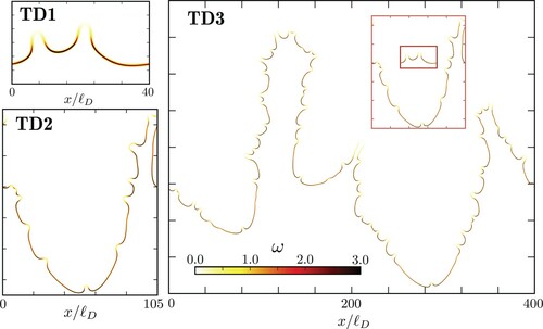
Figure 1 shows the reaction rate fields of the three TD flames. A visual inspection reveals a ubiquitous small scale unsteady thermo-diffusive cellular corrugation. These cells are seemingly of constant size and exhibit preferential diffusion effects in terms of enhanced reaction rate where the flame is convex towards the flame mixture and vice versa. Berger et al. [3] pointed out that for lean hydrogen flames the average size of such cells is equal to the size of the most amplified wavelength, which is itself of the order of the flame thickness. In addition, a minimal scatter with respect to the average size was observed. As the domain is increased from simulation TD1 to TD2, large-scale, finger-like structures appear, where periodic coalescence of the finger-like structures is additionally observed. Their size, however, seems to remain essentially constant at the larger domain size of simulation TD3. A domain independence of spatial scales is thus achieved for a sufficiently large domain size, a finding that was observed both for hydrogen flames [3] as well as in the context of one-step chemistry [2,7].

Figure 1. Contour plot of the reaction rate ω, for a single realisation of each TD series flame. While the entire domains are shown in the lateral crosswise direction, only a portion of the domain in the streamwise (propagation) direction is shown. The red box insets in the TD3 panel represents the TD1 and TD2 flame at the same scale of TD3.

2.2. Multi-step chemistry dataset

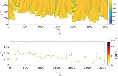
The dataset using detailed chemistry comprises a statistically planar, premixed, hydrogen/air flame in a rectangular two-dimensional computational domain, which is periodic in the crosswise direction. Snapshots of the non-dimensional temperature field θ and the heat release rate are shown in Figure 2. The non-dimensional temperature is defined as (1) $\theta =\frac{T-T_u}{T_{ad}-T_u},$(1) where $T_u$ is the temperature of the unburned mixture and $T_{ad}$ represents the adiabatic flame temperature. A constant inlet velocity of the unburned mixture (entering at the bottom of Figure 2) is chosen such that the flame is stabilised within the domain. The characteristic patterns arising from the thermo-diffusive instability mechanism have been discussed by Berger et al. [3], who identified a particular large-scale flame front corrugation (finger-like structures) in addition to the formation of small-scale cellular structures along the flame front. The conditions of the unburned mixture are set to an equivalence ratio of $\phi =0.4$, an unburned temperature $T_u=298$ K, and a pressure of p = 1bar.

Figure 2. Multi-step chemistry dataset of the hydrogen/air flame, spatial distribution: non-dimensional temperature (a) and heat release rate (b).

The flow is modelled by the reacting Navier–Stokes equations in the low-Mach limit [31] and the fluid is assumed to be an ideal gas. Species diffusivities are determined by imposing spatially homogeneous, non-unity Lewis numbers, which are computed in the burned gas, and the Soret effect, which is particularly relevant for hydrogen flames [32], is also considered. The reaction mechanism of Burke et al. [33] that contains 9 species and 46 reactions is used to model chemical reactions. A semi-implicit finite difference code based on the Crank–Nicolson time advancement scheme, an iterative predictor corrector scheme, and spatial and temporal staggering is employed [34]. Momentum equations are spatially discretised with a second-order scheme. Species and temperature equations are discretised with a third-order WENO scheme [35] and advanced by utilising Strang's operator splitting [36]. The mesh resolution and timestep size are chosen such that the laminar flame speed, heat release, temperature, and species profiles of a one-dimensional premixed unstretched flame computed by FlameMaster [37] are recovered adequately yielding a timestep size of 6 μs and a spatial resolution of ten grid points in the thermal flame thickness defined by the maximum gradient of temperature.

3. Manifolds dimensionality of thermo-diffusively unstable flames

3.1. Optimal estimator analysis

In the multi-step chemistry dataset, all length- and time-scales of the flow are resolved and assumptions related to the reduction of chemical mechanisms are avoided as a detailed reaction mechanism is used. Therefore, the dependency of the heat release with respect to all species and temperature can be rigorously studied. In particular, the heat release is defined as (2) $\dot{\omega }=\rho \sum _i{h}_i{\dot{\omega }}_i,$(2) where ρ represents the local density, $h_i$ represents the enthalpy of each species, ${\dot{\omega }}_i$ is the local rate of change of mass fraction of each species due to chemical reactions, and i denotes the summation index over all species. Thus, similar to the mass fraction source terms, the heat release is a high-dimensional function of species mass fractions $Y_i$ and temperature T, but, often, it can be well approximated by a lower-dimensional manifold, e.g. solely as function of the non-dimensional temperature θ.

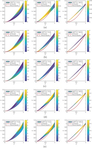
However, Regele et al. [38] have shown that in lean premixed hydrogen flames, the heat release cannot be well approximated solely as a function of the non-dimensional temperature and needs to be approximated by a higher dimensional manifold. The same issue has also been discussed in the context of other manifold methods such as FGM (flamelet generated manifolds) [39,40] and FPI (flame prolongation method of intrinsic low-dimensional manifolds) [41]. In particular, the heat release can be well described by two parameters, namely the non-dimensional temperature and mixture fraction Z or the non-dimensional temperature and the mass fraction of molecular hydrogen $Y_{H_2}$. The additional parameter (Z or $Y_{H_2}$) is required as lean premixed hydrogen flames are prone to thermo-diffusive instabilities, which cause a strong variation of the heat release along the flame front as a result of the strong differential diffusion of the hydrogen molecule. This leads to locally leaner and richer mixtures along the flame front and hence, induces strong heat release fluctuations. A closeup of the spatial distribution of the heat release in the flame is shown for the DNS in the left panel of Figure 3 (case $\mathrm{\Delta }=0$) and a detailed discussion about these fluctuations is provided by Berger et al. [3].

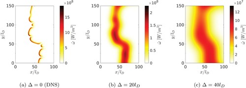
Figure 3. Closeup view of the large-scale flame shown in Figure 2: Spatial distribution of the unfiltered heat release and the filtered heat release for two different filter sizes, (a) $\mathrm{\Delta }=0$ (DNS), (b) $\mathrm{\Delta }=20l_D$, (c) $\mathrm{\Delta }=40l_D$.

The heat release varies along the flame front and hence, varies for constant values of the non-dimensional temperature and significant fluctuations are observed. In the context of optimal estimators these fluctuations can be quantified by the irreducible error, which measures the local fluctuations of $\dot{\omega }$ with respect to the conditional mean of the heat release with respect to the non-dimensional temperature $⟨\dot{\phantom{a}}\omega |\theta ⟩$. The conditional mean represents the optimal manifold to describe the heat release by the non-dimensional temperature alone; in case the irreducible error is small, the heat release can be well approximated by the non-dimensional temperature. Formally, the irreducible error is given as (3) ${ϵ}_{irr}^2=⟨(\dot{\omega }-⟨\dot{\omega }|\theta ⟩{)}^2⟩.$(3) Analogously, the local fluctuations with respect to higher dimensional manifolds can be determined by computing higher dimensional conditional averages, e.g. $⟨\dot{\phantom{a}}\omega |\theta ,C⟩$ if parametrising the heat release by the non-dimensional temperature θ and a progress variable C that is defined by means of the deficient reactant $Y_{H_2}$ as $C=1-Y_{H_2}$. To obtain a meaningful value, the irreducible error is normalised by the maximum value of the conditionally averaged heat release with respect to progress variable, yielding (4) ${ϵ}_{irr,norm}=\frac{\sqrt{{ϵ}_{irr}^2}}{max(⟨\dot{\omega }|\theta ⟩)}.$(4) It is worth noting that all irreducible errors, e.g. the one associated with the parametrisation by θ and the one related to the parametrisation by θ and C, are normalised with the same value '$max(⟨\dot{\phantom{a}}\omega |C⟩)$' to be comparable.

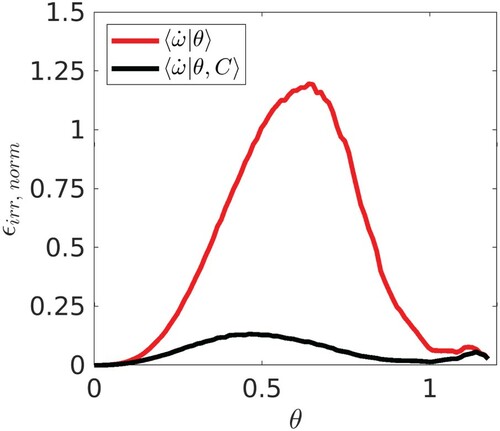
Figure 4 shows the irreducible error when using only the non-dimensional temperature for parametrisation and the irreducible error, averaged conditionally on θ, using the non-dimensional temperature and the progress variable for parametrisation. As described earlier, the parametrisation by only the non-dimensional temperature induces significant errors, which are above 100% for intermediate values of the non-dimensional temperature (at $\theta \approx 0.5$), as the local heat release fluctuations along the flame front cannot be captured. If using the non-dimensional temperature and the progress variable to parametrise the heat release, a significantly lower irreducible error is obtained indicating that the heat release may be represented by a two dimensional manifold such as $\dot{\omega }\approx f(\theta ,C)$. This result is consistent with the work of Regele et al. [38].

Figure 4. Irreducible errors for heat release parametrisation in the unfiltered case: comparison between the parametrisation based only on θ and the parametrisation based on θ and C.

3.2. The role of the LES filter

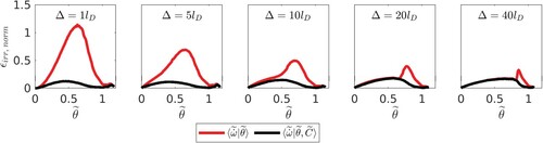
By means of the irreducible errors, the necessity for parametrising the heat release by the non-dimensional temperature and progress variable is evident from Figure 4. While using the unfiltered fields in the previous section, this section analyses the parametrisation of the filtered heat release $\tilde{\dot{\omega }}$ with respect to the filtered non-dimensional temperature $\tilde{\theta }$ and the filtered progress variable $\tilde{C}$ fields and, in particular, the effect of filter size variation on the parametrisation. The two-dimensional fields have been filtered by a Gauss filter [42]. A filter kernel $G\left(\overrightarrow{r}\right)$, defined as (5) $G\left(r\right)=\frac{6}{\pi {\mathrm{\Delta }}^2}\exp \left(-\frac{6r^2}{{\mathrm{\Delta }}^2}\right),$(5) is used, where $r=|\overrightarrow{x}-\overrightarrow{x}{}^{\prime }|$ refers to the distance of a point $\overrightarrow{x}{}^{\prime }$ with respect to the centre of the filter kernel $\overrightarrow{x}$ and Δ represents the filter size. In the following, the filter size Δ is measured in units of the laminar flame thickness $l_D$. The filtered field $\tilde{Q}$ of a generic variable Q, such as heat release, normalised temperature, and progress variable, is obtained by the following convolution integral: (6) $\tilde{Q}\left(\overrightarrow{x}\right)=\int G(|\overrightarrow{x}-\overrightarrow{x}{}^{\prime }|)Q\left(\overrightarrow{x}{}^{\prime }\right)\mathrm{d}\overrightarrow{x}{}^{\prime }.$(6) Figure 3 shows three closeups of the heat release of the multi-step chemistry dataset for different filter sizes. It can be seen that the fluctuations of the heat release along the flame front vanish for larger filter sizes and that a more uniform distribution along the flame front are observed.

Figure 5 shows the irreducible errors if parametrising the filtered heat release by $\tilde{\theta }$ or $\tilde{\theta },\tilde{C}$ for different filter sizes. It is worth noting that the maximum value of the conditionally averaged filtered heat release with respect to the non-dimensional temperature, $max(⟨\tilde{\dot{\omega }}|\tilde{\theta }⟩)$, which is used for the normalisation of the irreducible errors, changes for each filter size as the filtering procedure leads to a reduction of the filtered heat release values, c.f. also Figure 3. For small filter sizes and, in particular, for the unfiltered fields, significant irreducible errors are observed if using only the filtered non-dimensional temperature for parametrisation as observed in the previous section. Consistent with the spatial distributions of the filtered heat release in Figure 3, the discrepancy of irreducible errors if using $\tilde{\theta }$ or $\tilde{\theta },\tilde{C}$ reduces for larger filter sizes as the filtered heat release becomes more homogeneous along the flame front. Furthermore, the amplitude of the normalised irreducible errors reduces for large filter sizes, which indicates a reduction of the fluctuations of $\tilde{\dot{\omega }}$ with respect to the manifold $⟨\tilde{\dot{\omega }}|\tilde{\theta }⟩$. For instance, for the filter size of $\mathrm{\Delta }=40l_D$, the conditional error in Figure 5 is always below 30%. Hence, the filtered heat release may be modelled only based on $\tilde{\theta }$ for large filter sizes. Finding a suitable model that reflects this properties will be discussed in the remainder of this paper.

Figure 5. Irreducible errors for the parametrisation of the filtered heat release by sets based on the filtered progress variable and the filtered normalised temperature for different filter sizes.

4. A modelling framework based on filtered tabulated chemistry

In this section, building on the filtered tabulated chemistry approach, we introduce a subgrid modelling strategy for thermo-diffusively unstable, self-wrinkling premixed flames. First, the modelling approach is discussed and second, a-priori tested based on the one-step chemistry model DNS dataset introduced in Section 2.1. As mentioned in the introduction, the filtered tabulated approach utilises a lower dimensional manifold representation and in Section 3.1 it was established that thermo-diffusively unstable flames are best parametrised in terms of two independent parameters. The one-step model adopts an irreversible Arrhenius reaction model in which a deficient reactant is entirely depleted across the flame and thus determines the reaction rate. Such a formalism is natively a two-parameter model as the deficient reactant concentration, together with a nondimensional temperature are the only transported scalars.

4.1. Modelling strategy

The unfiltered deficient reactant system of governing equations is described in [17,19] and is comprised of two transport equations, respectively for the controlling reactant concentration Y, normalised with the unburned concentration $Y_u$, and for the nondimensional temperature θ. A progress variable based on the controlling reactant is also readily defined as C = 1−Y. The system of governing equations for the non-dimensional temperature θ and the progress variable C that are employed in the DNS with one-step chemistry can be filtered to obtain the following set of equations: (7) $\begin{array}{rl}\frac{\mathrm{\partial }\overline{\rho }\tilde{\theta }}{\mathrm{\partial }t}+\mathrm{\nabla }\cdot \left(\overline{\rho }\tilde{\mathbf{u}}\tilde{\theta }\right)& =-\mathrm{\nabla }\cdot (\overline{\rho }\widetilde{\mathbf{u}\theta }-\overline{\rho }\tilde{\mathbf{u}}\tilde{\theta })+\overline{\mathrm{\nabla }\cdot \left(\delta \mathrm{\nabla }\theta \right)+\frac{\omega }{\delta }}\end{array}$(7) (8) $\begin{array}{rl}\frac{\mathrm{\partial }\overline{\rho }\tilde{C}}{\mathrm{\partial }t}+\mathrm{\nabla }\cdot \left(\overline{\rho }\tilde{\mathbf{u}}\tilde{C}\right)& =-\mathrm{\nabla }\cdot (\overline{\rho }\widetilde{\mathbf{u}\mathbf{C}}-\overline{\rho }\tilde{\mathbf{u}}\tilde{C})+\overline{\mathrm{\nabla }\cdot \left(\frac{\delta }{Le}\mathrm{\nabla }C\right)+\frac{\omega }{\delta }}\end{array}$(8) where $\overline{\cdot }$ and $\tilde{\cdot }$ are, respectively, the spatial filtering and density-weighted filtering operations. Here spatial variables are made nondimensional with respect to the lateral domain size L, time is measured in units of $L/S_L^0$, ρ is the density in units of the unburned density ${\rho }_u$, $\delta ={\ell }_D/L$ is the nondimensional flame thickness, ω is the reaction rate and Le the Lewis number. In both equations, the two terms on the RHS are unclosed and are respectively the sub-grid scalar fluxes (SGSF) and the filtered flame front displacement (FFFD). The FFFD has been addressed in a previous study [7] for intrinsically unstable flames in the context of a flame surface density based approach. The FFFD consists of a filtered laminar diffusion term (FLDT) and a filtered reaction term (FRT) that will be discussed and modelled separately in the present work.

In this work, we model each of the unclosed terms by computing its conditional average with respect to $\tilde{\theta }$ and $\tilde{C}$ from a filtered DNS database. The terms are then represented as tabulated manifolds, using the two scalars $\tilde{\theta }$ and $\tilde{C}$ as table coordinates. Following the filtered tabulated approach and the F-TACLES formalism [14], the tables will have the LES filter size Δ as an additional parameter, and can be expressed for a generic variable as $\phi ={\phi }^{\ast }[\tilde{\theta },\tilde{C},\mathrm{\Delta }]$, where the ${}^{\ast }$ superscript denotes the quantities derived from a filtered dataset. The closure of each term is addressed in the following description:

• Filtered reaction rate The filtered reaction rate for temperature and progress variable are directly given by the filtered dataset: (9) $\overline{\omega }={\overline{\omega }}^{\ast }[\tilde{\theta },\tilde{C},\mathrm{\Delta }]$(9) where, as mentioned, the ${}^{\ast }$ superscript denotes the quantities directly established from a filtered dataset. Note that in the one-step chemistry DNS, the reaction rate can be directly expressed as a 2D table $\omega =\omega (C,\theta )$ with a simple analytical expression according to a one-step irreversible Arrhenius reaction [17,19].

• Filtered laminar diffusion terms These terms for both temperature and reactant are usually neglected or simply approximated as (10) $\begin{array}{rl}\overline{\mathrm{\nabla }\cdot \left(\delta \mathrm{\nabla }\theta \right)}& \approx \mathrm{\nabla }\cdot \left(\delta \mathrm{\nabla }\tilde{\theta }\right)\end{array}$(10) (11) $\begin{array}{rl}\overline{\mathrm{\nabla }\cdot \left(\frac{\delta }{Le}\mathrm{\nabla }C\right)}& \approx \mathrm{\nabla }\cdot \left(\frac{\delta }{Le}\mathrm{\nabla }\tilde{C}\right)\end{array}$(11) which is known to work well as long as the filter size remains on the order of the flame thickness. However, as the filter size becomes larger, significant errors can impact the prediction of the propagation speed. Following [14] corrective factors are introduced as follows: (12) $\begin{array}{rl}& {\alpha }_{\theta }[\tilde{\theta },\tilde{C},\mathrm{\Delta }]=\frac{|\overline{\mathrm{\nabla }\cdot \left(\delta \mathrm{\nabla }{\theta }^{\ast }\right)}|}{|\mathrm{\nabla }\cdot \left(\delta \mathrm{\nabla }\widetilde{{\theta }^{\ast }}\right)|},\end{array}$(12) (13) $\begin{array}{rl}& {\alpha }_C[\tilde{\theta },\tilde{C},\mathrm{\Delta }]=\frac{|\overline{\mathrm{\nabla }\cdot \left(\frac{\delta }{Le}\mathrm{\nabla }{C}^{\ast }\right)}|}{|\mathrm{\nabla }\cdot \left(\frac{\delta }{Le}\mathrm{\nabla }\widetilde{C^{\ast }}\right)|}.\end{array}$(13) As a result the unclosed terms can be written as (14) $\begin{array}{rl}\overline{\mathrm{\nabla }\cdot \left(\delta \mathrm{\nabla }\theta \right)}& =\mathrm{\nabla }\cdot \left({\alpha }_{\theta }\right[\tilde{\theta },\tilde{C},\mathrm{\Delta }\left]\delta \mathrm{\nabla }\tilde{\theta }\right)\end{array}$(14) (15) $\begin{array}{rl}\overline{\mathrm{\nabla }\cdot \left(\frac{\delta }{Le}\mathrm{\nabla }C\right)}& =\mathrm{\nabla }\cdot \left({\alpha }_C[\tilde{\theta },\tilde{C},\mathrm{\Delta }]\frac{\delta }{Le}\mathrm{\nabla }\tilde{C}\right)\end{array}$(15)

• Sub-grid scalar fluxes The SGSF is usually closed by means of gradient-type assumptions when the flow is characterised by elevated turbulence intensity. On the other hand, when turbulence is weak and the flow is dominated by the flame thermal expansion, counter-gradient type turbulent diffusion is usually expected [43]. In the present, self-wrinkling case, the SGSF are modelled, similarly to the correction factors, by the tables ${\mathrm{\Omega }}_{\theta }$ and ${\mathrm{\Omega }}_C$, again obtained by filtering the dataset using a Gaussian filter: (16) $\begin{array}{rl}{\mathrm{\Omega }}_{\theta }[\tilde{\theta },\tilde{C},\mathrm{\Delta }]& =-\mathrm{\nabla }\cdot ({\overline{\rho }}^{\ast }\widetilde{{\mathbf{u}}^{\mathbf{\ast }}{\theta }^{\mathbf{\ast }}}-{\overline{\rho }}^{\ast }{\tilde{\mathbf{u}}}^{\ast }{\tilde{\theta }}^{\ast })\end{array}$(16) (17) $\begin{array}{rl}{\mathrm{\Omega }}_C[\tilde{\theta },\tilde{C},\mathrm{\Delta }]& =-\mathrm{\nabla }\cdot ({\overline{\rho }}^{\ast }\widetilde{{\mathbf{u}}^{\mathbf{\ast }}{\mathbf{C}}^{\mathbf{\ast }}}-{\overline{\rho }}^{\ast }\widetilde{{\mathbf{u}}^{\mathbf{\ast }}}{\tilde{C}}^{\ast }).\end{array}$(17)

Note that the terms related to the filtered equation of state, continuity and momentum governing equations are not considered in the present analysis. Indeed, their role will be considered and assessed in the context of the envisaged a-posteriori studies on the same flame configurations.

4.2. Summary of the filtered equations

The filtered governing equations for the non-dimensional temperature and the progress variable can now be written in a closed form, using Equations (9(9) $\overline{\omega }={\overline{\omega }}^{\ast }[\tilde{\theta },\tilde{C},\mathrm{\Delta }]$(9) ), (12(12) $\begin{array}{rl}& {\alpha }_{\theta }[\tilde{\theta },\tilde{C},\mathrm{\Delta }]=\frac{|\overline{\mathrm{\nabla }\cdot \left(\delta \mathrm{\nabla }{\theta }^{\ast }\right)}|}{|\mathrm{\nabla }\cdot \left(\delta \mathrm{\nabla }\widetilde{{\theta }^{\ast }}\right)|},\end{array}$(12) ), (13(13) $\begin{array}{rl}& {\alpha }_C[\tilde{\theta },\tilde{C},\mathrm{\Delta }]=\frac{|\overline{\mathrm{\nabla }\cdot \left(\frac{\delta }{Le}\mathrm{\nabla }{C}^{\ast }\right)}|}{|\mathrm{\nabla }\cdot \left(\frac{\delta }{Le}\mathrm{\nabla }\widetilde{C^{\ast }}\right)|}.\end{array}$(13) ), (16(16) $\begin{array}{rl}{\mathrm{\Omega }}_{\theta }[\tilde{\theta },\tilde{C},\mathrm{\Delta }]& =-\mathrm{\nabla }\cdot ({\overline{\rho }}^{\ast }\widetilde{{\mathbf{u}}^{\mathbf{\ast }}{\theta }^{\mathbf{\ast }}}-{\overline{\rho }}^{\ast }{\tilde{\mathbf{u}}}^{\ast }{\tilde{\theta }}^{\ast })\end{array}$(16) ), (17(17) $\begin{array}{rl}{\mathrm{\Omega }}_C[\tilde{\theta },\tilde{C},\mathrm{\Delta }]& =-\mathrm{\nabla }\cdot ({\overline{\rho }}^{\ast }\widetilde{{\mathbf{u}}^{\mathbf{\ast }}{\mathbf{C}}^{\mathbf{\ast }}}-{\overline{\rho }}^{\ast }\widetilde{{\mathbf{u}}^{\mathbf{\ast }}}{\tilde{C}}^{\ast }).\end{array}$(17) ), as (18) $\begin{array}{rl}\frac{\mathrm{\partial }\overline{\rho }\tilde{\theta }}{\mathrm{\partial }t}+\mathrm{\nabla }\cdot \left(\overline{\rho }\tilde{\mathbf{u}}\tilde{\theta }\right)& ={\mathrm{\Omega }}_{\theta }[\tilde{\theta },\tilde{C},\mathrm{\Delta }]+\mathrm{\nabla }\cdot \left({\alpha }_{\theta }\right[\tilde{\theta },\tilde{C},\mathrm{\Delta }\left]\delta \mathrm{\nabla }\tilde{\theta }\right)+\frac{{\overline{\omega }}^{\ast }[\tilde{\theta },\tilde{C},\mathrm{\Delta }]}{\delta }\end{array}$(18) (19) $\begin{array}{rl}\frac{\mathrm{\partial }\overline{\rho }\tilde{C}}{\mathrm{\partial }t}+\mathrm{\nabla }\cdot \left(\overline{\rho }\tilde{\mathbf{u}}\tilde{C}\right)& ={\mathrm{\Omega }}_C[\tilde{\theta },\tilde{C},\mathrm{\Delta }]+\mathrm{\nabla }\cdot \left({\alpha }_C[\tilde{\theta },\tilde{C},\mathrm{\Delta }]\frac{\delta }{Le}\mathrm{\nabla }\tilde{C}\right)+\frac{{\overline{\omega }}^{\ast }[\tilde{\theta },\tilde{C},\mathrm{\Delta }]}{\delta }\end{array}$(19) where the filtered reaction term (FRT) is the same for the $\tilde{\theta }$ and $\tilde{C}$ transport equations while the sub grid scalar fluxes (SGSF) and the filtered diffusive terms (FLDT) differ between the two equations.

It is now of interest to inspect the tables generated from a representative thermal-diffusively unstable flame, using as table coordinates the filtered temperature and progress variable. For the present discussion as well as for the a-priori analysis presented in the next section, three representative LES filter sizes have been selected and applied to the one-step chemistry dataset, namely $\mathrm{\Delta }/{\ell }_D\sim 1,5,20$, respectively referred to as fine, medium and coarse.

Figure 6 displays the tables representing the values of the unclosed terms of Equations (18(18) $\begin{array}{rl}\frac{\mathrm{\partial }\overline{\rho }\tilde{\theta }}{\mathrm{\partial }t}+\mathrm{\nabla }\cdot \left(\overline{\rho }\tilde{\mathbf{u}}\tilde{\theta }\right)& ={\mathrm{\Omega }}_{\theta }[\tilde{\theta },\tilde{C},\mathrm{\Delta }]+\mathrm{\nabla }\cdot \left({\alpha }_{\theta }\right[\tilde{\theta },\tilde{C},\mathrm{\Delta }\left]\delta \mathrm{\nabla }\tilde{\theta }\right)+\frac{{\overline{\omega }}^{\ast }[\tilde{\theta },\tilde{C},\mathrm{\Delta }]}{\delta }\end{array}$(18) ) and (19(19) $\begin{array}{rl}\frac{\mathrm{\partial }\overline{\rho }\tilde{C}}{\mathrm{\partial }t}+\mathrm{\nabla }\cdot \left(\overline{\rho }\tilde{\mathbf{u}}\tilde{C}\right)& ={\mathrm{\Omega }}_C[\tilde{\theta },\tilde{C},\mathrm{\Delta }]+\mathrm{\nabla }\cdot \left({\alpha }_C[\tilde{\theta },\tilde{C},\mathrm{\Delta }]\frac{\delta }{Le}\mathrm{\nabla }\tilde{C}\right)+\frac{{\overline{\omega }}^{\ast }[\tilde{\theta },\tilde{C},\mathrm{\Delta }]}{\delta }\end{array}$(19) ), obtained using the TD1 flame dataset and conditionally averaged on the filtered progress variable and temperature. Also shown are the loci, in the θ –C space, of both the filtered and unfiltered flamelet profiles obtained from a 1D unstretched laminar flame. As the filter size is increased, it appears that $\tilde{\theta }$ and $\tilde{C}$ become increasingly correlated with a profile slope indicating that an effective Lewis number is approaching unity, as discussed in Section 3.2. For the larger filter size, the filtered 1D flamelet is observed to cover a similar parameter region in the 2D tables. This, however, hardly means that a filtered unstretched 1D flamelet is sufficient as a closure model, which is discussed in the following section, where the a-priori testing of the model is performed.

Figure 6. Visualisation of the tables representing the subfilter models for the unclosed terms, generated using the TD1 flame data. Each row represents the same term at three filter sizes while the tables are colour-coded by the value of the term. Superimposed on the tables is the locus in the θ-C space of both the filtered and unfiltered flamelet profiles obtained from a 1D unstretched laminar flame. (a) Filtered reaction rate, (b) Temperature filtered laminar diffusion term, (c) Progress variable filtered laminar diffusion term, (d) Temperature sub-grid scalar flux, (e) Progress variable sub-grid scalar flux.

5. A-priori testing of the proposed modelling framework

In this section, the proposed modelling framework is a-priori tested using the one-step chemistry dataset. The use of a one-step chemistry dataset allows us to discuss the model performance for filtered quantities without introducing any additional model uncertainty due to residual detailed chemistry effects. In fact, the unfiltered reaction rates of the one-step chemistry data are exactly represented by two scalars, while modelling errors are low but non-zero if representing the unfiltered reaction rates of the multi-step data by two scalars.

5.1. A-priori modelling of a small scale flame TD1

A first a-priori analysis is carried out on the TD1 flame by comparing the exact fields such as the reaction rate, extracted from the filtered DNS, with the modelled filtered reaction rate $\overline{\omega }$ using different strategies. More precisely, the modelled filtered reaction rate fields have been reconstructed using the following three types of tables: (i) a 2D table obtained using the conditional averages with respect to $\tilde{\theta }$ and $\tilde{C}$ and extracted from the TD1 flame itself, consistently with the framework described in Section 4, and denoted as 2Dtables-TD1; (ii) a 1D table using the conditional averages to $\tilde{C}$ extracted from the TD1 flame, and denoted as 1Dtables-TD1; (iii) a 1D table obtained by filtering a 1D unstretched laminar flamelet, denoted as 1Dtables-flamelet. The a-priori analysis is carried out in a standard manner, by a preliminary filtering operation of the DNS data (TD1 flame in this case), using a Gaussian filter with size Δ, thus yielding $\tilde{C}$ and $\tilde{\theta }$ and subsequently applying the model tables.

Results of the analysis on the small scale TD1 flame are shown in Figure 7 for the three representative filter sizes previously introduced. Regardless of the filter size, the modelled reaction rate based on a 2D table obtained using averages conditioned to $\tilde{\theta }$ and $\tilde{C}$ of the TD1 flame, almost perfectly matches the filtered DNS fields. This result is in agreement with the analysis carried out with the multi-step chemistry dataset in Section 3. Conversely, the performance of the other two models which are based on a 1D tabulation is rather different for each filter size.

Figure 7. A-priori analysis on filtered reaction rate $\overline{\omega }$ for the TD1 flame: comparison between filtered DNS, a-priori reconstructed field using 2D tables generated from TD1 flame simulation data and 1D filtered flamelets: (a) Fine LES filter $\mathrm{\Delta }=1{\ell }_D$, (b) Medium LES filter $\mathrm{\Delta }=5{\ell }_D$, (c) Coarse LES filter $\mathrm{\Delta }=20{\ell }_D$.

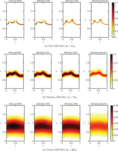
Figure 7(a) shows that, for the fine LES filter, neither of the 1D tabulation methods are able to represent the locally resolved complex weakening and strengthening behaviour of $\overline{\omega }$ occurring in the presence of strong two-dimensional curvature effects at the flame cusp tips and troughs. However, moving to larger filter sizes, as displayed in Figures 7(b,c), the two 1D tabulation methods show rather different modelling performances. The 1Dtables-TD1 model, shown in the third column, being based on the TD1 flame is able to correctly represent the filtered DNS fields for both the medium and coarse filter sizes. This confirms that the filtered flame structure is essentially one-dimensional, hence it can be described by a single-parameter manifold. This occurring once the inherently 2D morphological features due to the thermal-diffusive instability fall at the subfilter level. This is also evident from the irreducible error analysis of Figure 5 and confirms the interpretation given for the large filter sizes in the analysis of the tables of Figure 6. However, the 1Dtables-flamelet method, based on a 1D (one-parameter) tabulation of the filtered unstretched 1D flamelet profile, which is essentially the standard F-TACLES model [14], is not able to reproduce the filtered DNS for neither medium nor coarse filter sizes. This occurs because the unstretched 1D flamelet is unable to capture neither the complex flame features nor the net flame stretch effect that thermo-diffusive instabilities have on terms such as the filtered reaction rate. This is indicative of potentially relevant modelling errors that may arise in LES of themodiffusively unstable flames, when using tables derived from a filtered 1D unstretched flame.

At this stage, we note that modelling a small scale flame such as TD1 is only a proof of concept test of the modelling framework, which needs to be tested on a large flame, such as TD3. The idea, therefore, is to model a very large-scale flame such TD3 (or indeed one such as that shown in Figure 2), using tables obtained from smaller flames (ideally far smaller) that can be computed at a reasonable cost as an LES preprocessing step. In this context, we could consider as a reasonable cost the simulation of flames on the order of TD1 and TD2. This cost will be invariably higher than that of building standard flamelet libraries. However, it will be still rather small compared to the computational cost of an LES of a lab-scale device and possibly much smaller than that of an LES of an industrial-scale device.

5.2. A-priori modelling of a large scale flame TD3

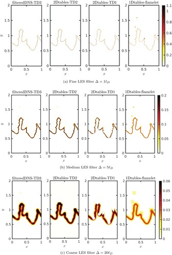
In this section, we perform an a-priori analysis by filtering the TD3 flame, using the same filter sizes as in the previous analysis. The filtered reaction rates from the TD3 DNS (referred to here as FilteredDNS-TD3) are then compared to the filtered reaction rate obtained by the following models:

• 2Dtables-TD2 This model is based on 2D filtered tables constructed using the conditional averages of an intermediate flame, namely TD2, larger than TD1.

• 2Dtables-TD1 This model is based on 2D filtered tables constructed using conditional averages from the TD1 flame.

• 1Dtables-flamelet This model is based on a 1D table obtained by filtering an unstretched laminar flamelet solution as done in [14].

Note that the second and third model of the previous list are the same models used in the a-priori analysis of the TD1 flame shown in Figure 7.

Figure 8 shows a visual comparison between the filtered reaction rate from the TD3 DNS (leftmost column) and the corresponding fields reconstructed using the above models. The 2Dtables-TD2 model is shown to correctly reproduce the filtered TD3 DNS fields for all three filters, with only minor differences that can be observed for the coarse filter size. An interesting feature is that for the fine filter size, for which the small scale wrinkling of the flame is resolved, the model is able to correctly reproduce quenching at the flame cusp tips and flame strengthening at the troughs. On the other hand, the 2Dtables-TD1 model reveals some modelling errors at each filter size analysed. Some of the flame regions, showing as white voids in the figure, cannot be reconstructed as the $C-\theta$ domain spanned by the 2Dtables-TD1 model is only a subset of the actual domain spanned by the TD3 DNS data. This could be circumvented by an extrapolation procedure which, however, was not implemented here in order to highlight such inconsistencies. Second, the values of $\overline{\omega }$ along the flame front appear to be lower than the filtered TD3 DNS, this possibly and ultimately leading to an underestimation of the overall consumption speed. The reason for this can be ascribed to the fact that the TD1 flame exhibits a statistically lower (positive) flame stretch than the TD3 and TD2 flames, thus leading, because of the Le<1 condition, to lower average reaction rates. Yet lower values of $\overline{\omega }$ are obtained by the 1D-flamelet model, which similarly to the case of sec 5.1, is not able to represent the complex behaviour of the filtered flame.

Figure 8. A-priori analysis on filtered reaction rate $\overline{\omega }$ for the TD3 flame. Comparison between filtered-DNS, and the three models: 2D tables constructed using the conditional averages of the filtered TD2 fields (2Dtables-TD2); 2D tables constructed using the conditional averages of the filtered TD2 fields (2Dtables-TD1); 1D filtered table of an unstretched laminar flamelet (1D-flamelet), (a) Fine LES filter $\mathrm{\Delta }=1{\ell }_D$, (b) Medium LES filter $\mathrm{\Delta }=5{\ell }_D$, (c) Coarse LES filter $\mathrm{\Delta }=20{\ell }_D$.

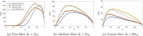
A more quantitative description for the filtered reaction term FRT is given in Figure 9 which displays the a-priori analysis on TD3 by means of conditional averages with respect to $\tilde{C}$. As expected from the spatial distribution of $\overline{\omega }$ previously discussed, for the fine and medium LES filters the 2Dtables-TD2 model is able to reproduce the filteredDNS-TD3 profiles across $\tilde{C}$ with a minimal error. Some discrepancies between the 2Dtables-TD2 model and the filteredDNS-TD3 are observed, however, for the coarse LES filter. The 2Dtables-TD1 model, on the other hand, is shown to underestimate the FRT for all the filter sizes employed in the analysis, while being able to correctly reproduce the qualitative shape of the FRT profiles across $\tilde{C}$. Conversely the 1Dtables-flamelet model introduces large quantitative discrepancies in the FRT profiles, in the order of up to 100%, as well as qualitative errors in the shape profile. Only for the largest filter size, while still exhibiting a pronounced quantitative discrepancy, 1Dtables-flamelet is capable of correctly recover the shape of the FRT profile, this being due to the amply discussed fact that when coarsely filtered, the flame exhibits a structure that can be described with one parameter.

Figure 9. A-priori analysis on filtered reaction term FRT ${\overline{\omega }}^{\ast }/\delta$ for the TD3 flame with three different filter sizes $\mathrm{\Delta }/{\ell }_D\sim 1,5,20$. Comparison between filtered-DNS, and the models: 2D tables constructed using the conditional averages of the filtered TD2 fields (2Dtables-TD2); 2D tables constructed using the conditional averages of the filtered TD1 fields (2Dtables-TD1); 1D filtered table of an unstretched laminar flamelet (1D-flamelet), (a) Fine filter $\mathrm{\Delta }=1{\ell }_D$, (b) Medium filter $\mathrm{\Delta }=5{\ell }_D$, (c) Coarse filter $\mathrm{\Delta }=20{\ell }_D$.

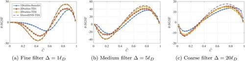
Similar considerations can be drawn observing the a-priori analysis on the SGSF conditional averages reported in Figure 10 for the progress variable and in Figure 11 for the temperature. The two SGSF profiles show rather similar behaviour and shape across $\tilde{C}$ with comparable values for both the medium and coarse filter sizes. Also in this case the 2Dtables-TD2 is shown to be more accurate in reproducing the SGSF of both C and θ, compared to 2Dtables-TD1 and 1Dtables-flamelet models. This confirming once again that, while the 2Dtables-TD2 model requires a more expensive preprocessing step for building the tables, it increases the modelling capabilities of the proposed framework. In particular, the key feature of the TD2 dataset that leads to the excellent performances of the 2Dtables-TD2 model is the presence of at least one large scale flame finger in the simulated domain, as shown in Figure 1, which is otherwise absent on a smaller domain such as TD1. The morphological feature represented by flame fingers and the ensuing flame stretch pattern can be therefore considered as a requisite for a minimal flame unit to correctly represent a large scale flame such as TD3. Residual errors may then be attributed to the absence, in such minimal flame unit, of more elaborate, but maybe less relevant features such as the interaction between adjacent flame fingers, visible in TD3.

Figure 10. A-priori analysis on subgrid scalar flux SGSF of C for the TD3 flame with three different filter sizes $\mathrm{\Delta }/{\ell }_D\sim 1,5,20$. Comparison between filtered-DNS, and the three models: 2D tables constructed using the conditional averages of the filtered TD2 fields (2Dtables-TD2); 2D tables constructed using the conditional averages of the filtered TD1 fields (2Dtables-TD1); 1D filtered table of an unstretched laminar flamelet (1D-flamelet), (a) Fine filter $\mathrm{\Delta }=1{\ell }_D$, (b) Medium filter $\mathrm{\Delta }=5{\ell }_D$, (c) Coarse filter $\mathrm{\Delta }=20{\ell }_D$.

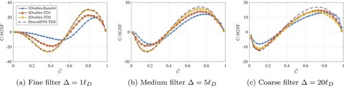
Figure 11. A-priori analysis on subgrid scalar flux SGSF of θ for the TD3 flame with three different filter sizes $\mathrm{\Delta }/{\ell }_D\sim 1,5,20$. Comparison between filtered-DNS, and the three models: 2D tables constructed using the conditional averages of the filtered TD2 fields (2Dtables-TD2); 2D tables constructed using the conditional averages of the filtered TD1 fields (2Dtables-TD1); 1D filtered table of an unstretched laminar flamelet (1D-flamelet), (a) Fine filter $\mathrm{\Delta }=1{\ell }_D$, (b) Medium filter $\mathrm{\Delta }=5{\ell }_D$, (c) Coarse filter $\mathrm{\Delta }=20{\ell }_D$.

In conclusion, this a-priori analysis has shown promising results for the 2Dtables-TD2 model, in the context of subfilter modelling of thermo-diffusively unstable flames in a laminar setting. However, the extension of such an approach to a turbulent scenario is not trivial (see for instance the discussion in [7] in the context of flame surface density modelling of thermodiffusively unstable flames). Following the standard F-TACLES approach, a possible solution that can be examined is to resort to an additional turbulent wrinkling factor model. The complex interplay of intrinsic instability and turbulence, however, may lead to different conclusions than the ones found in this study with respect to the most suitable subgrid model.

6. Conclusion

In this paper, a data-driven, subfilter modelling framework for thermo-diffusively unstable premixed flames, such as lean hydrogen-air flames, has been discussed. The study is based on data gathered from fully resolved, statistically planar, two-dimensional simulations of thermo-diffusively unstable flames exhibiting multi-scale self-wrinkling. It has been assessed, by means of an optimal estimator analysis performed on large scale two-dimensional lean hydrogen flames, that such unsteady corrugated deflagrative fronts are characterised with good accuracy by two parameters, i.e. by a thermochemical manifold parametrised by two independent variables. A modelling framework based on the filtered tabulated chemistry approach is suggested and, on the basis of data collected from a filtered, fully resolved simulation, tables for all unclosed terms as a function of two variables as well as the filter size are constructed. To illustrate this framework, a one-step, deficient-reactant model is used based on a progress variable and a non-dimensional temperature. Tables for the filtered reaction term, filtered laminar diffusion terms and subgrid scalar fluxes are assembled for different filter sizes by filtering fully resolved simulations. Two simulations of small and medium sizes are used to develop two distinct models, which are then a-priori tested on a third larger-size simulation. Additional models are also tested, based on one-parameter representations of the flame structure. The two-parameter model based on the medium size simulation was found to be the most accurate as it best represents the complex multi-scale, unsteady, stretched character of thermo-diffusively unstable flames. The model based on the small size simulation, while still sufficiently accurate, was observed to be lacking some of the large-scale morphological features typical of thermo-diffusively unstable flames, thus introducing some error. The least accurate models were found to be those based on one-dimensional manifolds. In particular, a one-parameter model based on fully resolved simulations was observed to perform well only for large filter sizes, while a model based on a filtered one-dimensional unstretched flame was observed to introduce large errors for all filter sizes.

The proposed modelling framework is expected to be effective in a wide range of thermochemical conditions, provided the two-dimensional, self-wrinkling flames are simulated at the same conditions as the target case. Future work will be dedicated to the modelling of 3D, turbulent, lean hydrogen or hydrogen enriched hydrocarbon flames. Efforts will also be focalised on the a-posteriori testing of such modelling framework on laboratory burner configurations.

Acknowledgments

F. Creta and N. Fogla wish to express the greatest gratitude to M. Matalon for his support and guidance over the years. L. Berger and H. Pitsch gratefully acknowledge generous support of the European Research Council (ERC) under the European Union's Horizon 2020 research and innovation program (grant agreement No. 695747).

Disclosure statement

No potential conflict of interest was reported by the author(s).

Additional information

Funding

L. Berger and H. Pitsch gratefully acknowledge generous support of the European Research Council (ERC) under the European Union's Horizon 2020 research and innovation program (grant agreement No. 695747).

References

- Matalon M., Flame dynamics, Proc. Combust. Inst. 32 (2009), pp. 57–82. doi: https://doi.org/10.1016/j.proci.2008.08.002
- F. Creta, P.E. Lapenna, R. Lamioni, N. Fogla, and M. Matalon, Propagation of premixed flames in the presence of Darrieus–Landau and thermal diffusive instabilities. Combust. Flame 216 (2020), pp. 256–270. doi: https://doi.org/10.1016/j.combustflame.2020.02.030
- Berger L., Kleinheinz K., Attili A., and Pitsch H., Characteristic patterns of thermodiffusively unstable premixed lean hydrogen flames, Proc. Combust. Inst. 37(2) (2019), pp. 1879–1886. doi: https://doi.org/10.1016/j.proci.2018.06.072
- Shanbhogue S.J., Sanusi Y.S., Taamallah S., Habib M.A., Mokheimer E.M.A., and Ghoniem A.F., Flame macrostructures, combustion instability and extinction strain scaling in swirl-stabilized premixed CH4/H2 combustion, Combust. Flame 163 (2016), pp. 494–507. doi: https://doi.org/10.1016/j.combustflame.2015.10.026
- Chterev I. and Boxx I., Effect of hydrogen enrichment on the dynamics of a lean technically premixed elevated pressure flame, Combust. Flame 225 (2021), pp. 149–159. doi: https://doi.org/10.1016/j.combustflame.2020.10.033
- Hawkes E.R. and Chen J.H., Direct numerical simulation of hydrogen-enriched lean premixed methane air flames, Combust. Flame 138 (2004), pp. 242–258. doi: https://doi.org/10.1016/j.combustflame.2004.04.010
- Lapenna P.E., Lamioni R., and Creta F., Subgrid modeling of intrinsic instabilities in premixed flame propagation, Proc. Combust. Inst. 38 (2021), pp. 2001–2011. doi: https://doi.org/10.1016/j.proci.2020.06.192
- SB. Pope, Small scales, many species and the manifold challenges of turbulent, Proc. Combust. Inst.34 (2013), pp. 1–31. doi: https://doi.org/10.1016/j.proci.2012.09.009
- Wu H. and Ihme M., Compliance of combustion models for turbulent reacting flow simulations, Fuel186 (2016), pp. 853–863. doi: https://doi.org/10.1016/j.fuel.2016.07.074
- Balarac G., Pitsch H., and Raman V., Development of a dynamic model for the subfilter scalar variance using the concept of optimal estimators, Phys. Fluids 20 (2008), pp. 035114.
- Berger L., Kleinheinz K., Attili A., Bisetti F., Pitsch H., and Mueller M.E., Numerically accurate computational techniques for optimal estimator analyses of multi-parameter models, Comb. Model.22(3) (2018), pp. 480–504. doi: https://doi.org/10.1080/13647830.2018.1424353
- Molkov V., Makarov D., and Grigorash A., Cellular structure of explosion flames, modeling and large-eddy simulation, Comb. Sci. Tech. 176 (2004), pp. 851–865. doi: https://doi.org/10.1080/00102200490428495
- Keppeler R., Tangermann E., Allaudin U., and Pfitzner M., LES of low to high turbulent combustion in an elevated pressure environment, Flow Turbulence Combust. 92 (2014), pp. 767–802. doi: https://doi.org/10.1007/s10494-013-9525-1
- Fiorina B., Vicquelin R., Auzillon P., Darabiha N., Gicquel O., and Veynante D., A filtered tabulated chemistry model for LES of premixed combustion, Combust. Flame 157 (2010), pp. 465–475. doi: https://doi.org/10.1016/j.combustflame.2009.09.015
- Vreman A.W., van Oijen J.A., de Goey L.P.H., and Bastiaans R.J.M., Subgrid scale modeling in large-Eddy simulation of turbulent combustion using premixed flamelet chemistry, Flow Turbulence Combust. 82 (2009), pp. 511–535. doi: https://doi.org/10.1007/s10494-008-9159-x
- Lapenna P.E., Lamioni R., Troiani G., and Creta F., Large scale effects in weakly turbulent premixed flames, Proc. Combust. Inst. 37(2) (2019), pp. 1945–1952. doi: https://doi.org/10.1016/j.proci.2018.06.154
- Creta F., Lamioni R., Lapenna P.E., and Troiani G., Interplay of Darrieus–Landau instability and weak turbulence in premixed flame propagation, Phys. Rev. E 94(5) (2016), p. 053102. doi: https://doi.org/10.1103/PhysRevE.94.053102
- Lamioni R., Lapenna P.E., Troiani G., and Creta F., Strain rates, flow patterns and flame surface densities in hydrodynamically unstable, weakly turbulent premixed flames, Proc. Combust. Inst. 37(2) (2019), pp. 1815–1822. doi: https://doi.org/10.1016/j.proci.2018.06.196
- Lamioni R., Lapenna P.E., Troiani G., and Creta F., Flame induced flow features in the presence of Darrieus–Landau instability, Flow Turb. Combust. 101(4) (2018), pp. 1137–1155. doi: https://doi.org/10.1007/s10494-018-9936-0
- Lapenna P.E. and Creta F., Mixing under transcritical conditions: an a-priori study using direct numerical simulation, J. Supercrit. Fluids 128 (2017), pp. 263–278. doi: https://doi.org/10.1016/j.supflu.2017.05.005
- Lapenna P.E., Lamioni R., Ciottoli P.P., and Creta F., Low-Mach Number Simulations of Transcritical Flows AIAA-paper 2018-0346 (2018).
- Lapenna P.E., Characterization of pseudo-boiling in a transcritical nitrogen jet, Phys. Fluids 30(7) (2018), p. 077106. doi: https://doi.org/10.1063/1.5038674
- Lapenna P.E. and Creta F., Direct numerical simulation of transcritical jets at moderate reynolds number, AIAA J. 57(6) (2019), pp. 2254–2263. doi: https://doi.org/10.2514/1.J058360
- Patera A.T., A spectral element method for fluid dynamics: laminar flow in a channel expansion, J. Comput. Phys. 54(3) (1984), pp. 468–488. doi: https://doi.org/10.1016/0021-9991(84)90128-1
- Fischer P.F., Lottes J.W., and Kerkemeier S.G., nek5000 web page, http://nek5000.mcs.anl.gov (2008).
- Matalon M. and Bechtold J.K., Hydrodynamic theory of premixed flames: effects of stoichiometry, variable transport coefficients and arbitrary reaction orders, J. Fluid Mech. 487 (2003), pp. 179–210. doi: https://doi.org/10.1017/S0022112003004683
- Creta F. and Matalon M., Propagation of wrinkled turbulent flames in the context of hydrodynamic theory, J. Fluid Mech. 680 (2011), pp. 225–264. doi: https://doi.org/10.1017/jfm.2011.157
- Matalon M. and Matkowsky B.J., Flames as gasdynamic discontinuities, J. Fluid Mech. 124 (1982), pp. 239–259. doi: https://doi.org/10.1017/S0022112082002481
- Attili A., Lamioni R., Berger L., Kleinheinz K., Lapenna P.E., Pitsch H., and Creta F., The effect of pressure on the hydrodynamic stability limit of premixed flames, Proc. Combust. Inst. 38 (2021), pp. 1973–1981. doi: https://doi.org/10.1016/j.proci.2020.06.091
- Lamioni R., E.Lapenna P., Berger L., Kleinheinz K., Attili A., Pitsch H., and Creta F., Pressure-induced hydrodynamic instability in premixed methane-Air slot flames, Combust. Sci. Technol. 192 (2020), pp. 1998–2009. doi: https://doi.org/10.1080/00102202.2020.1768081
- Tomboulides A., Lee J., and Orszag S., Numerical simulation of low mach number reactive flows, J. Scientif. Comput. 12 (1997), pp. 139–167. doi: https://doi.org/10.1023/A:1025669715376
- Zhou Z., Hernandez-Perez F.E., Shoshin Y., van Oijen J.A., and de Goey L.P.H., Effect of soret diffusion on lean hydrogen/air flames at normal and elevated pressure and temperature, Combust. Theor. Model. 21 (2017), pp. 879–896. doi: https://doi.org/10.1080/13647830.2017.1311028
- Burke M.P., Chaos M., Ju Y., Dryer F.L., and Klippenstein S.J., Comprehensive H2/O2 kinetic model for high-Pressure combustion, Int. J. Chem. Kinet. 44 (2012), pp. 444–474. doi: https://doi.org/10.1002/kin.20603
- Desjardins O., Blanquart G., Balarac G., and Pitsch H., High order conservative finite difference scheme for variable density low mach number turbulent flows, J. Comput. Phys. 227 (2008), pp. 7125–7159. doi: https://doi.org/10.1016/j.jcp.2008.03.027
- Jiang G.S. and Shu C.W., Efficient implementation of weighted ENO schemes, J. Comput. Phys.126 (1996), pp. 202–228. doi: https://doi.org/10.1006/jcph.1996.0130
- Strang G., On the construction and comparison of difference schemes, SIAM J. Numer. Anal. 5 (1968), pp. 506–517. doi: https://doi.org/10.1137/0705041
- Pitsch H., FlameMaster, a C++ computer program for 0D combustion and 1D laminar flame calculations.
- Regele J.D., Knudsen E., Pitsch H., and Blanquart G., A two-equation model for non-unity lewis number differential diffusion in lean premixed laminar flames, Combust. Flame 160 (2013), pp. 240–250. doi: https://doi.org/10.1016/j.combustflame.2012.10.004
- de Swart J.A.M., Bastiaans R.J.M., van Oijen J.A., de Goey L.P.H., and Cant R.S., Inclusion of preferential diffusion in simulations of premixed combustion of hydrogen/Methane mixtures with flamelet generated manifolds, Flow Turb. Combust. 85 (2010), pp. 473–511. doi: https://doi.org/10.1007/s10494-010-9279-y
- Vreman A.W., van Oijen J.A., de Goey L.P.H., and Bastiaans R.J.M., Direct numerical simulation of hydrogen addition in turbulent premixed bunsen flames using flamelet-generated manifold reduction, Int. J. Hydrogen Energy 34 (2009), pp. 2778–2788. doi: https://doi.org/10.1016/j.ijhydene.2009.01.075
- Gicquel O., Darabiha N., and Thevenin D., Laminar premixed hydrogen/air counterflow flame simulations using flame prolungation of ILDM with differential diffusion, Proc. Combust. Inst. 28 (2000), pp. 1901–1908. doi: https://doi.org/10.1016/S0082-0784(00)80594-9
- S. Pope, Turbulent flows, Cambridge University Press, Cambridge, UK, 2000.
- Veynante D., Trouve A., Bray K.N.C., and Mantel T., Gradient and counter-gradient scalar transport in turbulent premixed flames, J. Fluid Mech. 332 (1997), pp. 263–293. doi: https://doi.org/10.1017/S0022112096004065