Asymptotic analysis of detonation development at SI engine conditions using computational singular perturbation

Abstract

The occurrence and intensity of the detonation phenomenon at spark-ignition (SI) engine conditions is investigated, with the objective to successfully predict super-knock and to elucidate the effect of kinetics and transport at the ignition front. The computational singular perturbation (CSP) framework is employed in order to investigate the chemical and transport mechanisms of deflagration and detonation cases in the context of 2D high-fidelity numerical simulations. The analysis revealed that the detonation development is characterised by: (i) stronger explosive dynamics and (ii) enhanced role of convection. The role of chemistry was also found to be pivotal to the detonation development which explained the stronger explosive character of the system, the latter being an indication of the system's reactivity. The role of convection was found to be enhanced at the edge of the detonating front. Moreover, the increased contribution of convection was found to be related mainly to heat convection. Remarkably, the detonation front was mainly characterised by dissipative and not explosive dynamics. Finally, diffusion was found to have negligible role to both examined cases.

Keywords:

• detonation
• super-knock
• CSP
• explosive dynamics

1. Introduction

To meet the increasing demands of lower carbon footprint, the current engine technology needs to be significantly improved in terms of both efficiency and emissions, with flexibility in fuels derived from petroleum or renewable sources. One approach towards this direction is a downsized IC engine [1] that can produce a comparable power to that of a larger engine through the use of different techniques: turbocharging or supercharging, often coupled with direct injection (DI), advanced exhaust gas recirculation (EGR) or variable valve timing (VVT). The main benefits from the downsized engines are the increased thermal and fuel efficiencies [2, 3] and the inherent high-power density [4]. It has been demonstrated that a downsized and boosted engine with an optimal injection strategy can achieve very high gross thermal efficiency of 48.7% with 21 bar gross indicated mean effective pressure (IMEP) [5]. Downsized engines have been reported to successfully mitigate CO${}_2$ emissions by reducing fuel consumption [6], making it a serious contender in reducing greenhouse emissions and harmful pollutants [1]. When matched with technologies, advanced IC engines such as homogeneous charge compression ignition (HCCI)-type combustion also allow considerable fuel flexibility. Particularly, they can operate not only with conventional gasoline- and diesel-like fuels, but also with alternative or renewable fuels, such as natural gas, ethanol, methanol, and biodiesel [5, 7].

However, one of the major technical challenges in downsized and boosted engines is the pre-ignition, and even super-knock [8]. The pre-ignition phenomenon refers to a premature autoignition of the reactant mixture prior to the spark ignition timing due to various ignition sources [9, 10], triggering end-gas autoignition, and subsequently it may induce deflagration-to-detonation (DDT) transition. This leads to extremely high-peak amplitudes of pressure oscillations in the combustion chamber, and consequently causes severe mechanical damage [11]. Optical diagnostics carried out by Wang et al. [8] showed that the mechanism of super-knock is described as hot spot-induced DDT followed by high-pressure oscillation. Detonation develops if there is a coherent coupling between the acoustic wave and the reaction front [12, 13]. At these conditions, the front speed and the peak pressure are comparable to the Chapman-Jouguet (CJ) detonation speed, and the von Neumann pressure $P_{\mathrm{ZND}}$ spike, respectively [14].

Considering its practical significance, many engineering strategies to suppress pre-ignition and super-knock have been reported. Gong et al. [15] demonstrated a successful implementation of an early or late secondary injection, resulting in a decreased super-knock frequency, fuel consumption, and emissions, while $N{O}_x$ level was found to be increased. Dai et al. [16] also reported that local $N{O}_x$ concentrations play a role in detonation development in dimethyl ether (DME)/air mixtures within negative temperature coefficient (NTC) regime, in engines using EGR. The attenuation of fuel reactivity was also considered. Liu et al. [17] performed experiments with rapid compression machine (RCM), where replacing part of gasoline fuel with less reactive methane or propane was found to transition the combustion mode from detonation to flame propagation. They also reported that methanol was effective in suppressing detonation development. The effect of spark location and timing was also found to have an impact [18], such that advancing the spark timing was found to induce super-knock at high compression ratio conditions [14, 19].

Fundamental description of the ignition and detonation development has also been studied extensively. Since the theoretical classification of ignition regimes by Zel'dovich [12], Bradley and co-workers [20–22] proposed the regime diagram to identify the detonation propensity in the presence of two non-dimensional parameters based on the reactivity of the mixture and the temperature distribution in the hot spot. A number of one-dimensional simulations were conducted to reproduce the ‘detonation peninsula’ for a specific choice of fuels [23–25].

Sow et al. [26] also reported that the temperature gradient in the bulk mixture affects the run-up time and intensity of the detonation. Luong et al. [27] extended the theory into multidimensional direct numerical simulations to characterise the ignition behaviour in the presence of turbulence intensity and temperature fluctuations and thoroughly validated by statistical analysis.

Extensive experimental and numerical studies by the engine research community have provided valuable insights into the detonation mechanism [14]. Quantitative and qualitative results obtained from many optical diagnostics and high-fidelity numerical simulations under IC engine conditions greatly help develop and validate the theoretical predictive models of engine knock [28–30]. Experiments, however, provide only limited access to detailed spatial and temporal information on temperature, pressure, and individual species of the developing detonation process [31]. They fail to provide detailed information on the interplay of the chemical reactions and their respective timescales, and convection and diffusion associated with super-knock conditions, and the relative role of the temperature over the evolution of the system. On the contrary, direct numerical simulation (DNS) can provide more detailed information associated with the complex flow and species fields [27]. A systematic and rigorous diagnostic tool is therefore needed to extract salient information from massive DNS datasets, and thus provide a better understanding of the dynamics of the developing detonation such as the interplay between the relevant transport processes and dominant chemical pathways.

Based on the geometric singular perturbation (GSP) concept introduced in the 1970s [32], the computational singular perturbation (CSP) is an algorithmic method of asymptotic analysis developed by Lam and Goussis [33], initially applied in problems of chemical kinetics [34] and later extended to other fields, such as reacting flows [35, 36], biology [37], pharmacokinetics [38] and others. In problems of reacting flows with detailed chemistry, CSP allows a characterisation of dynamical structures and their properties in the phase space, by identifying the fastest timescales that become quickly exhausted to equilibrium, thus establishing certain constraints called slow invariant manifolds (SIM), on which the system dynamics evolve at fast and slow active timescales. The simplified form of the governing equations produces the reduced model, which governs the flow along the SIM. Specifically, CSP allows the decomposition of the system to a range of modes, i.e. mathematical objects each characterised by two features: an amplitude (dictating the impact to the system's slow evolution) and a timescale (indicating the time-frame of action). Based on the magnitudes of these features and the nature of each mode (i.e. explosive versus dissipative), the investigator can identify algorithmically the mode(s) being most important to the system's slow evolution. The physical interpretation is then obtained by using mathematical formulas which enable the identification of the important physical processes (chemical reactions or transport processes) that contribute to the mode(s) amplitude or the timescales.

The objective of this study is to apply the CSP algorithm and various tools in order to identify key changes in the system's dynamics and to examine the interplay between transport processes (convective and diffusive) and chemistry towards the development of detonation phenomena. The results from this examination aim to shed more light into a highly complex phenomenon that despite being a topic of research for many decades our understanding is yet limited. The analysis is based on data produced by two-dimensional simulations representing engine conditions, investigated under two distinguished events with and without detonation occurrence.

2. Material and methods

2.1. Numerical setup

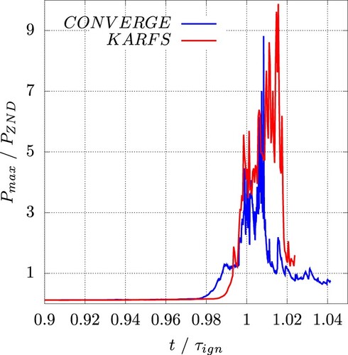
CONVERGE software [39] was utilised for simulating two 2D cases, representative of SI engine conditions, carried out on Shaheen II supercomputer at KAUST. The soundness of CONVERGE CFD as a tool to model detonation has been verified with an incompressible code, KARFS [40, 41], and the results of this benchmarking exercise are presented in Appendix.

CONVERGE CFD software is used for engine applications with the capability to capture detonation phenomena [18, 42–45]. To advance in time, the fully compressible formulation of the Navier-Stokes, energy and species equations, a pressure-implicit with splitting of operator (PISO) algorithm is used. The Redlich-Kwong equation of state is used with mixture-averaged diffusion coefficients, suitable for high-temperature, high-pressure conditions and accounting for real gas behaviour. High-resolution simulations were run in the direct numerical simulation (DNS) mode without turbulence submodels, with detailed chemical reaction terms solved by the Multi-Zone Well-Stirred Reactor (MZ-WSR) model [46], fully coupled with the flow solver. The time advancement is performed with a variable timestep, 1st order implicit Euler, limited by Courant–Friedrichs–Lewy (CFL) number for Mach of 1.0, with $\mathrm{\Delta }{t}_{min}$ ranging from 5e−10 to 5e−09 s. For the boundary conditions, the four boundaries are represented as solid walls at which no-slip velocity and zero-gradient conditions for scalar variables are imposed. The spatial discretization is handled by the monotonic upstream-centred scheme for conservation laws (MUSCL), providing a 2nd order of accuracy for the convection term. The diffusion terms in the transport equation are discretised using a 2nd order central difference scheme.

In all cases, a square 2D domain was employed with dimensions of $20.464\times 20.464\mathrm{mm}$ as in Refs. [7, 27, 47, 48]. The domain is made up of a base grid of size of 32 µ m with level 2 adaptive mesh refinement (AMR) computed at every timestep, yielding the minimum grid size of 8 µ m. As shown in Table 1, a Gaussian hot spot with distribution $\sigma =1\mathrm{mm}$ representing the spark plug in an SI engine is imposed at the centre of the left domain boundary, and its resolution is further improved by setting up a level 3 fixed embedding (FE) over it, at $r=5\mathrm{mm}$, yielding a local cell refinement of 4 µ m. The maximum temperature of the hot spot is set at $T_{max}=1400\mathrm{K}$, representing practical engine conditions. Two cases were considered; Case A is representative of detonation (supersonic behaviour), while Case B is representative of deflagration (subsonic behaviour). The distinct combustion modes allow a direct comparison between the two cases through which the unique features associated with the detonation dynamics are revealed.

Table 1. Summary of the numerical setup.

Simulation setup	Characteristics
Domain	$20.464\times 20.464\mathrm{mm}$
Grid	$32\times 32\mathrm{mu}\mathrm{m}$, AMR level 2
Gaussian hot spot	$T_{max}=1400\mathrm{K}$, $\sigma =1\mathrm{mm}$, Fixed Embedding scale 3, $r=5\mathrm{mm}$
Temperature field	$T_{\mathrm{mean}}=1100\mathrm{K}$, $\mathrm{\Delta }{T}_{\mathrm{RMS}}=5\mathrm{K}$, $l_T=5\mathrm{mm}$, 1.5 mm
Pressure	$P_{\mathrm{in}}=35\mathrm{atm}$
Reactive fuel	C${}_2$H${}_5$OH, $\phi =1$
Chemical mechanism	40 species, 180 elementary reactions

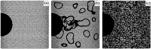
Figure 1 displays the mesh resolution at the initial timestep (a), $t_0$, for both cases and at the timestep of 99% ${\tau }_{\mathrm{ign}}$ for Cases A and B ((b) and (c)), where ${\tau }_{\mathrm{ign}}$ is the homogeneous ignition delay time. It is shown that the grid refinement increases significantly in the areas of high temperature gradients. At the very initial timestep, this area is near the hot spot, while as time evolves autoigniting kernels emerge and the AMR algorithm adds the grid refinement accordingly.

Figure 1. Grid resolution after AMR and FE refinement at (a) $t_0$ for both Cases A and B, (b) 99% ${\tau }_{\mathrm{ign}}$ for Case A and (c) 99% ${\tau }_{\mathrm{ign}}$ for Case B, where ${\tau }_{\mathrm{ign}}$ is the homogeneous ignition delay time.

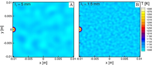
In addition, the inherent temperature inhomogeneity found in IC engines was addressed by imposing a temperature stratification in the mixture of uniform composition as the initial condition, as shown in Figure 2. The most energetic length scale of temperature fluctuation, $l_T$, is 5 mm and 1.5 mm for Cases A and B, respectively, and the temperature fluctuations in the domain were imposed by the root mean square (RMS) temperature $\mathrm{\Delta }{T}_{\mathrm{RMS}}=5\mathrm{K}$. The selected $l_T$ and $\mathrm{\Delta }{T}_{\mathrm{RMS}}$ values for Case A ensure the occurrence of detonation, as has been demonstrated in Refs. [7, 47]. The computational square domain has been chosen sufficiently large to accommodate four most energetic length scales of temperature fluctuations ($l_T$) in each direction, thereby reproducing the statistically significant behaviour of multiple ignition front interactions while also keeping the computational cost affordable.

Figure 2. Temperature fields for Case A (left) and Case B (right) at the initial timestep $t_0$.

The initial pressure, $P_{\mathrm{in}}$ in both cases was set at 35 atm, representing the case of the in-cylinder pressure at the top dead centre (TDC), while the von Neumann pressure $P_{\mathrm{ZND}}$ based on the initial mean temperature is 34.8 MPa, and the Chapman-Jouguet velocity $U_{\mathrm{CJ}}$ is 1834.2 m/s. Ethanol is chosen as a fuel because it is considered to be a representative non-NTC related renewable biodiesel. Additionally, due to the high autoignitive resistance provided by the high octane number (ON) of ethanol, triggering detonation in such conditions is physically harder. Therefore, the results of this study are applicable to fuels/blends at higher ON ratings. The chemical mechanism consists of 40 species and 180 elementary reactions [49]. The equivalence ratio of the bulk mixture is initially set to $\phi =1$. The strong detonation case (Case A) and the deflagration case (Case B) both have a mean temperature of 1100 K. The high bulk mixture temperatures of both cases aim to reflect the end gas autoignition conditions in order to reduce the computational cost, following the practice of Luong et al. [7, 47]. Concretely, the simulations herein only capture the onset of the end-gas autoignition event, where the remaining unburned fuel/air mixture has already been heated up to a high temperature and pressure. This allows for a good balance between computational expenses and fidelity of the simulations. Finally, since the end-gas autoignition occurs at a very short timescale (in the order of microseconds), the entire process is assumed to occur at a constant volume, thereby neglecting the effect of the piston movement.

2.2. Ignition regime characterisation

The Bradley ignition regime diagram was developed on the basis of a one-dimensional setup, but serves as a representative metric for the 2D simulations. The Bradley diagram employs two non-dimensional numbers, (ξ and ε), to identify the developing detonation peninsula, thus distinguishing the zones of subsonic and supersonic autoignitive fronts, as well as thermal explosion [21]. The ξ parameter is a non-dimensional number and represents the ratio of the speed of sound (a) to the propagation speed ($S_{\mathrm{sp}}$). (1) $\xi =a/S_{\mathrm{sp}}$(1) Note that the upper and lower ξ limits of the C-shaped curve of the developing detonation regime strongly depend on the initial conditions, fuel type, and the kinetic model used in the simulations [24, 25]. In general, a strong detonation development is expected when ξ ranges between 1 to $O(10)$ [24, 25], and for ξ values lower than unity homogeneous thermal explosion occurs. The ε parameter denotes the ratio of the residence time of the pressure wave in the radius of the autoignition kernel ($r_{\mathrm{hs}}$) to the excitation time (${\tau }_e$): (2) $\epsilon =(r_{\mathrm{hs}}/a)/{\tau }_e$(2) where ${\tau }_e$ is determined from the heat release rate profile at the reference mixture condition [21].

In multidimensional problems, the representative ξ in a uniform mixture with temperature inhomogeneities is approximated as $\xi \cong a|d{\tau }_{\mathrm{ign}}/\mathrm{dT}||\widetilde{\mathrm{\nabla T}}|$ [27, 31] where $\widetilde{\mathrm{\nabla }T}$ is the statistical mean temperature gradient and ${\tau }_{\mathrm{ign}}$ is the homogeneous ignition delay time at a local mixture condition.

In the isotropic temperature field fluctuations, Peters et al. [28] found that the characteristic length scale representing the size of hot spots $r_{\mathrm{hs}}$ is comparable with the mean distance of the dissipation elements, ${\overline{l}}_{\mathrm{DE}}$. As such, $\widetilde{\mathrm{\nabla }T}$ is approximated as $\widetilde{\mathrm{\nabla }T}\cong T_{\mathrm{RMS}}/{\overline{l}}_{\mathrm{DE}}$, where $T_{\mathrm{RMS}}$ the root-mean-square (RMS) temperature fluctuation. ${\overline{l}}_{\mathrm{DE}}$ is found to be approximately equal to a half of the two-point autocorrelation integral length scale, ${\overline{l}}_{\mathrm{DE}}\cong l_{\mathrm{et}}/2$, for the isotropic energy spectrum adopted in this study [27].

Similarly, ε for the multidimensional field is approximated as [27] (3) $\epsilon ={\overline{l}}_{\mathrm{DE}}/(l_m/\alpha ),$(3) where $l_m$ is the minimum run-up distance to form direct detonation initiation from a hot spot [50]. α is the weighting factor, $\alpha =4$, that accounts for the shortened run-up distance of detonation formation quantitatively observed in the DNS, resulting from the interaction and collision of multiple ignition fronts in the highly-reactive transient mixture conditions. More specifically, under the highly-reactive conditions of end-gas autoignition, it was found that the multi-dimensional effect of the interaction and collision of emerging multiple ignition kernels greatly promotes the onset of detonation, and thus shortens the run-up distance of detonation initiation as compared to that of 1D laminar detonation initiated by only an isolated hot spot [27, 50]. As quantitatively observed in the DNS cases, the weighting value of 4 was introduced to account for these effects [27].

The significance of ξ and ε is that no detonation is expected for $\epsilon \ll 1$ regardless of the magnitude of the ξ parameter. As ε approaches unity, the transient mixture state shifts towards the boundary of the detonation peninsula, and the developing detonation is expected. For $\epsilon \gg 1$ fully developed detonation is expected to occur for $\xi \sim$ 1 to $O(10)$ [27].

In this study, it was found that $\epsilon =1.3$ and $\xi =9.3$ for Case A, and $\epsilon =0.4$ and $\xi =31$ for Case B, thereby suggesting that Case A exhibits strong detonation as opposed to the non-detonating (deflagrative) Case B.

Note that the complex thermo-chemical and physical processes of the entire engine cycle are not reproduced in this study due to the expensive computational cost of DNS. However, the conditions of a high temperature and pressure, the most energetic length scale, and the temperature fluctuation of temperature considered in this study are configured to replicate the end-gas autoignition process that is typically observed near the top dead centre (TDC) of a SI engine. As such, the simulated results in this study are directly relevant to the behaviour of the detonation development process observed in an IC engine.

2.3. Computational singular perturbation (CSP) and its algorithmic tools

For complex chemical systems with a large number of species and reactions, an analytical tool is necessary in order to identify the smaller set of processes that are most essential in determining the system dynamics. A common approach is the local sensitivity analysis (LSA), which quantifies the importance of the individual model parameters on the evolution of the system by computing the sensitivity coefficients. This approach is unable to identify distinct characteristic times for individual processes and may sometimes lead to misleading results [51]. The principal component analysis (PCA) [52] is another common approach to reduce the dimensionality by transforming a large set of variables into a smaller one that preserves as much statistical information as possible [53]. Again, PCA is typically extracted from a large dataset throughout the entire evolution of the dynamical system, and hence does not capture the temporal aspects of the system.

In contrast, the computational singular perturbation (CSP) is an algorithmic method of asymptotic analysis that can be applied on any multiscale physical system to identify different dynamical modes with characteristic time scales. Through the construction of the basis chemical eigenvectors, CSP transforms the n-dimensional (where n is the number of reactive scalars) coupled systems into n characteristic modes with distinct eigenvalues that are ordered by magnitude. This allows an identification of the fast modes that are exhausted to steady state, while the remaining slow modes evolves on the low dimensional manifolds at much larger timescales. More recently, the tangential stretching rate (TSR) was defined as a weighed sum of all relevant eigenvalues and mode amplitudes as a unified scalar metric to describe the explosive/dissipative nature of the system evolving on the manifolds [54, 55].

The details of the CSP method used herein and its algorithmic tools have been discussed elsewhere (see for instance [56–58]), and only a brief summary is provided here. Following the standard practice, vectors are denoted by boldface letters. Consider the system of species and temperature governing equations in the general form of Equation (4(4) $\frac{\mathrm{\partial }\mathbf{z}}{\mathrm{\partial }t}={\mathbf{L}}_T(\mathbf{z})+\mathbf{g}(\mathbf{z}),{\mathbf{L}}_T(\mathbf{z})={\mathbf{L}}_C(\mathbf{z})+{\mathbf{L}}_D(\mathbf{z})$(4) ): (4) $\frac{\mathrm{\partial }\mathbf{z}}{\mathrm{\partial }t}={\mathbf{L}}_T(\mathbf{z})+\mathbf{g}(\mathbf{z}),{\mathbf{L}}_T(\mathbf{z})={\mathbf{L}}_C(\mathbf{z})+{\mathbf{L}}_D(\mathbf{z})$(4) where $\mathbf{z}$ is the system's (N + 1)-dimensional state vector that includes the N mass fractions of the chemical species ($y_1,y_2,\dots ,y_N$) and temperature (T), ${\mathbf{L}}_D(\mathbf{z})$, ${\mathbf{L}}_C(\mathbf{z})$, ${\mathbf{L}}_T(\mathbf{z})$ the (N + 1)-dimensional vectors representing the spatial transport operators for diffusion, convection and their sum, respectively, and g(z) the (N + 1)-dimensional vector of the chemical source term. In the absence of any spatial inhomogeneities (i.e. ${\mathbf{L}}_T(\mathbf{z})=\mathbf{0}$) Equation (4(4) $\frac{\mathrm{\partial }\mathbf{z}}{\mathrm{\partial }t}={\mathbf{L}}_T(\mathbf{z})+\mathbf{g}(\mathbf{z}),{\mathbf{L}}_T(\mathbf{z})={\mathbf{L}}_C(\mathbf{z})+{\mathbf{L}}_D(\mathbf{z})$(4) ) degenerates to Equation (5(5) $\frac{\mathrm{\partial }\mathbf{z}}{\mathrm{\partial }t}=\mathbf{g}(\mathbf{z}),{\mathbf{L}}_T(\mathbf{z})=\mathbf{0}$(5) ): (5) $\frac{\mathrm{\partial }\mathbf{z}}{\mathrm{\partial }t}=\mathbf{g}(\mathbf{z}),{\mathbf{L}}_T(\mathbf{z})=\mathbf{0}$(5) According to the CSP framework, the system of Equation (4(4) $\frac{\mathrm{\partial }\mathbf{z}}{\mathrm{\partial }t}={\mathbf{L}}_T(\mathbf{z})+\mathbf{g}(\mathbf{z}),{\mathbf{L}}_T(\mathbf{z})={\mathbf{L}}_C(\mathbf{z})+{\mathbf{L}}_D(\mathbf{z})$(4) ) can be transformed to Equation (6(6) $\frac{\mathrm{\partial }\mathbf{z}}{\mathrm{\partial }t}=\sum _{i=1}^{N+1}{\mathit{a}}_i{h}^i,h^i={\mathit{b}}^i({\mathit{L}}_T+\mathit{g})$(6) ): (6) $\frac{\mathrm{\partial }\mathbf{z}}{\mathrm{\partial }t}=\sum _{i=1}^{N+1}{\mathit{a}}_i{h}^i,h^i={\mathit{b}}^i({\mathit{L}}_T+\mathit{g})$(6) where ${\mathit{a}}_i$, ${\mathit{b}}^i$ the i-th dual (row and column, respectively) CSP basis vectors, so that ${\mathit{b}}^j{\mathit{a}}_i={\delta }_i^j$. In essence, CSP allows us to decompose the state vector to a set of (N + 1) CSP modes, by projecting the original system to the directions of the eigenmodes. The CSP basis vectors can be calculated through an iterative refinement process or, as it will be discussed next, they can be approximated by the eigenvectors of the Jacobian of the chemical source term. Each CSP mode is characterised by a timescale ${\tau }_i$ and an amplitude $h^i$; the former dictates the frame of action of the i-th mode, while the latter defines its impact on the system's slow evolution [59]. Although the CSP modes and the associated timescales and amplitudes are purely mathematical objects, physical meaning can be obtained by examining the process (and in certain cases the variables) that contribute the most to their generation. Note that the CSP analysis is neither restricted by specific flowcharacteristics, e.g. compressible/incompressible or subsonic/supersonic, and no adjustment in the analysis is necessary for the present study of detonation problem. The flow characteristics are reflected on the transport terms in the transport equations and hence are inherently represented by the amplitudes of the CSP modes.

Some of the modes (j<M) are much faster than the remaining (slow) ones and the temporal evolution of the whole system. Hence, the M fast timescales become quickly exhausted, allowing the projection of the original system onto the slow invariant manifolds. The system is confined to evolve on a manifold under the action of the remaining $((N+1)-M)$ slow (active) modes, described by: (7) $\frac{\mathrm{\partial }\mathbf{z}}{\mathrm{\partial }t}\approx \sum _{i=M}^{N+1}{\mathit{a}}_i{h}^i,h^j\approx 0,j=1,\dots M$(7) For leading order accuracy, the CSP basis vectors ${\mathit{a}}_i$, ${\mathit{b}}^i$ can be approximated by the right and left eigenvectors ${\mathit{\alpha }}_i$, ${\mathit{\beta }}^i$, respectively, of the Jacobian J of the chemical source term $\mathit{g}(\mathit{z})$ [60, 61]. Then, the i-th timescale ${\tau }_i$ can be calculated on the basis of the respective eigenvalue ${\lambda }_i$, i.e. ${\tau }_i=\frac{1}{|{\lambda }_i|}$. The sign of the eigenvalue (positive or negative) determines the nature of the respective CSP mode; a negative eigenvalue indicates a dissipative mode that tends to drive the system towards equilibrium, while a positive eigenvalue is called explosive [62] that drives the system away from the equilibrium. For example, when dissipative modes dominate, the right-hand-side RHS of Equation (4(4) $\frac{\mathrm{\partial }\mathbf{z}}{\mathrm{\partial }t}={\mathbf{L}}_T(\mathbf{z})+\mathbf{g}(\mathbf{z}),{\mathbf{L}}_T(\mathbf{z})={\mathbf{L}}_C(\mathbf{z})+{\mathbf{L}}_D(\mathbf{z})$(4) ) decays while when an explosive mode dominates the RHS of Equation (4(4) $\frac{\mathrm{\partial }\mathbf{z}}{\mathrm{\partial }t}={\mathbf{L}}_T(\mathbf{z})+\mathbf{g}(\mathbf{z}),{\mathbf{L}}_T(\mathbf{z})={\mathbf{L}}_C(\mathbf{z})+{\mathbf{L}}_D(\mathbf{z})$(4) ) increases exponentially. Explosive modes have been extensively investigated in reacting flows because they are inherently related to limit phenomena and flames. As previously discussed, however, their mere existence does not qualify them as dominant ones for the system's slow evolution. In fact, their action may be largely cancelled by the action of other more active dissipative modes, hence their net effect can be insignificant. In any case, their consideration as dominant ones has to always be subject to investigation. In fact, according to Equation (7(7) $\frac{\mathrm{\partial }\mathbf{z}}{\mathrm{\partial }t}\approx \sum _{i=M}^{N+1}{\mathit{a}}_i{h}^i,h^j\approx 0,j=1,\dots M$(7) ), two conditions must be satisfied in order for a mode to have a strong effect on the system's slow evolution [63]: (i) its timescale ${\tau }_i$ must be among the fastest of the slow ones, i.e. ${\tau }_{M+1}\le {\tau }_i\le {\tau }_{M+k}$, where k>1 but sufficiently small, and (ii) its amplitude $h^i$ must be the largest one in magnitude (or at least sufficiently close to the largest one). Throughout the manuscript, ‘explosive’ character is represented by the existence of CSP modes with their associated eigenvalues being positive.

To assess the contribution of each physical process (chemical or transport-related) to the development of the i-th amplitude $h^i$, the amplitude participation index (API) is used [64]. For a chemical source term expressed as Equation (8(8) $\mathit{g}(\mathit{z})=\sum _{k=1}^{2K}{\hat{\mathit{S}}}_k{R}^k$(8) ): (8) $\mathit{g}(\mathit{z})=\sum _{k=1}^{2K}{\hat{\mathit{S}}}_k{R}^k$(8) where ${\hat{\mathit{S}}}_k$ the (N + 1)-dimensional generalised stoichiometric vector of the k-th reaction, $R^k$ the respective reaction rate and $2K$ the total number of unidirectional reactions, the amplitude $h^i$ is written in the form of Equation (9(9) $h^i={\mathit{\beta }}^i({\mathit{L}}_T+\mathit{g})=\sum _{j=1}^{N+1}{\beta }_j^i{L}_{T,j}+\sum _{k=1}^{2K}{\mathit{\beta }}^i{\hat{\mathit{S}}}_k{R}^k=\sum _{m=1}^{2K+N+1}{\gamma }_m^i$(9) ): [65]: (9) $h^i={\mathit{\beta }}^i({\mathit{L}}_T+\mathit{g})=\sum _{j=1}^{N+1}{\beta }_j^i{L}_{T,j}+\sum _{k=1}^{2K}{\mathit{\beta }}^i{\hat{\mathit{S}}}_k{R}^k=\sum _{m=1}^{2K+N+1}{\gamma }_m^i$(9) Then, the API is defined as Equation (10(10) $P_k^n=\frac{{\gamma }_k^n}{\sum _{m=1}^{2K+N+1}|{\gamma }_m^n|}$(10) ): (10) $P_k^n=\frac{{\gamma }_k^n}{\sum _{m=1}^{2K+N+1}|{\gamma }_m^n|}$(10) thereby measuring the contribution of the k-th process to the n-th CSP mode [66]. The signs of the eigenvectors ${\mathit{\alpha }}_i$, ${\mathit{\beta }}_i$ are properly adapted in order to ensure that the amplitudes of all slow (active) modes are positive. The positive API values then indicate that the associated processes enhance the impact of the respective mode while the opposite holds for negative API values.

An additional tool recently developed in the CSP framework is the tangential stretching rate (TSR) [54, 55], which is the resultant effect of all eigenvalues with weights that depend on the amplitudes of the modes, i.e. (11) ${\omega }_{{\tilde{\tau }}_{R+T}}=\sum _{i=M+1}^{N+1}{W}_{i,R+T}{\lambda }_i,W_{i,R+T}=\frac{h^i}{L_T+g}\sum _{k=M+1}^{N+1}\frac{h^k}{L_T+g}$(11) where $L_T$ and g the norms of ${\mathit{L}}_T$ and $\mathit{g}$, respectively. In the absence of any spatial inhomogeneities, Equation (11(11) ${\omega }_{{\tilde{\tau }}_{R+T}}=\sum _{i=M+1}^{N+1}{W}_{i,R+T}{\lambda }_i,W_{i,R+T}=\frac{h^i}{L_T+g}\sum _{k=M+1}^{N+1}\frac{h^k}{L_T+g}$(11) ) leads to Equation (12(12) ${\omega }_{{\tilde{\tau }}_R}=\sum _{i=M+1}^{N+1}{W}_{i,R}{\lambda }_i,W_{i,R}=\frac{h^i}{g}\sum _{k=M+1}^{N+1}\frac{h^k}{g}$(12) ): (12) ${\omega }_{{\tilde{\tau }}_R}=\sum _{i=M+1}^{N+1}{W}_{i,R}{\lambda }_i,W_{i,R}=\frac{h^i}{g}\sum _{k=M+1}^{N+1}\frac{h^k}{g}$(12) Note that in the above definition, TSR only considers the action of the slow (active) modes.

As such, the TSR on the basis of Equation (11(11) ${\omega }_{{\tilde{\tau }}_{R+T}}=\sum _{i=M+1}^{N+1}{W}_{i,R+T}{\lambda }_i,W_{i,R+T}=\frac{h^i}{L_T+g}\sum _{k=M+1}^{N+1}\frac{h^k}{L_T+g}$(11) ) is called reactive-transport TSR while that from Equation (12(12) ${\omega }_{{\tilde{\tau }}_R}=\sum _{i=M+1}^{N+1}{W}_{i,R}{\lambda }_i,W_{i,R}=\frac{h^i}{g}\sum _{k=M+1}^{N+1}\frac{h^k}{g}$(12) ) is reactive TSR, to reflect the presence or absence of the transport process in the formulation [67, 68]. Furthermore, due to the large dynamic range of values that both ${\omega }_{{\tilde{\tau }}_{R+T}}$ and ${\omega }_{{\tilde{\tau }}_R}$ obtain, they are both represented in logarithms, i.e.: (13) ${\mathrm{\Omega }}_{R+T}=\mathrm{Sign}({\omega }_{{\tilde{\tau }}_{R+T}})\cdot \mathrm{Lo}{g}_{10}|{\omega }_{{\tilde{\tau }}_{R+T}}|,{\mathrm{\Omega }}_R=\mathrm{Sign}({\omega }_{{\tilde{\tau }}_R})\cdot \mathrm{Lo}{g}_{10}|{\omega }_{{\tilde{\tau }}_R}|$(13) In the following analysis, the system's fast explosive eigenvalue (${\lambda }_{e,f}$) is similarly logarithmically scaled, i.e. ${\mathrm{\Lambda }}_{e,f}=\mathrm{Lo}{g}_{10}{\lambda }_{e,f}$. To avoid clutters, values of ${\omega }_{{\tilde{\tau }}_{R+T}}$, ${\omega }_{{\tilde{\tau }}_R}$ and ${\lambda }_{e,f}$ less than unity are not presented because they bear little impact on the system's slow dynamics. Hence, positive and negative values of ${\mathrm{\Omega }}_{R+T}$ and ${\mathrm{\Omega }}_R$ denote explosive and dissipative dynamics. Recall that the ‘explosive’ TSR follows that introduced by CSP, implying that one or more positive eigenvalues have far bigger weights than the remaining negative eigenvalues. All physical timescales are normalised by a nominal time of 1 second, such that the magnitudes shown in the results are non-dimensional.

By definition, ${\mathrm{\Omega }}_{R+T}\approx {\mathrm{\Omega }}_R$ implies that the system becomes nearly homogeneous, hence the chemical reactions dominate the system dynamics. However, when ${\mathrm{\Omega }}_{R+T}\ne {\mathrm{\Omega }}_R$, no simple conclusion can be drawn for the relative significance of the transport and chemical reactions. In that case, an alternative approach is required, and the TSR amplitude participation index (TSR-API) provides valuable insights. The TSR-API is a weighted average of the API values of the k-th process from all active modes with weights that depend on the contribution of each mode to the construction of TSR, i.e. (14) $H_k^{R+T}={\mathit{V}}^{R+T}{\mathit{API}}_k$(14) where ${\mathit{V}}^{R+T}$ a ($(N+1)-M$) row vector which contains the weights of all active modes to ${\omega }_{{\tilde{\tau }}_{R+T}}$, i.e. (15) $V_n^{R+T}=\mathrm{Sign}(\mathrm{Re}({\lambda }_n))\cdot \frac{W_{n,R+T}|{\lambda }_n|}{\sum _{i=M+1}^{N+1}|W_{i,R+T}||{\lambda }_i|}$(15) and ${\mathit{API}}_k$ a ($(N+1)-M$) column vector containing the API values $P_k^n$ of the k-th process across all n active modes, ($n=M+1,\dots ,N+1$). Since the TSR-API tool $H_k^{R+T}$ is defined for both chemical reactions and transport-related processes, both effects are aggregated to obtain the net contribution of chemistry and transport to the magnitude and nature (dissipative or explosive) of the TSR (${\omega }_{{\tilde{\tau }}_{R+T}}$), i.e.: (16) $H_R^{R+T}=\sum _{k=1}^{2K}{H}_k^{R+T},H_D^{R+T}=\sum _{k=1}^{N+1}{H}_k^{R+T},H_C^{R+T}=\sum _{k=1}^{N+1}{H}_k^{R+T},H_T^{R+T}=\sum _{k=1}^{2(N+1)}{H}_k^{R+T}$(16) In the above Equation (16(16) $H_R^{R+T}=\sum _{k=1}^{2K}{H}_k^{R+T},H_D^{R+T}=\sum _{k=1}^{N+1}{H}_k^{R+T},H_C^{R+T}=\sum _{k=1}^{N+1}{H}_k^{R+T},H_T^{R+T}=\sum _{k=1}^{2(N+1)}{H}_k^{R+T}$(16) ), $H_R^{R+T}$, $H_D^{R+T}$, $H_C^{R+T}$, $H_T^{R+T}$ denote the overall contributions of chemistry, diffusion, convection and transport (i.e. both convection and diffusion), respectively, to ${\omega }_{{\tilde{\tau }}_{R+T}}$.

Note that the eigenvectors used in Equation (7(7) $\frac{\mathrm{\partial }\mathbf{z}}{\mathrm{\partial }t}\approx \sum _{i=M}^{N+1}{\mathit{a}}_i{h}^i,h^j\approx 0,j=1,\dots M$(7) ) (and subsequently in Equations (9(9) $h^i={\mathit{\beta }}^i({\mathit{L}}_T+\mathit{g})=\sum _{j=1}^{N+1}{\beta }_j^i{L}_{T,j}+\sum _{k=1}^{2K}{\mathit{\beta }}^i{\hat{\mathit{S}}}_k{R}^k=\sum _{m=1}^{2K+N+1}{\gamma }_m^i$(9) )–(16(16) $H_R^{R+T}=\sum _{k=1}^{2K}{H}_k^{R+T},H_D^{R+T}=\sum _{k=1}^{N+1}{H}_k^{R+T},H_C^{R+T}=\sum _{k=1}^{N+1}{H}_k^{R+T},H_T^{R+T}=\sum _{k=1}^{2(N+1)}{H}_k^{R+T}$(16) )) are produced on the basis of the chemical source terms solely while the transport terms are projected on to the directions produced by these basis vectors [35, 69, 70]. The rationale for this approach was that the system's stiffness is mainly introduced by the chemical source term. Evidence to corroborate that argument in laminar and turbulent flames was reported in [64, 71]. As such, it has been demonstrated that it is sufficient to compute the fast and slow basis vectors based on the chemical dynamics, and transport has negligible contribution. This will be clearly illustrated in the analysed results where it will be shown that chemistry largely dominates over transport.

In the following, for all presented results related to the CSP analysis, the CSPTk package [54, 72] integrated with the TChem [73] package for thermo-kinetic database management was employed.

3. Results and discussion

3.1. Overall combustion characteristics

To properly analyse the ignition dynamics of two distinct Cases A and B, which exhibit detonation development and regular deflagration, respectively, instantaneous data fields at comparable stages were selected for analysis in order to compare the evolution characteristics in both cases. Scaling the temporal evolution of both systems against the respective ignition delay times (determined on the basis of the maximum rate of change of the mean temperature), five instants ($t_1$–$t_5$) were selected as shown in Table 2.

Table 2. Timestep selection for Case A and Case B.

		Case A			Case B
Timestep		t [ms]	$P_{max}/P_{\mathrm{ZND}}$	$T_{\mathrm{mean}}$ [K]	t [ms]	$P_{max}/P_{\mathrm{ZND}}$	$T_{\mathrm{mean}}$ [K]
$t_1$	0.975${\tau }_{\mathrm{ign}}$	0.21999	0.16	1386.9	0.22167	0.15	1441.9
$t_2$	0.980${\tau }_{\mathrm{ign}}$	0.22112	0.32	1468.7	0.22281	0.17	1519.1
$t_3$	0.988${\tau }_{\mathrm{ign}}$	0.22292	0.96	1620.4	0.22463	0.21	1714.6
$t_4$	0.990${\tau }_{\mathrm{ign}}$	0.22337	1.26	1692.9	0.22508	0.25	1789.3
$t_5$	1.000${\tau }_{\mathrm{ign}}$	0.22563	3.37	2463.9	0.22736	0.65	2526.7

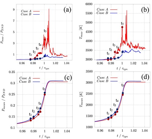
Figure 3 shows that the selected instants capture the critical moments as both the volume-averaged (mean) pressure ($P_{\mathrm{mean}}$) and temperature ($T_{\mathrm{mean}}$) evolve significantly during the ignition. Note that the mean pressure and temperature are both calculated by averaging all computational cells of the domain per timestep. In addition, for the detonating case, Case A, the first three instants are before the detonation onset, $t_4$ is immediately after the detonation onset and at $t_5$ the detonation event has evolved further. A time is referred to as ‘before’ or ‘after’ the detonation onset based on whether the local pressure normalised by the von Neumann pressure ($P_{\mathrm{ZND}}$) is less or greater than unity. Considering that $P_{\mathrm{ZND}}=34.8\mathrm{MPa}$ for both cases, Figure 3 shows that $P_{max}$ of Case A clearly exceeds $P_{\mathrm{ZND}}$, reaching $P_{max}/P_{\mathrm{ZND}}$ values of 9.7. In fact, at $t_3$ the pressure ratio is just below unity (value of 0.96) while at $t_4$ it has just become greater than unity (value of 1.26), and at $t_5$ it has increased further to 3.37. As will be shown next, the $P_{max}$ values detailed in Table 2 and Figure 3 all relate to the same ignition kernel. On the contrary, the pressure of Case B does not exceed $P_{\mathrm{ZND}}$, $P_{max}/P_{\mathrm{ZND}}<1$.

Figure 3. (a) Normalized maximum pressure; (b) Maximum temperature; (c) Normalized mean pressure; (d) Mean temperature. Red lines and markers denote Case A, blue lines and markers denote Case B. The respective values for Cases A and B are marked for the five time selections. For the exact values of the highlighted instants see Table 2.

To further assess the detonability of Case A, the temperature field at five selected instants is shown in Figure 4. A notable difference between the two cases is the significantly larger number of ignition kernels established in Case B, which is a direct consequence of the smaller $l_T$ of Case B compared to Case A (1.5 mm and 5.0 mm, respectively). Hence, in Case A larger high-temperature spots allow a longer run-up distance to develop detonation, resulting in favourable conditions for detonation [74]. On the other hand, in Case B the smaller $l_T$ leads to a larger number of smaller pockets of gas which autoignite concurrently. This results in less detonative, smaller spots unable to develop into detonation due to their competition with the consumption of the unburned fuel.

Figure 4. Temporal evolution of temperature contours for the five selected times for Case A (first row) and B (second row). In subfigures (a–c) of Case A, the red circle indicates the location where the detonation event is first established. For the details of the selected times see Table 2 and Figure 3.

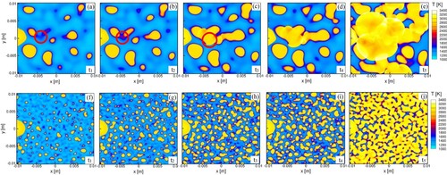
Figure 4 shows that the ignition kernels created in Case A develop further in time and undergo collision and merging, thereby establishing new and stronger ignition fronts. The merging of ignition fronts directly results in strengthening the associated pressure waves. Close-up views in Figure 5 clearly show that the detonation onset in Case A is a consequence of the shock-to-shock interaction among at least three ignition kernels which appear to merge at $t_3$ and induce detonation development as manifested by the high pressure ratio ($P/P_{\mathrm{ZND}}$) achieved at $t_4$. On the other hand, in Case B, the merging of the ignition kernels does not affect the pressure waves which remain uncoupled from the ignition propagation fronts, hence no noticeable detonation occurs.

Figure 5. Temporal evolution of the normalised (against $P_{\mathrm{ZND}}$) pressure for Case A (upper row) and B (lower row), for three selected times, $t_2$–$t_4$. For the details of the selected times see Table 2 and Figure 3.

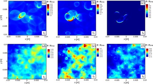
Note that although a few pressure spikes $P_{max}$ reaching $P_{\mathrm{ZND}}$ are observed for Case B, these instantaneous pressure spikes actually stem from the collision and intersection of multiple emerging end-gas autoignition fronts at the late phase of the combustion process. As shown in Figures 4 and 5, the fuel/air mixture is mostly consumed by low-speed ignition fronts, and a negligible amount of the unburned mixture still remains during the end-gas autoignition process that annihilates developing detonation formation, and thus no detonation is observed for Case B.

3.2. Computational singular perturbation (CSP) analysis

Having examined the physical characteristics of pressure and temperature fields, the next step is to examine the dynamics of the system in both cases, in view of the CSP diagnostics and particularly ${\mathrm{\Omega }}_R$, ${\mathrm{\Omega }}_{R+T}$ and ${\mathrm{\Lambda }}_{e,f}$. Recall that ${\mathrm{\Lambda }}_{e,f}$ signifies the regions where an explosive mode is present, with its magnitude being indicative of its timeframe of action, yet without considering the impact of the remaining active modes (dissipative ones) which can potentially have larger impact on the system's slow dynamics. On the other hand, ${\mathrm{\Omega }}_R$ and ${\mathrm{\Omega }}_{R+T}$ are weighted averages of all active (slow) modes (both explosive and dissipative) with weights that depend on their amplitudes. Recall also that ${\mathrm{\Omega }}_R$ and ${\mathrm{\Omega }}_{R+T}$ can take both positive (explosive) and negative (dissipative) values, while ${\mathrm{\Lambda }}_{e,f}$ by definition takes only positive values and indicates explosive dynamics. As a result, ${\mathrm{\Omega }}_R$ and ${\mathrm{\Omega }}_{R+T}$ are defined everywhere in the computational domain, whereas ${\mathrm{\Lambda }}_{e,f}$ only exists in certain parts of the domain. This is confirmed in Figure 6 which shows the spatial distributions of ${\mathrm{\Omega }}_R$, ${\mathrm{\Omega }}_{R+T}$ and ${\mathrm{\Lambda }}_{e,f}$ for both cases at $t_4$, i.e. the instants of the detonation onset for Case 4.

Figure 6. Results for Cases A (a–e) and B (f–j) at $t_4$. From left to right, spatial distributions of ${\mathrm{\Omega }}_R$ (a,f), ${\mathrm{\Omega }}_{R+T}$ (b,g), ${\mathrm{\Lambda }}_{e,f}$ (c,h), ${\mathrm{\Lambda }}_{e,f}$ overlaid with ${\mathrm{\Omega }}_{R+T}>0$ (d,i) and ${\mathrm{\Omega }}_{R+T}$-${\mathrm{\Omega }}_R$ (e,j).

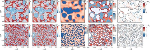
The spatial distributions of ${\mathrm{\Omega }}_R$ and ${\mathrm{\Omega }}_{R+T}$ in both cases in Figure 6(a, b and f, g) show many similarities, but there are regions where ${\mathrm{\Omega }}_R$ and ${\mathrm{\Omega }}_{R+T}$ exhibit significant differences, as shown in Figure 6(e,j). This is where the transport plays a significant role in the system's slow active modes, either positively (shown in red) or negatively (shown in blue). It is seen that positive ${\mathrm{\Omega }}_{R+T}-{\mathrm{\Omega }}_R$ is more pronounced in Case A rather than Case B. In fact, the areas where this difference becomes highly positive in Case A (reaching values as high as 13) are located at the edge of the detonation front where, as it will be confirmed next, transport processes become important.

Second, ${\mathrm{\Lambda }}_{e,f}$ appears to exist in a wider region of the computational domain in contrast to ${\mathrm{\Omega }}_R$ and ${\mathrm{\Omega }}_{R+T}$ which become positive (hence suggesting explosive dynamics) at a much smaller fraction of the computational domain. This clearly indicates a competition between the explosive mode associated with ${\mathrm{\Lambda }}_{e,f}$ and dissipative modes. In the regions where ${\mathrm{\Lambda }}_{e,f}$ exists, but ${\mathrm{\Omega }}_R$ or ${\mathrm{\Omega }}_{R+T}$ are negative, active dissipative modes obtain larger amplitudes than the explosive mode, hence induce a stronger effect on the system's slow evolution. The difference between ${\mathrm{\Lambda }}_{e,f}$ and ${\mathrm{\Omega }}_{R+T}$ is more clearly highlighted in subfigures 6(d) and (i) where the positive ${\mathrm{\Omega }}_{R+T}$ regions (color) are overlaid on positive ${\mathrm{\Lambda }}_{e,f}$ regions (black and white). It is evident that positive ${\mathrm{\Lambda }}_{e,f}$ does not always represent the explosive nature of the system's dynamics, since its action is cancelled by that of more active dissipative mode(s). Only a smaller subset of positive ${\mathrm{\Omega }}_{R+T}$ regions are considered truly explosive. Hence, the diagnostics solely based on ${\mathrm{\Lambda }}_{e,f}$ may lead to an erroneous interpretation of the system's dynamics, since the action of the explosive mode can be cancelled by other dissipative modes, as it was shown in Figure 6), thereby rendering the drawn conclusions, in the best case, questionable [75–81]. This is in agreement with earlier work in turbulent and MILD combustion that reached the same conclusion and highlighted that ${\mathrm{\Lambda }}_{e,f}$ can compete with dissipative modes which become more active (i.e. faster in terms of their timescales and stronger in terms of their amplitudes) [67, 68]. In particular, in Ref. [68] it was reported that turbulent eddies can suppress the system's explosive dynamics in the preheat zone, for premixed turbulent flames at the thin and the distributed reaction zone regimes. In MILD combustion, the differences between ${\mathrm{\Lambda }}_{e,f}$ and ${\mathrm{\Omega }}_{R+T}$ were reported to be even more pronounced [67] and they were attributed to the competition between different chemical pathways. The results presented in Figure 6 corroborate further that the a priori use of solely ${\mathrm{\Lambda }}_{e,f}$ for the characterisation of the system's dynamics is inappropriate.

Another observation from comparing Figures 6 and 4 is that ${\mathrm{\Omega }}_R$, ${\mathrm{\Omega }}_{R+T}$ and ${\mathrm{\Lambda }}_{e,f}$ all become negative (or undefined in the case of ${\mathrm{\Lambda }}_{e,f}$) in the regions where the fuel has been consumed and the temperature is high. However, the converse holds true only for ${\mathrm{\Lambda }}_{e,f}$ but not for ${\mathrm{\Omega }}_R$ and ${\mathrm{\Omega }}_{R+T}$, that is, regions of unburned mixture and low temperature are not always associated with positive values of ${\mathrm{\Omega }}_R$ and ${\mathrm{\Omega }}_{R+T}$. Finally, the energetic length scale of temperature ($l_T$) in Case B directly impacts the spatial distribution of ${\mathrm{\Omega }}_R$, ${\mathrm{\Omega }}_{R+T}$ and ${\mathrm{\Lambda }}_{e,f}$.

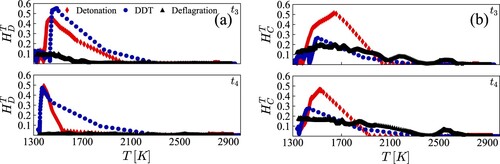
The relation between ${\mathrm{\Omega }}_{R+T}$ and temperature is examined further in Figure 7 which compares the highly positive values of ${\mathrm{\Omega }}_{R+T}$, $4\le {\mathrm{\Omega }}_{R+T}\le 7$, against temperature, 1200 $\le$ T[K] $\le$3000, for both cases at the five selected times in the form of scatter plots. At $t_1$, the two cases exhibit minor differences and reach the same maximum values. At $t_2$, however, a noticeable difference in the maximum ${\mathrm{\Omega }}_{R+T}$ values becomes apparent, with Case A exhibiting higher ${\mathrm{\Omega }}_{R+T}$ values (${\mathrm{\Omega }}_{R+Tmax}=7.3$) than Case B (${\mathrm{\Omega }}_{R+Tmax}=6.8$). At $t_3$, when Case A is just before the knock onset, the difference between the two cases becomes more pronounced and ${\mathrm{\Omega }}_{R+T}$ obtains even higher values than those obtained at $t_2$, and the difference of ${\mathrm{\Omega }}_{R+T}$ between Cases A and B grows to $\sim 10\mathrm{\%}$, with Case A obtaining ${\mathrm{\Omega }}_{R+T}$ values reaching 7.5. At $t_4$, Case A has just passed the detonation onset and the difference in the high ${\mathrm{\Omega }}_{R+T}$ values between the two cases becomes attenuated, decreased to $\sim 2\mathrm{\%}$, with fewer points of Case A obtaining the higher values of $t_3$. Eventually, at $t_5$ the two cases look very similar in terms of their highest ${\mathrm{\Omega }}_{R+T}$ values, ${\mathrm{\Omega }}_{R+Tmax}=7.5$ for both, Case A and Case B.

Figure 7. Scatter plots of ${\mathrm{\Omega }}_{R+T}$ against temperature, for Cases A and B, at the five selected times. For the details of the selected times, see Table 2 and Figure 3.

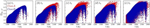
These results indicate that the detonation development is manifested by the highest ${\mathrm{\Omega }}_{R+T}$ mostly prior to the event (i.e. $t_2$, $t_3$) and remains visible immediately after the detonation occurrence at $t_4$. In fact, a careful examination of the data revealed that ${\mathrm{\Omega }}_{R+T}$ in Case A is higher than that in Case B only within the ignition kernels where the detonation develops. This is a significant finding, indicating that the detonation development can be accurately predicted using the appropriate CSP tools. The finding is intuitive because detonation is a result of the positive feedback between the heat release in the ignition front and the pressure wave. The TSR metric serves as an unambiguous marker for the resultant explosive dynamics.

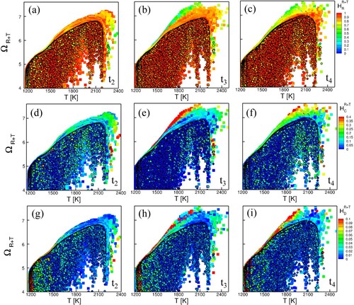
Having identified ${\mathrm{\Omega }}_{R+T}$ as a proper metric to predict detonation, the next question is about the role of transport relative to chemical reactions in driving the explosive dynamics. Figure 8 shows scatter plots of ${\mathrm{\Omega }}_{R+T}$ against temperature as shown in Figure 7, but the data points are coloured according to the TSR-API, i.e. contribution of chemistry (subfigures (a)–(c), convection (d)–(f) and diffusion (g)–(i) for Cases A (square symbols) and B (circle symbols with solid edges), at three selected times ($t_2$-$t_4$). First, the results indicate that chemical reactions indeed play the most important role for both cases at all times. However, note that the data points where ${\mathrm{\Omega }}_{R+T}$ in Case A exceeds that in Case B are characterised by the increased role of transport processes, especially convection. This is manifested at all times but it becomes more pronounced as the detonation onset is approached (at $t_3$), where for Case A $H_C^{R+T}$ reaches values of 0.4, while at the same timestep, $t_3$, the deflagrative system, Case B exhibits $H_C^{R+T}\sim 0.05$. Immediately after the detonation onset, the increased role of the transport processes becomes attenuated. Moreover, the points that extend the explosive dynamics to higher temperatures in Case A are also characterised by the increased role of transport and particularly of convection. On the other hand, the highest contribution of convection is also seen at low and intermediate temperatures (see $t_2$ in Figure 8). Diffusion also appears to have its role increased in the detonating case, but its contribution is relatively small $H_D^{R+T}\le 0.1$ compared to that of convection, $H_C^{R+T}=0.4$.

Figure 8. Scatter plots of ${\mathrm{\Omega }}_{R+T}$ against temperature, for Cases A and B shown with square and circle signs, respectively, at three selected times ($t_2$–$t_4$). Each cell has been coloured based on the contribution of chemical reactions, convection and diffusion, as represented by $H_R^{R+T}$ (a–c), $H_C^{R+T}$ (d–f) and $H_D^{R+T}$ (g–i), respectively. For the details of the selected times, see Table 2 and Figure 3.

All these findings consistently underscore the enhanced role of the transport processes (particularly convection) in the detonation development. However, since Figure 8 shows the entire data points in the computational domain, a subsequent analysis is conducted by confining the observation near the region of the detonation development sites. Figure 9 displays the spatial distributions of pressure and temperature along with the $H_R^{R+T}$, $H_C^{R+T}$ and $H_D^{R+T}$, conditioned to the areas where the dominant dynamics represented by ${\mathrm{\Omega }}_{R+T}$ is explosive (${\mathrm{\Omega }}_{R+T}>0$), in the neighbourhood of the detonation development area, at three different times, $t_2$, $t_3$ and $t_4$.

Figure 9. Pressure, temperature and ${\mathrm{\Omega }}_{R+T}$ fields along with the spatial distributions of $H_R^{R+T}$, $H_C^{R+T}$ and $H_D^{R+T}$, conditioned with ${\mathrm{\Omega }}_{R+T}>0$, for Case A at $t_2$–$t_4$. The analysis focuses on the specific region where the detonation is developed. Dotted black lines are overlaid to mark detonation fronts.

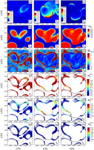
The first notable finding is that the area where pressure reaches high values at $t_3$ and $t_4$ is primarily characterised by dissipative and not explosive dynamics. This is an important point to note, although it may not be surprising considering that the fuel is mostly consumed to yield the high-temperature equilibrium state. In the meantime, the explosive dynamics is observed in the upstream of the periphery of the ignition fronts, with its magnitude decaying over time as the ignition fronts collide and merge.

Second, the explosive dynamics is largely characterised by the enhanced role of chemistry, as evidenced by the high values of $H_R^{R+T}$, predominantly approximating 100%. However, transport processes (primarily convection) appear to have an increased role. In particular, even at the early stage of $t_2$, the locations of explosive dynamics exhibit increased values of $H_C^{R+T}$, which become magnified as time progresses. At $t_3$, some regions of explosive dynamics show the value of $H_C^{R+T}$ exceeding 40%. By comparing with the pressure distribution, it is evident that this area is at the edge of the detonation front. In all cases, except for some small regions as seen in (j), the contribution of diffusive transport, $H_D^{R+T}$, is found to be much smaller, approaching 0% and, in principle, insignificant to the system's slow dynamics. Some very small pockets (both in the physical space as well as in the mixture fraction space, as it will be shown next) where the contribution of diffusion increases to non-negligible values are created due to the local temperature gradients, but these are extremely limited, hence they are deemed insignificant. At $t_4$ after the detonation front is established, while the peak pressure behind the front reaches even higher values, the contribution of convection diminishes, with a decrease of 50% from values of 0.4 to 0.2 in $t_3$ and $t_4$, respectively.

Note that the increased role of the transport processes manifested in Figure 9 (and particularly that of convection, $H_C^{R+T}$) occurs in regions located at the edge of the localised pressure wave. This can be explained by considering that the temporal evolution of the localised pressure waves depends on the onset of ignition kernels which grow in space and eventually collide. The collision and interaction of the multiple ignition kernels (3 in the detonation event displayed in Figure 9) and their associated ignition fronts lead to the increase of the amplitude of the localised pressure waves. Hence, the increased role of transport is highly associated with the augmented amplitude of localised pressure wave, i.e. a stronger pressure wave increases the role of transport that enhances the subsequent detonation development.

This finding is demonstrated both prior to the detonation onset, i.e. at $t_2$ and $t_3$ but also at $t_4$, i.e. when detonation has just started evolving. The established cause-and-effect relationship between detonation onset and the increased role of convection is a unique feature that may be utilised as an important observable for predicting detonation based on the data analysis; the role of convection, conditioned with explosive dynamics along with the ${\mathrm{\Omega }}_{R+T}$, would serve as features for the training of the algorithm. Such a described role of convection in the development of the detonation event is in fact consistent with recent numerical and experimental investigations [82, 83]. Sow et al. [82] reported that convective mixing can be instrumental in the development of detonation structures. In particular, it was reported that gasdynamics due to convective processes could be the controlling mechanism behind jetting phenomena which can lead to complex detonation structures such as shock bifurcations. Shi et al. [83] also recently reported that heat convection (which will be highlighted next in the discussion) is a critical mechanism for detonation extinction in a methane-fuelled system with a water curtain of finite thickness.

To quantify the differences between the detonation development in Case A and the deflagration in Case B, a statistical analysis was performed by computing the averages of ${\mathrm{\Omega }}_R$, ${\mathrm{\Omega }}_{R+T}$, $H_R^{R+T}$, $H_C^{R+T}$ and $H_D^{R+T}$ conditioned against temperature, as the metric to indicate the explosive dynamics, i.e. either ${\mathrm{\Omega }}_R>0$ or ${\mathrm{\Omega }}_{R+T}>0$. For Case A, the statistical average was performed on the regions of detonation development only, as displayed in Figure 9, while for Case B, the entire computational domain was considered for the averaging of ${\mathrm{\Omega }}_R$, ${\mathrm{\Omega }}_{R+T}$, $H_R^{R+T}$, $H_C^{R+T}$ and $H_D^{R+T}$ conditioned against temperature. The results for times $t_2$, $t_3$ and $t_4$ are shown in Figure 10. The rationale for the different averaging procedures between Cases A and B, was to isolate the physical characteristics pertinent to the detonation development, thereby allowing them to stand out in the comparison against non-detonating events (i.e. deflagration and autoignition). Since Case A includes both detonating and non-detonating events, averaging data from the whole domain would smooth out the features associated with the detonating events. It is noted that this comparison is performed with the understanding that Case B contains regions which exhibit prevalent flame propagation and autoignition process (both considered as normal combustion) as opposed to those of Case A which exhibit a dominance of developing detonation process, yet, this approach shall allow extraction of the key features pertinent to detonation. The mixing of the two processes in Case B (deflagration and autoignition) largely explains the non-smooth profile of ${\mathrm{\Omega }}_{R+T}$ in Case B.

Figure 10. (a–c) ${\mathrm{\Omega }}_R$, (d–f) ${\mathrm{\Omega }}_{R+T}$, contributions of (g–i) chemical reactions, (j–l) convection, (m–o) diffusion to ${\mathrm{\Omega }}_{R+T}$, where Case A is denoted with red diamond symbols and for Case B blue triangles are used. The results for Case A are produced on the basis of the computational domain where detonation first develops, i.e. the computational domain illustrated in Figure 9, while for Case B the whole computational domain. In both cases only the points characterised by explosive dynamics were considered (${\mathrm{\Omega }}_R>0$ or ${\mathrm{\Omega }}_{R+T}>0$).

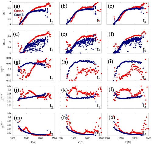
As for the main explosive features, ${\mathrm{\Omega }}_R$ and ${\mathrm{\Omega }}_{R+T}$, Case A exhibits consistently higher level of explosiveness at all times and at medium to high temperatures, 1700< T[K] < 2500, where the detonation front forms. At low to medium temperatures, 1300 < T[K] < 1700, both ${\mathrm{\Omega }}_R$ and ${\mathrm{\Omega }}_{R+T}$ are comparable for Cases A and B. Consistent with the behaviour seen in Figure 7, these findings imply that stronger explosive dynamics associated with detonation is manifested in both ${\mathrm{\Omega }}_R$ and ${\mathrm{\Omega }}_{R+T}$, although the latter exhibits more pronounced difference between Cases A and B. Particularly, from Figure 10(d–f), ${\mathrm{\Omega }}_{R+T}$ of Case B varies between 5.6 and 6.4 at medium to high temperatures, whereas in Case A ${\mathrm{\Omega }}_{R+T}$ reaches values closer to 7 in the same temperature range. This suggests that the inclusion of transport component in predicting explosive dynamics is likely to result in better prediction. Therefore, the training of a ML algorithm in the progress variable space using ${\mathrm{\Omega }}_R$ or ${\mathrm{\Omega }}_{R+T}$ as features and data representative of deflagration combustion mode, would be effective in allowing it to identify points in the physical space that are likely to develop detonation.

Figure 10(g–o) reveals that the explosive dynamics of deflagration, i.e. Case B, is primarily driven by chemical reactions, while for detonation, Case A, the relative contribution of convection increases noticeably, in particular, there is nearly a two-fold difference in $H_C^{R+T}$ between both cases. From (j–l) it is readily obtained that the average convection contribution in Case B yields 6%, while Case A exhibits values reaching $H_C^{R+T}=12\mathrm{\%}$. For all cases at all times, the contributions from the diffusive transport to explosive dynamics remain small.

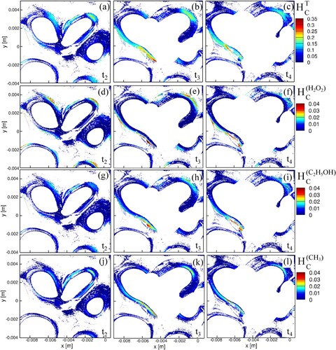
Further analysis of the individual indices revealed that the dominant process responsible for the increase in $H_C^{R+T}$ in the detonating case is heat convection, as illustrated in Figure 11. By comparing Figure 9(j–l) with Figure 11(a–c) it is seen that the regions where $H_C^{R+T}$ obtains high values match those where $H_C^T$ (i.e. the contribution of heat convection) increases significantly. In fact, in these regions $H_C^T$ obtains values of more than 30–35% (in some cases reaching as high as 50%) while the second largest contributor always has a notably smaller contribution that does not exceed 7-8%. As revealed in Figure 11, such contributor can be the convection of CH${}_3$, H${}_2$O${}_2$ or C${}_2$H${}_5$OH (or a combination of these), depending on the region in the physical space. The identification of these species is reasonable since C${}_2$H${}_5$OH is the fuel while CH${}_3$ and H${}_2$O${}_2$ are both radicals participating as reactants in the key reactions associated with the oxidation of ethanol [59]. In particular, H${}_2$O${}_2$ dissociates via a third body chain branching reaction to two OH radicals, H${}_2$O${}_2$ (+M) $\to$ 2OH (+M), while CH${}_3$ facilitates the chain carrying reaction CH${}_3$ + HO${}_2$ $\to$ CH${}_3$O + OH [59]. As a result, the convection of CH${}_3$, H${}_2$O${}_2$ and C${}_2$H${}_5$OH ensures that the reaction front is reinforced, thus, remaining coupled with the shock wave.

Figure 11. The spatial distribution of the contribution of heat convection (a–c) $H_C^T$, and the three highest species' contribution to convection (d–f) $H_C^{(H_2{O}_2)}$, (g–i) $H_C^{(C_2{H}_5\mathrm{OH})}$, (j–l) $H_C^{({\mathrm{CH}}_3)}$, conditioned with ${\mathrm{\Omega }}_{R+T}$ > 0, for Case A at $t_2$ -- $t_4$. The analysis focuses on the specific region where the detonation is developed.

To gain more insight into the interplay between the chemical and transport processes during the transition from deflagration to detonation, one-dimensional (1D) monitor lines normal to the front from Case A were analysed using the CSP/TSR tools. Case A was selected because it exhibits all combustion modes, deflagration, deflagration-to-detonation transition (DDT), and detonation, simultaneously. Three monitor lines were determined, as shown in Figure 12, representing deflagration (line 1), deflagration-to-detonation transition (line 2), and detonation development (line 3). The analysis is particularly focussed on two timesteps, $t_3$ and $t_4$ as these steps sufficiently reveal all three distinct combustion modes.

Figure 12. Spatial distribution of temperature in Case A at two timesteps, $t_3$ and $t_4$. The lines normal to the flame front indicate the 1D monitor lines used for the further CSP/TSR analysis, representing (1) deflagration, (2) deflagration-to-detonation transition (DDT), and (3) detonation.

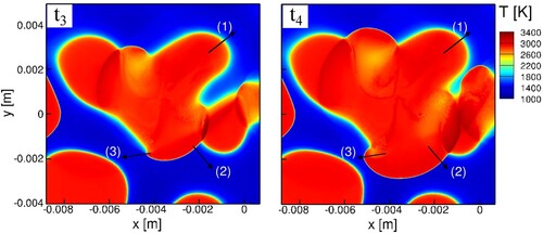
Figure 13 shows the evolution of temperature, normalised pressure (P/$P_{\mathrm{ZND}}$) and mass fraction profiles of C${}_2$H${}_5$OH and OH along the three monitor lines for the two timesteps under study. The pressure profiles indeed confirm the development of detonation for line (3), DDT for line (2) and deflagration for line (1). In all three monitor lines the temperature reaches nearly the same maximum value. The profiles of the mass fractions of C${}_2$H${}_5$OH and OH represent the location of the reaction and flame fronts in the physical space.

Figure 13. Spatial evolution of the normalised pressure (P/$P_{\mathrm{ZND}}$) (a), mass fraction of ethanol (b), temperature (c), mass fraction of OH (d) of the 1D monitor lines displayed in Figure 12 representing deflagration, DDT and detonation at two timesteps, $t_3$ and $t_4$.

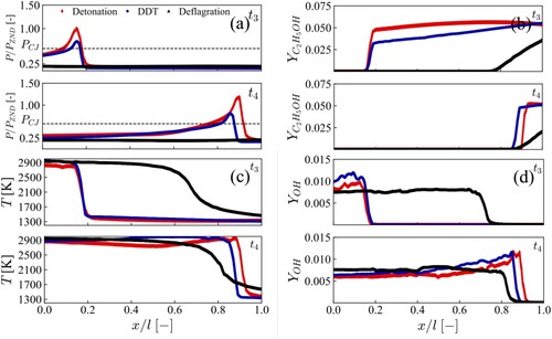
Figure 14 shows the profiles of ${\mathrm{\Omega }}_{R+T}$, ${\mathrm{\Lambda }}_e$, $H_C^{R+T}$, $H_R^{R+T}$ against temperature for the detonation case. The first notable observation is that ${\mathrm{\Omega }}_{R+T}$ becomes negative much earlier (i.e. at much lower temperatures) than ${\mathrm{\Lambda }}_e$. In particular, ${\mathrm{\Omega }}_{R+T}$ turns negative at ∼ 1800 K, while ${\mathrm{\Lambda }}_e$ disappears (i.e. turns negative) at ∼ 2800 K. This suggests that a slow explosive eigenvalue exists within the range of 1800–2800 K, yet its influence on the system's slow dynamics is offset by other slow dissipative modes where the chemistry plays a dominant role, reaching a contribution of 100%. The second important observation is that the region where ${\mathrm{\Omega }}_{R+T}$ is positive, i.e. 1300<T  [K] $<1800$ , is the region typically associated with the flame front. In this region, as the temperature increases, the contribution of chemistry decreases (100% to 10%) while the contributions of both diffusive and convective processes to ${\mathrm{\Omega }}_{R+T}$ increase (40% and 60%, respectively). This contradicts what is typically observed in a flame or autoigniting front, where the contribution of chemistry is significantly enhanced as temperature increases. As will be confirmed later, this is a unique feature of the detonating front. The significantly enhanced role of transport (especially convection) in the region of the explosive dynamics is the result of the coupling between the reaction front and the pressure wave.

Figure 14. CSP/TSR diagnostics against temperature for the 1D monitor line representing the detonation development, displayed in Figure 12, at timestep $t_3$. (a) Evolution of ${\mathrm{\Omega }}_{R+T}$, ${\mathrm{\Lambda }}_e$, $H_R^{R+T}$, $H_C^{R+T}$, $H_D^{R+T}$. (b) Evolution of $H_D^T$, $H_C^T$, the largest contributors to $H_D^{R+T}$, $H_C^{R+T}$, respectively. (c) Evolution of the reactions with the largest contributions to $H_R^{R+T}$.

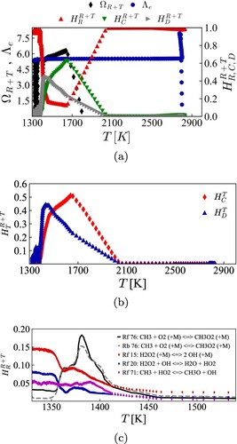
To further examine the transport and reaction processes controlling the explosive dynamics, Figure 14 also shows the (b) diffusive and convective processes with the largest contribution to ${\mathrm{\Omega }}_{R+T}$ as well as (c) the most important reactions. It is evident that the enhanced role of convection is mainly due to convective heat transfer, reaching a maximum contribution of 52% at 1680 K. Heat conduction becomes the largest contributor to the enhanced role of diffusion at 1420 K, reaching a maximum value of 44%. All remaining convective and diffusive processes do not exceed individual contributions of 5% hence their influence is negligibly small. In the region where the contribution of chemistry is important, the most important reaction is initially reaction R15f, H${}_2$O${}_2$(+M)$\to$2OH(+M), which leads to the production of two highly reactive OH radicals. The key role of this reaction to the combustion of ethanol is well documented in the literature (see for example [59]). Reaction R20f, H${}_2$O${}_2$+OH$\to$H${}_2$O+HO${}_2$, competes with R15f in the consumption H${}_2$O${}_2$ hence tends to decrease the influence of the explosive dynamics. Next, there exists a set of three carbon-based reactions which all have in common the CH${}_3$ radical. Reaction R71f, CH${}_3$+HO${}_2\to$CH${}_3$O+OH, competes with R76f, CH${}_3$+O${}_2$(+M)$\to$CH${}_3$O${}_2$(+M), in the depletion of CH${}_3$, but they all lead to key intermediate species in the oxidation of ethanol; CH${}_3$O and OH (R71f) and CH${}_3$O${}_2$ (R76f). Finally, reaction R76b, CH${}_3$+O${}_2$(+M)$\leftarrow$CH${}_3$O${}_2$(+M), balances with R76f. Although the net effect of these two reactions appears to be negligibly small, the role of reaction Rf6 cannot be dismissed as its forward direction promotes explosive dynamics by producing CH${}_3$O${}_2$ while its backward direction opposes by consuming CH${}_3$O${}_2$ and producing the highly reactive methyl radical.

Figures 15 (DDT) and 16 (deflagration) reveal the changes in the structure as the front behaviour shifts from the detonating case to the DDT and then to the deflagration. For example,

• ${\mathrm{\Omega }}_{R+T}$ becomes negative, thereby losing its explosive character at higher temperatures. In particular, in the case of deflagration the explosive dynamics of ${\mathrm{\Omega }}_{R+T}$ is lost at 2100 and 2150  K at $t_3$ and $t_4$, respectively.

• The difference between ${\mathrm{\Lambda }}_{e,f}$ and ${\mathrm{\Omega }}_{R+T}$ is diminished, but remains noticeable. In the deflagration case, ${\mathrm{\Lambda }}_{e,f}$ vanishes at 2210 and 2520  K at $t_3$ and $t_4$, respectively. This suggests a difference of 110 and 370 K for both timesteps, significantly lower than the difference of 1000 K that was observed in the detonating case.

• The contribution of convection to ${\mathrm{\Omega }}_{R+T}$ vanishes. In fact, in the case of deflagration the total contribution of transport never exceeds 30%, i.e. half of the maximum contribution reached by transport in the detonating case.

• Conversely, the contribution of chemistry to ${\mathrm{\Omega }}_{R+T}$ increases and is maintained at a minimum of 65% in the case of deflagration at both timesteps. This also implies that the flame front is controlled by chemistry, in agreement with what has been reported for normal combustion in other setups (e.g. [68])

• The diminishing roles of diffusion and convection are associated with the decreasing contributions of the convective heat transfer and thermal diffusion. In the deflagrating case, the importance of diffusion becomes negligibly small.

Figure 15. Evolution of $H_C^{R+T}$ (a), $H_R^{R+T}$ (b), ${\mathrm{\Omega }}_{R+T}$ (c), ${\mathrm{\Lambda }}_e$ (d) conditioned against temperature, for the 1D monitor lines displayed in Figure 12 representing deflagration, DDT and detonation at two timesteps, $t_3$ and $t_4$.

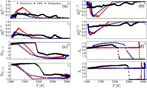
Figure 16. Evolution of $H_D^T$ (a), $H_C^T$ (b) conditioned against temperature, for the 1D monitor lines displayed in Figure 12 representing deflagration, DDT and detonation at two timesteps, $t_3$ and $t_4$.

4. Conclusions

In the present study, two 2D high-fidelity numerical simulations were used as a parametric study to identify key differences in the dynamics of a detonating case against deflagration in view of asymptotic analysis. Advanced mathematical tools developed through the computational singular perturbation framework were used in order to: (i) identify the locations where the dynamics of the system becomes explosive and (ii) investigate the interplay between chemistry and transport processes. The analysis revealed that:

• The detonating case exhibited stronger explosive dynamics, as manifested both in the higher values obtained for the ${\mathrm{\Omega }}_{R+T}$ metric and the wider region in the progress variable space where the dynamics became explosive. This finding suggests a more reactive state obtained for the detonation development.

• The contribution of the chemical reactions was largely the main force driving both the detonation and the deflagration cases.

• In the detonating case, the explosive dynamics was generally characterised by the enhanced role of convection, occurring at the edge of the detonating front.

• The enhanced role of convection in the detonating case was mainly due to heat convection.

• The dynamics of the main part of the detonating front was primarily characterised by dissipative and not explosive dynamics since there the fuel was largely consumed and the temperature was very high.

• The role of diffusion was found to be insignificant in both examined cases.

Disclosure statement

No potential conflict of interest was reported by the author(s).

Additional information

Funding

This work was sponsored by the King Abdullah University of Science and Technology (KAUST) and used the computational resources of the KAUST Supercomputing Laboratory. The authors thank Convergent Science Inc. for providing the CONVERGE license.

Appendix 1.

Validation of CONVERGE CFD against KARFS DNS

The current analysis targets to support the implementation of a low-order numerical method (CONVERGE CFD) in the scope of detonation research, compared to direct numerical simulations, performed by the King Abdullah Univeristy of Science and Technology (KAUST) in-house code, KARFS. The following KARFS DNS simulations are solved from identical initial conditions and imposed temperature inhomogeneity, as prescribed by CONVERGE CFD detonation simulation, Case A.

The figures provided hereby illustrate the strong similarity between the solutions of both CFD codes: CONVERGE CFD and KARFS. Nevertheless, it is important to note that solution approximations and iterative methods contribute to an additive error due to truncation, round-off, consecutively enhancing the effect of numerical diffusion.

A.1. 1D simulations

The presented numerical study considers 1D simulations of stoichiomertic ethanol-air combustion, with a fixed grid cell size of $5\mathrm{mu}\mathrm{m}$ . A temperature map is imposed to emulate the temperature hot spot condition from the 2D simulations presented in the main body. KARFS and CONVERGE CFD codes solve for a 1D flow with the following initial conditions: a Gaussian hot spot of thickness $\sigma =8\mathrm{mm}$, is set with initial conditions $T_{max}=1,150\mathrm{K}$, $T_{min}=1,100\mathrm{K}$, centred at $x=0\mathrm{m}$, with the domain ranging from $-0.02\mathrm{m}$ to $0.02\mathrm{m}$. The initial pressure, $P_{\mathrm{in}}$, is 35 bar.

The computational configuration also accounts for the wall-interaction effect, an important factor in the study of detonation waves, where the pressure wave oscillations promote further the increase of wave strength, resulting in pressure peaks exceeding the Chapman-Jouguet threshold and approaching the von Neumann point. For all cases discussed, the Chapman-Jouguet pressure is computed to be $P_{\mathrm{CJ}}=20\mathrm{MPa}$. Furthermore, the initiation of the detonation mode denoted by the ZND pressure peak is found to be $P_{\mathrm{ZND}}=34.8\mathrm{MPa}$, given in Section 2.1. The species selected to facilitate the comparison are ${\mathrm{C}}_2{\mathrm{H}}_5\mathrm{OH}$, ${\mathrm{CH}}_3$, ${\mathrm{H}}_2{\mathrm{O}}_2$, following the discussion in Section 3.2.

In Figure A2, the temporal evolutions of the maximum temperature hold a strong agreement between the 2 sets of simulations. There exists a difference $\sim 200\mathrm{K}$ or merely 5% between the peak $T_{max}$ values attained by both simulations, while this discrepancy is attenuated at all other times, and is overall negligible.

Figure A1. Imposed initial conditions at $t=0\mathrm{s}$. The blue line represents temperature, while the red line represents fuel mass fraction.

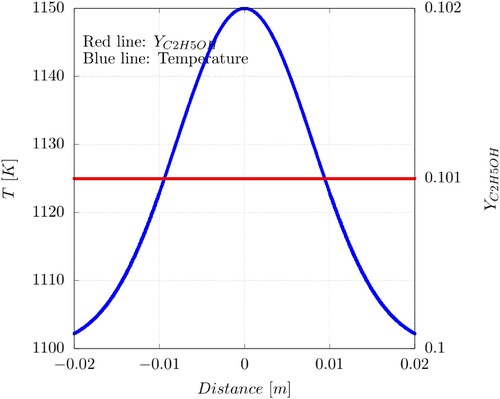
Figure A2. Temporal evolution of $T_{max}$ for 1D CONVERGE CFD and KARFS simulations. The x-axis is normalised by the peak of the normalised pressure.

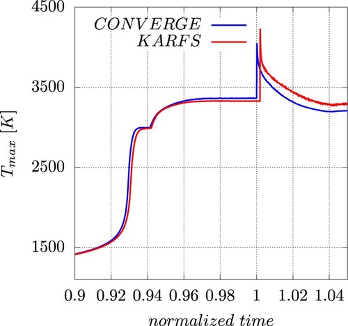
From Figure A3 it becomes apparent that both, KARFS and CONVERGE resolve indeed a detonation front, as opposed to a deflagrative one, supported by maximum pressure values exceeding $P_{\mathrm{ZND}}$, where KARFS DNS simulation yields a stronger detonation wave. Such a discrepancy is simply a direct result of comparing a higher- and a lower-order solver and is intuitive. The comparison is further facilitated with a comparison of different time snapshots, in particular, the three timesteps considered in Figure A4, moving the variables to the physical space. Timestep (1) showcases an early ignition accompanied by relatively low pressures, timestep (2) is characterised by an initiation to the ZND detonation regime by pressure values exceeding $P_{\mathrm{CJ}}=20\mathrm{MPa}$ and approaching $P_{\mathrm{ZND}}$ = 34.8 MPa, and timestep (3) gives an example of a strong wall interaction, oscillations from which the pressure waves intensify further, exceeding $P_{\mathrm{ZND}}$. As seen in Figure A4, the flame propagation in both simulations follows notably similar trends, and the classification of the detonation regime is supported by the pressure values exceeding the von Neumann point in both simulations. It is readily obtained from Figure A4 that at $t_1$ there is a consistent agreement of the pressure profiles. In $t_2$, as the ZND detonation regime is initiated, both simulations exceed $P_{\mathrm{CJ}}$ and approach $P_{\mathrm{ZND}}$, and the difference of the maximum pressure values is under 12%. Once wall interactions become present, the pressure waves successfully exceed $P_{\mathrm{ZND}}$ at the boundaries, at $t_3$.

Figure A3. Temporal evolution of $P_{\mathrm{ZND}}$ for 1D CONVERGE CFD and KARFS simulations. The x-axis is normalised by the peak of the normalised pressure.

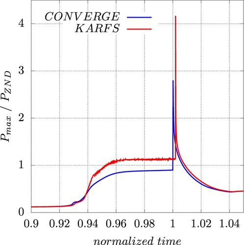
Figure A4. Evolution of pressure and selected species' mass fractions over 3 selected timesteps corresponding to early ignition, detonation onset and peak pressure locations. The blue and red lines highlight the results for CONVERGE CFD and KARFS, respectively. The species' mass fractions $Y_{C2H5\mathrm{OH}}$, $Y_{H2O2}$, $Y_{\mathrm{CH}3}$ are located at rows 2–4.

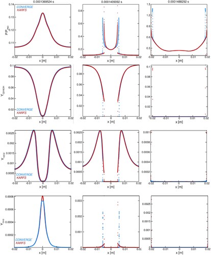
Moreover, the quantitative comparison of the various species' mass fractions confirms a satisfactory convergence of results covered by the 3 selected timesteps, which observation can be extended to any time instant of the systems' evolution. At $t_3$ the species' mass fraction results convey the nearly complete depletion of the species, with insignificant traces of species active at the boundaries, hence the results stated in $t_1$–$t_2$ are of higher interest to the current discussion. In particular, at $t_1$ the profiles of $Y_{C_2{H}_5\mathrm{OH}}$ and $Y_{H_2{O}_2}$ are in perfect agreement between the KARFS and CONVERGE simulations, whereas the profiles of $Y_{C{H}_3}$ follow the same trend, with KARFS yielding $Y_{C{H}_3}=0.00081$, ∼ 12% higher than the peak value of the CONVERGE simulation. At $t_2$, as the detonation waves propagate to the left and right of the origin, $x=0\mathrm{m}$, there is a slight decrease in the accuracy of the comparison between the two simulation sets for the mass fractions of the species. However, the important physical properties remain well preserved.

A.2. 2D simulations

The authors would like to further emphasise the agreement between the two 1D data sets and draw attention to the $2^{\mathrm{nd}}$ portion of the discussion revolving around 2D simulations. A new 2D simulation was performed by KARFS, with identical to Case A initial conditions, the detailed numerical setup is available in Table 1.

The authors want to bring the reader's attention to Figure A5. The temperature contours of the KARFS and CONVERGE simulations have a remarkable similarity, both quantitatively and qualitatively, for timesteps $t_1$–$t_5$. As previously suggested, the Reynolds-averaged Navier-Stokes RANS method used with CONVERGE CFD strikes a good balance between accuracy and computational demands. However, this method does have a smoothing effect on the flame fronts, e.g. comparing the main hotspot profiles in $t_1$–$t_4$ between the two simulation sets. It is clear that KARFS effectively solves the system's dynamics with greater precision, resulting in expected variances in localised flow fields upon comparison with CONVERGE. Similarly, Figure A6 presents snapshots of the temporal range of $t_2$–$t_4$, as per Figure 5 of the evolution of pressure, further emphasising the quantitative and qualitative similarities between the KARFS and CONVERGE simulations. Both sets of simulations accurately retain the nature of the detonation front and its essential physical properties.

Figure A5. Temporal evolution of temperature for the range of $t_1$–$t_5$, as per outlined in the main body. Subfigures (a–e) and (f–j) correspond to the two sets of numerical case studies, CONVERGE CFD software and KARFS DNS, respectively.

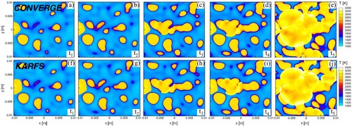
Figure A6. Temporal evolution of the normalised pressure contour ($P_{max}$/$P_{\mathrm{ZND}}$) for the time range $t_3$–$t_5$, complimenting Figure 5.

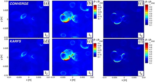
Furthermore, two additional figures are presented, in particular Figures A7 and A8, portraying the temporal evolution of the mean temperature and normalised pressure, respectively. The former presents similar results between the two sets of simulations following consistent trends. The latter, Figure A8, showcases the propensity to detonation for CONVERGE and KARFS simulations, and the normalised $P_{max}$ results for DNS reach values of 9.9, whereas CONVERGE results yield $P_{max}/P_{\mathrm{ZND}}=8.9$ at the peak. The wall interference of the pressure waves and the resonance resulting from it cause the pertinent irregularities in Figure A8 inherent to both, the CONVERGE and KARFS results.

Figure A7. Mean temperature exhibited by CONVERGE CFD (blue solid line) and KARFS (red solid line) in the time range approximating ignition delay.

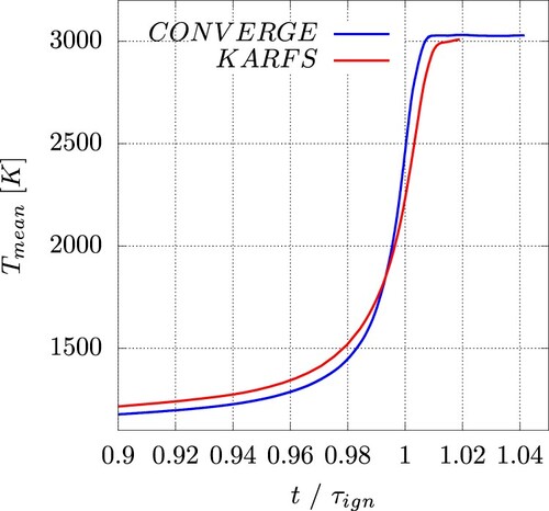
Figure A8. Normalized pressure (P/$P_{\mathrm{ZND}}$) plot denoting detonation propensity in the simulations by CONVERGE CFD (blue solid line) and KARFS (red solid line) in the time range approximating ignition delay.

References

- M.D. Lorenzo, P. Brequigny, F. Foucher, and C. Mounaim-Rousselle, Turbulent flame speed of a gasoline surrogate in conditions representative of modern downsized spark-ignition engine, Combust. Flame. 240 (2022), p. 112041.
- S. Baek, H. Lee, and K. Lee, Fuel efficiency and exhaust characteristics of turbocharged diesel engine equipped with an electric supercharger, Energy 214 (2021), p. 119049.
- X. Zhao, Z. Zhu, Z. Zheng, Z. Yue, H. Wang, and M. Yao, Effects of flame propagation speed on knocking and knock-limited combustion in a downsized spark ignition engine, Fuel 293 (2021), p. 120407.
- Y. Wang, H. Wei, L. Zhou, X. Zhang, and L. Zhong, Effects of reactivity inhomogeneities on knock combustion in a downsized spark-ignition engine, Fuel 278 (2020), p. 118317.
- J.E. Dec, Y. Yang, and N. Dronniou, Improving efficiency and using E10 for higher loads in boosted engines, Sae Int. J. Engines 5 (2012), pp. 1009–1032.
- J.R. Serrano, P. Piqueras, J. De La Morena, A. Gómez-Vilanova, and S. Guilain, Methodological analysis of variable geometry turbine technology impact on the performance of highly downsized spark-ignition engines, Energy 215 (2021), p. 119122.
- M.B. Luong, F.E. Hernández Pérez, and H.G. Im, Prediction of ignition modes of NTC-fuel/air mixtures with temperature and concentration fluctuations, Combust. Flame.213 (2020), pp. 382–393.
- Z. Wang, Y. Qi, X. He, J. Wang, S. Shuai, and C.K. Law, Analysis of pre-ignition to super-knock: Hotspot-induced deflagration to detonation, Fuel 144 (2015), pp. 222–227.
- K. Morganti, M. Abdullah, A. Alzubail, Y. Viollet, R. Head, J. Chang, and G. Kalghatgi, Improving the efficiency of conventional spark-ignition engines using octane-on-demand combustion-part I: Engine studies, SAE Technical Paper 2016–01–0679, 2016.
- G. Kalghatgi, K. Morganti, I. Algunaibet, M. Sarathy, and R. Dibble, Knock prediction using a simple model for ignition delay, Shock 1 (2016), p. 3.
- L. Chen, T. Li, T. Yin, and B. Zheng, A predictive model for knock onset in spark-ignition engines with cooled EGR, Energy Conversion Manage. 87 (2014), pp. 946–955.
- Y. Ze'ldovich, Regime classification of an exothermic reaction with nonuniform initial conditions, Combust. Flame 39 (1980), pp. 211–214.
- J.H.S. Lee, The detonation phenomenon, Cambridge University Press, Cambridge, 2008.
- Z. Wang, H. Liu, and R.D. Reitz, Knocking combustion in spark-ignition engines, Prog. Energy. Combust. Sci. 61 (2017), pp. 78–112.
- Z. Gong, L. Feng, and Z. Wang, Experimental and numerical study of the effect of injection strategy and intake valve lift on super-knock and engine performance in a boosted gdi engine, Fuel 249 (2019), pp. 309–325.
- P. Dai and Z. Chen, Effects of nox addition on autoignition and detonation development in dme/air under engine-relevant conditions, Proc. Combust. Inst. 37 (2019), pp. 4813–4820.
- H. Liu, Z. Wang, Y. Qi, X. He, Y. Wang, and J. Wang, Super-knock suppression for highly turbocharged spark ignition engines using the fuel of propane or methanol, Energy 169 (2019), pp. 1112–1118.
- M.J. Mubarak Ali, F. Hernandez Perez, S. Vedharaj, R. Vallinayagam, R. Dibble, and H. Im, Effect of timing and location of hotspot on super knock during pre-ignition, SAE Technical Paper 2017–01–0686, 2017.
- P. Dai, Z. Chen, X. Gan, and M.A. Liberman, Autoignition and detonation development from a hot spot inside a closed chamber: Effects of end wall reflection, Proc. Combust. Inst. 38 (2021), pp. 5905–5913.
- D. Bradley, C. Morley, X.J. Gu, and D.R. Emerson, Amplified pressure waves during autoignition: Relevance to cai engines, SAE Trans. 111 (2002), pp. 2679–2690.
- D. Bradley and G. Kalghatgi, Influence of autoignition delay time characteristics of different fuels on pressure waves and knock in reciprocating engines, Combust. Flame. 156 (2009), pp. 2307–2318.
- Gautam T Kalghatgi and Derek Bradley, Pre-ignition and ‘super-knock’ in turbo-charged spark-ignition engines, Int. J. Engine Res. 13 (2012), pp. 399–414.
- C. Qi, P. Dai, H. Yu, and Z. Chen, Different modes of reaction front propagation in n-heptane/air mixture with concentration non-uniformity, Proc. Combust. Inst. 36 (2017), pp. 3633–3641.
- J. Su, P. Dai, and Z. Chen, Detonation development from a hot spot in methane/air mixtures: Effects of kinetic models, Int. J. Engine Res. 22(8) (2020), p. 146808742094461.
- Y. Gao, P. Dai, and Z. Chen, Numerical studies on autoignition and detonation development from a hot spot in hydrogen/air mixtures, Combust. Theory Modell. 24 (2020), pp. 245–261.
- A. Sow, B.J. Lee, F.E. Hernández Pérez, and H.G. Im, Detonation onset in a thermally stratified constant volume reactor, Proc. Combust. Inst. 37 (2019), pp. 3529–3536.
- M.B. Luong and H.G. Im, Prediction of the developing detonation in an ntc-fuel/air mixture with temperature inhomogeneities under engine conditions, Proc. Combust. Inst. 39 (2023), pp. 4979–4988.
- N. Peters, B. Kerschgens, and G. Paczko, Super-knock prediction using a refined theory of turbulence, Sae Int. J. Engines 6 (2013), pp. 953–967.
- J. Rudloff, J.M. Zaccardi, S. Richard, and J.M. Anderlohr, Analysis of pre-ignition in highly charged SI engines: Emphasis on the auto-ignition mode, Proc. Combust. Inst. 34 (2013), pp. 2959–2967.
- M.B. Luong and H.G. Im, Prediction of ignition modes in shock tubes relevant to engine conditions, in Engines and Fuels for Future Transport, Springer, Singapore, 2022, pp. 369–393. https://doi.org/10.1007/978-981-16-8717-4_15
- M. Figueroa-Labastida, M.B. Luong, J. Badra, H.G. Im, and A. Farooq, Experimental and computational studies of methanol and ethanolpreignition behind reflected shock waves, Combust. Flame 234 (2021), p. 111621.
- F. Takens, Partially hyperbolic fixed points, Topology 10 (1971), pp. 133–147.
- S.H. Lam and D.A. Goussis, Understanding complex chemical kinetics with computational singular perturbation, in Symposium (International) on Combustion, Vol. 22, Elsevier, 1989, pp. 931–941. https://doi.org/10.1016/S0082-0784(89)80102-X
- S.H. Lam and D. Coussis, Conventional asymptotics and computational singular perturbation for simplified kinetics modelling, in Reduced Kinetic Mechanisms and Asymptotic Approximations for Methane-Air Flames, Springer, Berlin, 2005, pp. 227–242. https://doi.org/10.1007/BFb0035372
- M. Hadjinicolaou and D.A. Goussis, Asymptotic solution of stiff pdes with the csp method: The reaction diffusion equation, SIAM. J. Sci. Comput. 20 (1998), pp. 781–810.
- J. Prager, H.N. Najm, M. Valorani, and D. Goussis, Structure of n-heptane/air triple flames in partially-premixed mixing layers, Combust. Flame. 158 (2011), pp. 2128–2144.
- D.G. Patsatzis and D.A. Goussis, A new michaelis-menten equation valid everywhere multi-scale dynamics prevails, Math. Biosci. 315 (2019), p. 108220.
- D.G. Patsatzis, D.T. Maris, and D.A. Goussis, Asymptotic analysis of a target-mediated drug disposition model: Algorithmic and traditional approaches, Bull. Math. Biol. 78 (2016), pp. 1121–1161.
- K.J. Richards, P.K. Senecal, and E. Pomraning, Converge 3.0.13, Convergent Science, Madison, WI, 2023.
- F.E.H. PÉRez, N. Mukhadiyev, X. Xu, A. Sow, B.J. Lee, R. Sankaran, and H.G. Im, Direct numerical simulations of reacting flows with detailed chemistry using many-core/gpu acceleration, Comput. Fluids. 173 (2018), pp. 73–79.
- S. Desai, Y.J. Kim, W. Song, M.B. Luong, F.E.H. PÉRez, R. Sankaran, and H.G. Im, Direct numerical simulations of turbulent reacting flows with shock waves and stiff chemistry using many-core/GPU acceleration, Comput. Fluids. 215 (2021), p. 104787.
- M. Jaasim, E.A. Tingas, F.E.H. PÉRez, and H.G. Im, Computational singular perturbation analysis of super-knock in SI engines, Fuel 225 (2018), pp. 184–191.
- C. Netzer, L. Seidel, M. Pasternak, H. Lehtiniemi, C. Perlman, F. Ravet, and F. Mauss, Three-dimensional computational fluid dynamics engine knock prediction and evaluation based on detailed chemistry and detonation theory, Int. J. Engine Res. 19 (2018), pp. 33–44.
- P. Pal, S. Demir, P. Kundu, and S. Som, Large-eddy simulations of methane-oxygen combustion in a rotating detonation rocket engine, in AIAA Propulsion and Energy 2021 Forum, 2021, p. 3642. https://doi.org/10.2514/6.2021-3642
- N.O. Attal and G. Kumar, Deflagration to detonation transition in two-dimensional obstructed channels, in AIAA Scitech 2022 Forum, AIAA SCITECH 2022 Forum, San Diego, CA, 2022, p. 0392. https://doi.org/10.2514/6.2022-0392
- P.K. Senecal, E. Pomraning, K.J. Richards, T.E. Briggs, C.Y. Choi, R.M. Mcdavid, and M.A. Patterson, Multi-dimensional modeling of direct-injection diesel spray liquid length and flame lift-off length using CFD and parallel detailed chemistry, SAE Technical Paper 2003–01–1043, 2003.
- M.B. Luong, S. Desai, F.E.H. PÉRez, R. Sankaran, B. Johansson, and H.G. Im, A statistical analysis of developing knock intensity in a mixture with temperature inhomogeneities, Proc. Combust. Inst. 38 (2021), pp. 5781–5789.
- M.B. Luong, S. Desai, F.E. HernÁndez PÉrez, R. Sankaran, B. Johansson, and H.G. Im, Effects of turbulence and temperature fluctuations on knock development in an ethanol/air mixture, Flow Turbul. Combust 106 (2021), pp. 575–595.
- A. Bhagatwala, J.H. Chen, and T. Lu, Direct numerical simulations of Hcci/Saci with ethanol, Combust. Flame. 161 (2014), pp. 1826–1841.
- M.B. Luong and H.G. Im, Effects of low-temperature chemistry on direct detonation initiation by a hot spot under engine conditions, Proc. Combust. Inst. 39 (2023), pp. 4989–4999.
- M. Frenklach, Modeling, in Combustion Chemistry, W.C. Gardiner, ed., Springer, New York, NY, 1984, pp. 423–453.
- S. Vajda, P. Valko, and T. Turanyi, Principal component analysis of kinetic models, Int. J. Chem. Kinet. 17 (1985), pp. 55–81.
- J.C. Sutherland and A. Parente, Combustion modeling using principal component analysis, Proc. Combust. Inst. 32 (2009), pp. 1563–1570.
- M. Valorani, S. Paolucci, E. Martelli, T. Grenga, and P.P. Ciottoli, Dynamical system analysis of ignition phenomena using the tangential stretching rate concept, Combust. Flame. 162 (2015), pp. 2963–2990.
- M. Valorani, P.P. Ciottoli, and R.M. Galassi, Tangential stretching rate (TSR) analysis of non premixed reactive flows, Proc. Combust. Inst. 36 (2017), pp. 1357–1367.
- D.A. Goussis, H.G. Im, H.N. Najm, S. Paolucci, and M. Valorani, The origin of cema and its relation to csp, Combust. Flame. 227 (2021), pp. 396–401.
- M. Valorani, F. Creta, P.P. Ciottoli, R. Malpica Galassi, D. Goussis, H. Najm, S. Paolucci, H.G. Im, E.A. Tingas, D. Manias, A. Parente, Z. Li, and T. Grenga, Computational singular perturbation method and tangential stretching rate analysis of large scale simulations of reactive flows: Feature tracking, time scale characterization, and cause/effect identification. Part 1, Basic concepts, in Data Analysis for Direct Numerical Simulations of Turbulent Combustion, Springer, Cham, 2020, pp. 43–64. https://doi.org/10.1007/978-3-030-44718-2_3
- M. Valorani, F. Creta, P.P. Ciottoli, R. Malpica Galassi, D. Goussis, H. Najm, S. Paolucci, H.G. Im, E.A. Tingas, D. Manias, A. Parente, Z. Li, and T. Grenga, Computational singular perturbation method and tangential stretching rate analysis of large scale simulations of reactive flows: Feature tracking, time scale characterization, and cause/effect identification. Part 2, Analyses of ignition systems, laminar and turbulent flames, in Data Analysis for Direct Numerical Simulations of Turbulent Combustion, Springer, Cham, 2020, pp. 65–88. https://doi.org/10.1007/978-3-030-44718-2_4
- E.A. Tingas, D.C. Kyritsis, and D.A. Goussis, Autoignition dynamics of dme/air and etoh/air homogeneous mixtures, Combust. Flame. 162 (2015), pp. 3263–3276.
- E.A. Tingas, The chemical dynamics of hydrogen/hydrogen peroxide blends diluted with steam at compression ignition relevant conditions, Fuel 296 (2021), p. 120594.
- K.K. Yalamanchi, E.A. Tingas, H.G. Im, and S.M. Sarathy, Screening gas-phase chemical kinetic models: Collision limit compliance and ultrafast timescales, Int. J. Chem. Kinet. 52 (2020), pp. 599–610.
- E.A. Tingas, D.C. Kyritsis, and D.A. Goussis, H 2/air autoignition dynamics around the third explosion limit, J. Energy Eng. 145 (2019), p. 04018074.
- D.A. Goussis and M. Valorani, The appropriate context for the analysis of the explosive mode in reactive systems, J. Energy Eng. 149 (2023), p. 04023039.
- H.N. Najm, M. Valorani, D.A. Goussis, and J. Prager, Analysis of methane–air edge flame structure, Combust. Theory Modell. 14 (2010), pp. 257–294.
- E.A. Tingas, Computational analysis of the effect of hydrogen peroxide addition on premixed laminar hydrogen/air flames, Fuel 302 (2021), p. 121081.
- W. Song, E.A. Tingas, and H.G. Im, A computational analysis of methanol autoignition enhancement by dimethyl ether addition in a counterflow mixing layer, Combust. Flame.195 (2018), pp. 84–98.
- D.M. Manias, E.A. Tingas, Y. Minamoto, and H.G. Im, Topological and chemical characteristics of turbulent flames at mild conditions, Combust. Flame. 208 (2019), pp. 86–98.
- D.M. Manias, E.A. Tingas, F.E.H. PÉRez, R.M. Galassi, P.P. Ciottoli, M. Valorani, and H.G. Im, Investigation of the turbulent flame structure and topology at different Karlovitz numbers using the tangential stretching rate index, Combust. Flame. 200 (2019), pp. 155–167.
- M. Valorani, F. Creta, and D.A. Goussis, Local and global manifolds in stiff reaction-diffusion systems, in Computational Fluid and Solid Mechanics 2003, Elsevier, 2003, pp. 1548–1551. https://doi.org/10.1016/B978-008044046-0.50378-X
- D.A. Goussis, M. Valorani, F. Creta, and H.N. Najm, Reactive and reactive-diffusive time scales in stiff reaction-diffusion systems, Progress Comput. Fluid Dyn., Int. J. 5 (2005), pp. 316–326.
- M. Valorani, H.N. Najm, and D.A. Goussis, Csp analysis of a transient flame-vortex interaction: Time scales and manifolds, Combust. Flame. 134 (2003), pp. 35–53.
- R.M. Galassi, Pycsp: A python package for the analysis and simplification of chemically reacting systems based on computational singular perturbation, Comput. Phys. Commun. 276 (2022), p. 108364.
- C. Safta, H.N. Najm, and O. Knio, Tchem-a software toolkit for the analysis of complex kinetic models, Tech. Rep., Sandia National Lab.(SNL-CA), Livermore, CA (USA), 2011.
- Z. Wang, H. Liu, T. Song, Y. Qi, X. He, S. Shuai, and J. Wang, Relationship between super-knock and pre-ignition, Int. J. Engine Res. 16 (2015), pp. 166–180.
- S. Farjam and B. Savard, Ignition and flame stabilization of n-dodecane turbulent premixed flames under spray a thermochemical conditions, Combust. Flame. 242 (2022), p. 112133.
- Z. Huang, M.J. Cleary, Z. Ren, and H. Zhang, Large eddy simulation of a supersonic lifted hydrogen flame with sparse-Lagrangian multiple mapping conditioning approach, Combust. Flame. 238 (2022), p. 111756.
- J.H. Kim, G.H. Yu, S.H. Chung, and C.S. Yoo, A DNS study of ignition characteristics of a lean PRF/air mixture with CH 2O and H 2O 2 addition under HCCI combustion-relevant conditions, Combust. Flame. 234 (2021), p. 111654.
- Z. Zhang, A. Abdelsamie, C. Chi, D. Thevenin, and K.H. Luo, Combustion mode and mixing characteristics of a reacting jet in crossflow, Energy. Fuels. 35 (2021), pp. 13325–13337.
- H. Wang, Z. Wang, K. Luo, E.R. Hawkes, J.H. Chen, and J. Fan, Direct numerical simulation of turbulent boundary layer premixed combustion under auto-ignitive conditions, Combust. Flame. 228 (2021), pp. 292–301.
- M. Zhao, Z. Ren, and H. Zhang, Pulsating detonative combustion in n-heptane/air mixtures under off-stoichiometric conditions, Combust. Flame. 226 (2021), pp. 285–301.
- A. Krisman, P. Meagher, X. Zhao, J.W. Park, T. Lu, and J.H. Chen, A direct numerical simulation of jet a flame kernel quenching, Combust. Flame. 225 (2021), pp. 349–363.
- A. Sow, S.M. Lau-Chapdelaine, and M. Radulescu, The effect of the polytropic index γ on the structure of gaseous detonations, Proc. Combust. Inst. 38 (2021), pp. 3633–3640.
- J. Shi, Y. Xu, W. Ren, and H. Zhang, Critical condition and transient evolution of methane detonation extinction by fine water droplet curtains, Fuel 315 (2022), p. 123133.