ESP: a tool to estimate scale parameter for multiresolution image segmentation of remotely sensed data

Abstract

The spatial resolution of imaging sensors has increased dramatically in recent years, and so too have the challenges associated with extracting meaningful information from their data products. Object-based image analysis (OBIA) is gaining rapid popularity in remote sensing science as a means of bridging very high spatial resolution (VHSR) imagery and GIS. Multiscalar image segmentation is a fundamental step in OBIA, yet there is currently no tool available to objectively guide the selection of appropriate scales for segmentation. We present a technique for estimating the scale parameter in image segmentation of remotely sensed data with Definiens Developer®. The degree of heterogeneity within an image-object is controlled by a subjective measure called the ‘scale parameter’, as implemented in the mentioned software. We propose a tool, called estimation of scale parameter (ESP), that builds on the idea of local variance (LV) of object heterogeneity within a scene. The ESP tool iteratively generates image-objects at multiple scale levels in a bottom-up approach and calculates the LV for each scale. Variation in heterogeneity is explored by evaluating LV plotted against the corresponding scale. The thresholds in rates of change of LV (ROC-LV) indicate the scale levels at which the image can be segmented in the most appropriate manner, relative to the data properties at the scene level. Our tests on different types of imagery indicated fast processing times and accurate results. The simple yet robust ESP tool enables fast and objective parametrization when performing image segmentation and holds great potential for OBIA applications.

Keywords:

• local variance
• OBIA
• tessellation
• characteristic scales
• Definiens

1. Introduction

Traditional pixel-based image classification approaches are poorly suited to very high spatial resolution (VHSR) imagery because within-class spectral variation increases with increased spatial resolution (Schiewe et al. 2001, Aplin 2006). Object-based image analysis (OBIA) arose through the realization that image-objects hold more real-world value than pixels alone (Fisher 1997, Blaschke and Strobl 2001, Smith et al. 2007). Representation of the world in terms of discrete objects better satisfies human understanding (Goodchild et al. 2007). The first and most critical step in OBIA is the creation of image-objects through the aggregation of pixels by image segmentation. Segmentation is the process of dividing remotely sensed images into discrete regions or objects that are homogeneous with regard to spatial or spectral characteristics (Ryherd and Woodcock 1996). The segmentation process reduces the within-class spectral variation of VHR imagery, and can increase the classification and statistical accuracy if conducted at an appropriate scale (Blaschke 2003, Addink et al. 2007).

Defining the most suitable scale for image segmentation is problematic, however, as no objective method currently exists for setting the scale parameter in segmentation algorithms (Kim et al. 2008). Despite the fact that OBIA is becoming increasingly prominent in remote sensing science (Blaschke et al. 2008), the selection of segmentation scale parameters is often dependent on subjective trial-and-error methods (Meinel and Neubert 2004). As Hay et al. (2005) pointed out, ‘the real challenge is to define appropriate segmentation parameters (typically based on spectral homogeneity, size, or both) for the varying sized, shaped, and spatially distributed image-objects composing a scene, so that segments can be generated that satisfy user requirements.’ (p. 341).

The challenges of linking scale to the intrinsic spatial attributes of images are not new in remote sensing science (Marceau and Hay 1999). Based on previous work of Strahler et al. (1986), a groundbreaking concept in this area was introduced by Woodcock and Strahler (1987), who used local variance (LV) graphs to reveal the spatial structure of images. This idea was later introduced in the context of OBIA by Kim et al. (2008). In parallel, a suite of papers (Hay et al. 1997, Hall et al. 2004, Hay et al. 2005) developed this approach further. However, a ready-to-use application allowing the user to evaluate the scale parameter as a function of the intrinsic spatial structure of images is still missing in OBIA.

We carry the concept of LV further and present an automated tool that we have developed to objectively identify the most suitable range of scale parameters at which to conduct image segmentation within the Definiens Developer® software suite. In this article, we test the suitability of the estimation of scale parameter (ESP) tool for defining meaningful segmentation scale parameters across a range of different image types and landscapes. The tool we present here answers the requirements for ‘more automated procedures of segmentation for the extraction of high quality features from very high resolution digital images’ (Kim et al. 2008, p. 300).

2. Local variance and multiscale representation in object-based image analysis

The method builds upon Woodcock and Strahler's (1987) fundamental idea of the relationship between spatial structure of images, size of the objects in the real world (or scene following the terminology used by authors), and pixel resolution. The key to matching real-world objects when analyzing their model (image) is finding the appropriate pixel resolution. The cited authors proposed measuring LV as the value of standard deviation (SD) in a small neighborhood (3 × 3 moving window), then computing the mean of these values over the entire image. The obtained value is an indicator of the local variability in the image. The procedure is applied on successively coarser scales, achieved through resampling techniques. Graphs of values across scales are used to measure spatial structure in images. The authors explain the mechanism as follows: ‘If the spatial resolution is considerably finer than the objects in the scene, most of the measurements in the image will be highly correlated with their neighbors and a measure of local variance will be low. If the objects approximate the size of the resolution cells, then the likelihood of neighbors being similar decreases and the local variance rises’ (p. 313). Basically, the application of LV concept exploits spatial autocorrelation, which is a fundamental image characteristic (Lees 2006).

Kim et al. (2008) made advances toward addressing this issue in the context of OBIA by exploring the relationship between segment variance and spatial autocorrelation at different scale parameters to define the optimal object size. Instead of calculating SD from a 3 × 3 moving window, however, they derived it from objects obtained through segmentation. Their results are particularly important for understanding how changes in the spatial structure of images across scales can be evaluated as a function of LV, spatial autocorrelation, and the number of objects.

The above methods focused on one optimal scale, which is appropriate for simple scene models (cf. Strahler et al. 1986). Because many environmental problems cannot be handled at a single scale of observation (Marceau 1999, Silván-Cárdenas et al. 2009), researchers often have to deal with nested models of a scene (Strahler et al. 1986, Woodcock and Strahler 1987). As such, multiscale analysis and representation require more than one suitable scale parameter to account for different levels of organization in landscape structure. The same applies to complex scenes, particularly when they include different categories of objects with different sizes. Therefore, we extend the concept of LV into multiscale analysis.

The hypothesis underpinning our method is as follows: When growing the size of a segment, its SD increases continuously, up to the point that it matches the object in the real world. Assuming a certain amount of spectral contrast between the object and background, the object boundaries will be preserved in segmentation at a number of higher levels, where the SD of this object remains the same. In the same way, objects of similar size and spectral response are expected to match their correspondents in the real world around the same scale level. As such, their boundaries, and implicitly their SD values, will be conserved along a number of further coarser scale levels. If this type of object is well represented in the image, the cumulative effect of preserving the SD values of objects right above the meaningful scale level will be strong enough to impact upon the LV of that image. On a graph, the LV curve would flatten out, thus pointing to a scale-level representative for that type of object.

Similarly, supposing the object is part of a larger one (e.g., a tree as part of a forest stand), increasing the scale parameter will also lead to an increase in SD, until the segment matches its correspondent at a higher level of organization (i.e., the forest stand), above which SD stagnates again and LV changes. This process repeats as a function of both scene complexity (e.g., variety in object categories) and number of levels in which its objects are organized.

When plotting LV against scale parameter values, we expect to obtain an ascendant graph, with break points indicating optimal scale parameters, at which segmentation produces meaningful levels (e.g., levels of image-objects delineated as they are organized within the scene).

3. Methods

The ESP tool allows for a fast estimation of scale parameters for a multiresolution segmentation in the Definiens® software environment. The ESP tool automatically segments the user-defined data with fixed increments of scale parameter, and calculates LV as the mean SD of the objects for each object level obtained through segmentation. Graphics of LV are used to evaluate the appropriate scale parameters, relative to data properties of the scene.

Multiresolution segmentation in the Definiens® software is a bottom-up region-merging technique starting with one-pixel objects. In numerous iterative steps, smaller image-objects are merged into larger ones. The objects created following this stepwise approach undergo an optimization process, which tries to minimize the internal weighted heterogeneity of each object. Thus, for each object the smallest possible growth is calculated. If the object properties exceed the heterogeneity threshold, defined by the scale parameter, the growth of this object stops (local optimization procedure; Benz et al. 2004). Heterogeneity is defined in terms of the color (spectral values of the pixels forming the object) and shape of the object. These factors can be interactively weighted by the user: the higher the shape factor is weighted, the lower the influence of color values in the segmentation, and vice versa. For the shape factor, it is also necessary to calibrate a compactness and smoothness value influencing the object generation. If compactness is weighted low, the smoothness factor is increased and objects with a more linear shape are favored in the weighting of heterogeneity. On the contrary, higher compactness values will result in more compact objects. In short, a higher scale parameter leads to larger and less homogeneous objects by increasing the threshold of heterogeneity per object. But it is important to note that the scale parameter not be straightforwardly linked to a certain object size. This makes it very difficult to find an appropriate value of scale parameter without performing some ‘trial-and-error’ attempts.

The ESP tool is programmed in Cognition Network Language (CNL) in the Definiens Developer® software, a modular programming language for OBIA applications (Tiede and Hoffmann 2006). It is implemented as a customized process to be applied easily like other processes in object-based rule set creation in the Definiens® software (Figure 1). Six user-defined parameters are adjustable: (1) step size of the increasing scale parameter, (2) starting scale parameter for the analysis, (3) the use of an object hierarchy during segmentation, (4) number of loops (i.e., number of scales to be tested), (5) shape weighting, and (6) compactness weighting. Parameters (2), (5), and (6) are used as implemented in the multiresolution segmentation and described by Baatz and Schäpe (2000) and Benz et al. (2004). The tool can be used for analysis of a single layer of image data or other continuous data (e.g., digital surface models).

Figure 1. Screenshot of the estimation of scale parameter tool, implemented as process in the Definiens Developer® software.

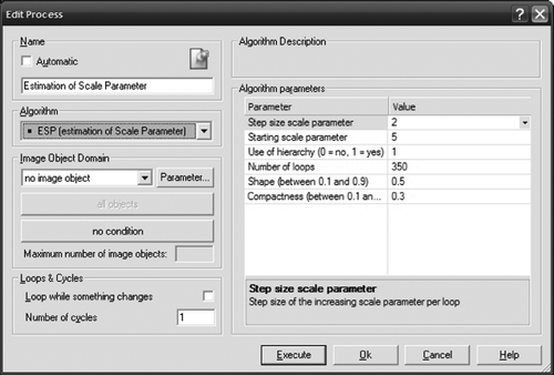
Consideration of hierarchy for image segmentation is of particular importance. If no hierarchy is selected, each segmentation level will be created from scratch. When using the hierarchy option in the ESP tool, each level except for the first one will be based on the previous segmentation. Because the OBIA concept in the Definiens® software uses a strict object hierarchy (i.e., object boundaries of coarser levels are existent in all finer scales), it influences the segmentation process. Therefore, users should carefully decide between using either a multiscale segmentation (MSS) (Burnett and Blaschke 2003) or a one-level representation (OLR) approach (Lang and Langanke 2006), in order to use the tool appropriately.

The results are exported as text files and can be analyzed in any standard spreadsheet application.

To assess the dynamics of LV from an object level to another, we use a measure called rate of change (ROC):

where L = LV at target level and L − 1 = LV at next lower level.

The rate of change is a technical indicator used in stock market analyses to measure ‘the amount of stock's price [that] has changed over a given number of past periods’ (Bauer and Dahlquist 1998, p. 144). This indicator should not be confused with the commonly used receiver operating characteristic (ROC). To avoid this possible confusion, we further refer to rate of change of local variance as ROC-LV. In its original application, this indicator measures changes in time, where ROC-LV measures the amount of change in LV from one object level to another.

We created a spreadsheet template for Excel, where ROC-LV is automatically calculated and plotted.

We hypothesize that peaks in the ROC-LV graph will indicate the object levels at which the image can be segmented in the most appropriate manner, relative to data properties at the scene level. At these peaks, the segments match the types of objects characterized by (relatively) equal degrees of homogeneity. This approach is likely to hold for any type of image-derived objects provided these objects are representative enough to impact on the ROC-LV at the scene level.

We tested the tool on a variety of image types and landscapes (Table 1). Sites were chosen to incorporate a diverse array of scene complexities for exploring the general applicability of the tool. We used familiar data and sites to maximize our expertise in the visual assessment of results. In the first test area (A in Table 1), object types (as represented through their heights in the digital surface model) ranged from individual buildings to blocks of buildings, and from trees to forest stands. In the riparian zone in savanna, objects (as represented on the red channel of a color aerial photograph) are structured in trees and shrubs (continuous transition from individual to stands), with bare soil or grass as background. In the temporary human settlement area, objects are structured in traditional huts and tents, different in size and spectral properties, with a heterogeneous background.

Table 1. Summary of the three test areas and imagery types

Site	Imagery	Resolution	Channel	Landscape	Location
A	LiDAR	1 m	Digital surface model (DSM)	Mixed residential/forest	Austria. North of Salzburg near the village of Bürmoos.
B	Color aerial photography	0.25 m	Red	Riparian zone in savanna landscape	South Africa. Bububu River in the Kruger National Park.
C	QuickBird (pan sharpened)	0.6 m	NIR	Temporary human settlement	Sudan. Zam Zam internally displaced people camp in Dafur.

4. Results

ESP processing times ranged from 1 to 3 min under the ‘hierarchical’ setting and 13–70 min for the ‘nonhierarchical’ option on 1000 × 1000- to 1500 × 1500-pixel subsets of the three test areas (2.5 GHz dual core processor, 4 GB RAM).

4.1. LV and ROC-LV graphs

Both the hierarchical and nonhierarchical options yielded similar results: while LV increased abruptly with increasing segment size at the finer scale parameters, ROC-LV followed an opposite trend (Figure 2). This pattern reveals the transition from pixels to the smallest characteristic objects in scenes of interest. The graphs show that LV alone does not indicate at which scale meaningful objects emerge. However, ROC-LV enhances visualization of these thresholds. We define a threshold as the first break in ROC-LV curve after continuous and abrupt decay. Such a threshold can appear as a step (Figure 2a and b) or as a small peak (Figure 2c).

Figure 2. ESP tool outputs for the three study sites: (a) mixed residential/forested (nonhierarchical), (b) savanna riparian zone (hierarchical), and (c) temporary human settlement (nonhierarchical). Graphs depict changes in local variance (LV) (solid black) and rate of change (ROC) (solid gray) with increasing scale parameter. Dotted vertical lines indicate optimal scale parameters selected for each scene.

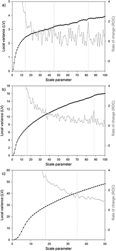
Because of the huge differences in ROC-LV values at the finest scales, variations in ROC-LV curves at coarser scales were obscured. To visually disclose them, vertical axes were rescaled to values just above the first identifiable threshold. All ROC-LV graphs (Figure 2) show sudden oscillations between peaks and plunges, on descendant trends, whereas LV graphs are far smoother. Theoretically, the peaks in an ROC-LV curve indicate the levels where LV increases as segments delineate their correspondents in the real world. However, the variation induced by segmentation of the background also generates peaks, thereby complicating the interpretation of graphs, proportionally to the complexity of scenes. The least complex scene, dominated by two categories of objects (Figure 2c), clearly indicates two peaks (first one corresponding to the threshold as mentioned above), whereas the most complex scene (Figure 2a) shows a much more challenging graph. We selected the most obvious peaks, which dominate their neighborhood, together with the first thresholds in graphs, as indicators for optimal scale parameters (Figure 2).

4.2. Segmentation results

For all images, we selected the peaks as marked in Figure 2 and performed segmentation using the correspondent scale parameters. A visual assessment of these three sites (3–6) shows that the ESP tool accurately identified the suitable scale parameters for segmentation, which delineated meaningful objects that were representative of the various levels of organization within the scenes of interest.

Figure 3. Mixed residential/forested test area: The entire image as segmented and the subset used for visualizing the results (a). Segmentation results with scale parameters of 14 (b), 45 (c), and 82 (d).

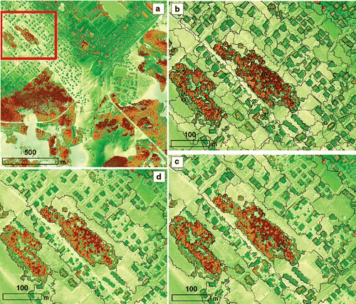
Figure 4. Mixed residential/forested test area: segmentation results at the lowest scale parameter (14) indicated by the ESP tool (middle). For comparison, see segmentation results at scale parameters 13 (left) and 15 (right). The following number of segments was generated of the respective scale parameters: 6896 (13), 6117 (14), and 5536 (15).

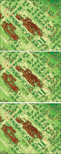
Figure 5. Natural savanna: segmentation results with scale parameters of 88 (a), 36 (b), and 16 (c). Patches of bare soil/grass are clearly delineated from individual trees and shrubs.

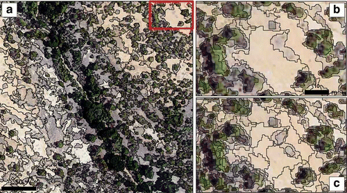
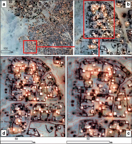
Figure 6. Temporary settlement area: The entire image as segmented (a) and the subset used for visualization (b). Traditional huts appear as dark gray/black whereas tents show up as bright white. Exemplary segmentation results were achieved with scale parameters of 18 (c) and 35 (d).

For the mixed residential/forested test area, we selected scale parameters of 14, 45, and 82 as indicated by the ESP tool (Figure 2a). These scale parameters correctly delineated three levels of image-objects representative of this subset (Figure 3): individual buildings (scale parameter 14), blocks of buildings (scale parameter 45), and broadest land cover classes as depicted by their heights (scale parameter 82). Scale parameters of 20 and 72 were less evident on this subset, but they mark levels in the vertical structure of forests, which are well represented in the bottom half of the scene (Figure 3).

For the same test area, we compared the segmentation results at the finest scale parameter indicated by the ESP tool with the subsequent lower and higher levels, respectively (Figure 4). Figure 4 confirms our assumption in Section 2: once segments match representative objects in real world (here individual houses), their boundaries are preserved along a number of scale levels, which slows down the general increase in LV. Indeed, it is visible in Figure 4 that boundaries of houses are not modified, although segmentation has been performed with nonhierarchical option. Objects in the background, however, became oversegmented at finer scale parameters (Figure 4b), and began to exceed the boundaries of the objects in the scene at coarser scale parameters (Figure 4a and b), causing some loss of details (Figure 4c).

Segmentations performed on the savanna riparian zone (Figure 5) and the temporary human settlement imagery (Figure 6) were equally good when the scale parameter settings suggested by ESP were used.

In Figure 5, a scale parameter of 16 produced segmentation at the level of individual trees and shrubs. A higher level of forest stands was produced with a scale parameter of 36, while an obvious separation between bare soils, grass, forests, and shrubs was achieved with a scale parameter of 88.

For the temporary settlement area, the focus was to find the suitable scale parameters for feature extraction, that is, extraction of two different dwelling types: (1) traditional (dark) huts and (2) bright tents. Therefore, only scales from 1 to 50 (Figure 2c) were tested. ESP outputs revealed that dark huts are best segmented with a scale parameter of approximately 18. Bright tents are oversegmented at this scale (Figure 6c), whereas at a scale parameter of 35 the tents are satisfactorily delineated (Figure 6d).

5. Discussion and conclusions

Although the production of multiscale representations of spatial entities has been technically enhanced in OBIA through image segmentation, choosing the suitable levels of representation has remained a challenge. What ‘suitable’ means depends primarily on how scale is conceptualized: as an inherent property of phenomena and their associated physical entities (and implicitly of their digital representations), or as a ‘window of perception’ (Marceau 1999). Building on the results of Kim et al. (2008), we used the concept of LV (Woodcock and Strahler 1987) to create a tool that informs suitable scale parameter selection for segmentation in Definiens Developer®.

The ESP tool has been tested at three sites on images of different data type (LiDAR, color photography, and QuickBird) and scene complexity (mixed residential/forest, savanna riparian zone, and desert settlement). The results in the three test areas confirm the findings of Kim et al. (2008) that the inherent data properties can be effectively used in detecting levels where segmentation results match structures in the real world. Kim et al. (2008) proved that LV graphs indicate the optimal scale parameter for delineating forest stands, when compared against manual delineation. The cited work focused on a single scale. In contrast to pixel-based approaches (Woodcock and Strahler 1987), where LV graphs peaked or declined, the LV graphs we obtained followed a relatively smooth variogram shape as in Kim et al. (2008). While appropriate for detecting a single scale, the LV graph is not suitable for a multiscale approach. That is why we introduced ROC-LV as a measure of LV dynamics across scales. The graph of ROC-LV enabled the detection of multiple scale parameters.

Segmentation results have been evaluated visually, based on expert knowledge. We decided upon using visual assessment only, as the human eye is acknowledged as ‘a strong and experienced source for evaluation of segmentation techniques’ (Baatz and Schäpe 2000, p. 15). Quantitative accuracy assessment would actually refer to classification, which falls beyond the scope of this paper. Quantitative assessment is particularly challenging in a multiscale approach, since it would rely on thematic resolution, which is still a subject of research (Castilla et al. 2009).

To date, the selection of appropriate scale parameter settings has been heavily dependent upon trial-and-error exploration. We aimed to speed up this process, all the while complying with current standards in evaluating segmentation outputs, that is, visual approximation in trial-and-error exploration. In this light, the ESP tool proved successful in determining the most suitable scale parameters for image segmentation. The object levels delineated with these scale parameters matched the structures in real world for all the test areas. The results shown here revealed that even minor changes in scale parameter (using a setting of 13 or 15 instead of 14) markedly alter the segmentation results, which exceeded our expectations. These results highlight the value of employing the ESP tool.

The hierarchy versus nonhierarchy option in the ESP tool helps targeting the application to the aim of the research. One example in this context is the difference between feature extraction and wall-to-wall classification. Thus, when focusing on feature extraction using OBIA, the ‘perfect’ scale is not as important as in wall-to-wall classifications. For feature extraction, as presented in the temporary settlement area, it is often sufficient to get a preliminary approximation of scale parameter. In the process of rule set development using CNL, the single features are reshaped and delineated starting from some initial scales in a cyclic process (‘class modeling’; cf. Tiede and Lang 2008). However, speed often being the most important factor in the extraction of these features (Tiede and Lang 2008), the ESP tool saves critical time by identifying initial scales for evaluation. Because the constraints from lower or upper levels impact on the shapes of features, the user might consider using the nonhierarchical option to avoid such issues.

The number of possible tessellations has increased infinitely in OBIA (Addink et al. 2007), requiring solutions to cope with finding appropriate parameters for image segmentation. The technique that we have developed will aid image analysts and researchers in selecting the most suitable range of scales for segmentation, thus enabling cost- and time-effective image analysis. This is particularly important for multiscale analysis as developed in some recent applications in various domains (Drăguţ and Blaschke 2006, 2008, Lamonaca et al. 2008, Levick and Rogers 2008, Lhermitte et al. 2008, Möller et al. 2008).

Besides the scale parameter, shape and compactness weighting might heavily impact on the segmentation results, particularly in classifications facing the challenge of spectrally similar objects (Luscier et al. 2006, Van der Werff and van der Meer 2008). The ESP tool offers the option of looking for the desired combination by iteratively running it with various combinations of shape and its attribute parameters.

So far, we have developed the ESP tool for application on a single layer, to make it independent of specific sensors or parametrization issues (Drăguţ et al. 2009). However, it can be adapted for multiple layers. Here we tested ROC-LV for scale ranges up to 100, with an increment of 1. Further research is needed to evaluate the sensitivity of this indicator to changes in scale ranges and increments. Since both scale range and increment are user defined in the ESP tool, we can expect more insights into this matter coming from specific applications.

Acknowledgements

The work of Lucian Dragut is supported by the Austrian Science Fund through a Stand-alone project (“SCALA”, FWF-P20777-N15) and by a Marie Curie European Reintegration Grant within the 7th EC Framework Programme (Grant agreement No. 239312). The work of Shaun R. Levick is funded by the Andrew W. Mellon foundation. Clemens Eisank has contributed to test the temporary settlement area. Data for the mixed residential/forest test area has been provided by the regional government of Salzburg (SAGIS, Land Salzburg). Data for the temporary settlement area has been exchanged within the frame of the EU-funded project LIMES (Land and Sea Integrated Monitoring for European Security, EC Sixth Framework Programme, Contract No. SIP-CT-2006-031046).

References

- Addink , E. , de Jong , S. and Pebesma , E. 2007 . The importance of scale in object-based mapping of vegetation parameters with hyperspectral imagery . Photogrammetric Engineering and Remote Sensing , 73 : 905 – 912 .
- Aplin , P. 2006 . On scales and dynamics in observing the environment . International Journal of Remote Sensing , 27 : 2123 – 2140 .
- Baatz , M. and Schäpe , A. 2000 . “ Multiresolution segmentation–an optimization approach for high quality multi-scale image segmentation ” . In Angewandte geographische informationsverarbeitung , Edited by: Strobl , J. , Blaschke , T. and Griesebner , G. 12 – 23 . Heidelberg : Wichmann-Verlag .
- Bauer , R. and Dahlquist , J. 1998 . Technical market indicators: analysis and performance , New York : Wiley .
- Benz , U.C. 2004 . Multi-resolution, object-oriented fuzzy analysis of remote sensing data for GIS-ready information . ISPRS Journal of Photogrammetry and Remote Sensing , 58 : 239 – 258 .
- Blaschke , T. 2003 . Object-based contextual image classification built on image segmentation . Advances in Techniques for Analysis of Remotely Sensed Data, 2003 IEEE Workshop , : 113 – 119 .
- Blaschke , T. and Strobl , J. 2001 . What's wrong with pixels? Some recent developments interfacing remote sensing and GIS . Zeitschrift für Geoinformationssysteme , 6 : 12 – 17 .
- Blaschke , T. , Lang , S. and Hay , G. 2008 . Object-based image analysis: spatial concepts for knowledge-driven remote sensing applications , Berlin : Springer-Verlag .
- Burnett , C. and Blaschke , T. 2003 . A multi-scale segmentation/object relationship modelling methodology for landscape analysis . Ecological Modelling , 168 : 233 – 249 .
- Castilla , G. 2009 . The impact of thematic resolution on the patch-mosaic model of natural landscapes . Landscape Ecology , 24 : 15 – 23 .
- Drăguţ , L. and Blaschke , T. 2006 . Automated classification of landform elements using object-based image analysis . Geomorphology , 81 : 330 – 344 .
- Drăguţ , L. and Blaschke , T. 2008 . “ Terrain segmentation and classification using SRTM data ” . In Advances in digital terrain analysis , Edited by: Zhou , Q. , Lees , B. and Tang , G.-A. 141 – 158 . Berlin : Springer .
- Drăguţ , L. 2009 . Optimization of scale and parametrization for terrain segmentation: an application to soil-landscape modeling . Computers and Geosciences , 35 : 1875 – 1883 .
- Fisher , P. 1997 . The pixel: a snare and a delusion . International Journal of Remote Sensing , 18 : 679 – 685 .
- Goodchild , M.F. , Yuan , M. and Cova , T.J. 2007 . Towards a general theory of geographic representation in GIS . International Journal of Geographical Information Science , 21 : 239 – 260 .
- Hall , O. 2004 . Detecting dominant landscape objects through multiple scales: an integration of object-specific methods and watershed segmentation . Landscape Ecology , 19 : 59 – 76 .
- Hay , G. , Niemann , K. and Goodenough , D. 1997 . Spatial thresholds, image-objects, and upscaling: a multiscale evaluation . Remote Sensing of Environment , 62 : 1 – 19 .
- Hay , G. 2005 . An automated object-based approach for the multiscale image segmentation of forest scenes . International Journal of Applied Earth Observations and Geoinformation , 7 : 339 – 359 .
- Kim , M. , Madden , M. and Warner , T. 2008 . “ Estimation of optimal image object size for the segmentation of forest stands with multispectral IKONOS imagery ” . In Object-based image analysis–spatial concepts for knowledge driven remote sensing applications , Edited by: Blaschke , T. , Lang , S. and Hay , G.J. 291 – 307 . Berlin : Springer .
- Lamonaca , A. , Corona , P. and Barbati , A. 2008 . Exploring forest structural complexity by multi-scale segmentation of VHR imagery . Remote Sensing of Environment , 112 : 2839 – 2849 .
- Lang , S. and Langanke , T. 2006 . Object-based mapping and object-relationship modeling for land use classes and habitats . Photogrammetrie, Fernerkundung, Geoinformation , 1 : 5 – 18 .
- Lees , B. 2006 . The spatial analysis of spectral data. Extracting the neglected data . Applied GIS , 2 : 14.1 – 14.13 .
- Levick , S.R. and Rogers , K.H. 2008 . “ Structural biodiversity monitoring in savanna ecosystems: integrating LiDAR and high resolution imagery through object-based image analysis ” . In Object-based image analysis–spatial concepts for knowledge driven remote sensing applications , Edited by: Blaschke , T. , Lang , S. and Hay , G.J. 477 – 491 . Berlin : Springer .
- Lhermitte , S. 2008 . Hierarchical image segmentation based on similarity of NDVI time series . Remote Sensing of Environment , 112 : 506 – 521 .
- Luscier , J.D. 2006 . Using digital photographs and object-based image analysis to estimate percent ground cover in vegetation plots . Frontiers in Ecology and the Environment , 4 : 408 – 413 .
- Marceau , D. 1999 . The scale issue in social and natural sciences . Canadian Journal of Remote Sensing , 25 : 347 – 356 .
- Marceau , D. and Hay , G. 1999 . Remote sensing contributions to the scale issue . Canadian Journal of Remote Sensing , 25 : 357 – 366 .
- Meinel , G. and Neubert , M. 2004 . “ A comparison of segmentation programs for high resolution remote sensing data ” . In Proceedings of 20th ISPRS Congress , Istanbul .
- Möller , M. 2008 . Placing soil-genesis and transport processes into a landscape context: a multiscale terrain-analysis approach . Journal of Plant Nutrition and Soil Science , 171 : 419 – 430 .
- Ryherd , S. and Woodcock , C. 1996 . Combining spectral and texture data in the segmentation of remotely sensed images . Photogrammetric Engineering and Remote Sensing , 62 : 181 – 194 .
- Schiewe , J. , Tufte , L. and Ehlers , M. 2001 . Potential and problems of multi-scale segmentation methods in remote sensing . GIS – Zeitschrift fur Geoinformationssysteme , 6 : 34 – 39 .
- Silván-Cárdenas , J.L. , Wang , L. and Zhan , F.B. 2009 . Representing geographical objects with scale-induced indeterminate boundaries: a neural network-based data model . International Journal of Geographical Information Science , 23 : 295 – 318 .
- Smith , G. 2007 . UK land cover map production through the generalisation of OS MasterMap (R) . Cartographic Journal , 44 : 276 – 283 .
- Strahler , A.H. , Woodcock , C.E. and Smith , J.A. 1986 . On the nature of models in remote sensing . Remote Sensing of Environment , 20 : 121 – 139 .
- Tiede , D. and Hoffmann , C. 2006 . “ Process oriented object-based algorithms for single tree detection using laser scanning ” . In International workshop ‘3D Remote Sensing in Forestry’ , Edited by: Koukal , T. and Schneider , W. 162 – 167 . Vienna .
- Tiede , D. Lang , S. 2008 . “ Rapid dwelling extraction from VHSR satellite imagery in refugee camps and dissemination of conditioned information via virtual globes ” . In Digital Earth Summit on Geoinformatics 2008: tools for global change research , Edited by: Ehlers , M. 100 – 105 . Heidelberg : Wichmann .
- Van Der Werff , H.M.A. and Van Der Meer , F.D. 2008 . Shape-based classification of spectrally identical objects . ISPRS Journal of Photogrammetry and Remote Sensing , 63 : 251 – 258 .
- Woodcock , C. and Strahler , A. 1987 . The factor of scale in remote sensing . Remote Sensing of Environment , 21 : 311 – 332 .