Spatiotemporal data model for network time geographic analysis in the era of big data

ABSTRACT

There has been a resurgence of interest in time geography studies due to emerging spatiotemporal big data in urban environments. However, the rapid increase in the volume, diversity, and intensity of spatiotemporal data poses a significant challenge with respect to the representation and computation of time geographic entities and relations in road networks. To address this challenge, a spatiotemporal data model is proposed in this article. The proposed spatiotemporal data model is based on a compressed linear reference (CLR) technique to transform network time geographic entities in three-dimensional (3D) (x, y, t) space to two-dimensional (2D) CLR space. Using the proposed spatiotemporal data model, network time geographic entities can be stored and managed in classical spatial databases. Efficient spatial operations and index structures can be directly utilized to implement spatiotemporal operations and queries for network time geographic entities in CLR space. To validate the proposed spatiotemporal data model, a prototype system is developed using existing 2D GIS techniques. A case study is performed using large-scale datasets of space-time paths and prisms. The case study indicates that the proposed spatiotemporal data model is effective and efficient for storing, managing, and querying large-scale datasets of network time geographic entities.

KEYWORDS:

• Time geography
• spatiotemporal data model
• spatiotemporal query
• spatiotemporal big data
• compressed linear reference

1. Introduction

Time geography is a powerful framework for studying human activities under various space-time constraints. The framework provides a set of well-defined space-time entities (e.g., space-time path and prism) and relations (e.g., bundling and intersections) to analyze human activities in space and time. It has served as a fundamental analytical framework for many scientific fields, such as transport geography and urban planning (Huang and Wu 2008, Fang et al. 2011, 2012, Kwan 2013, Versichele et al. 2014, Charleux, 2015).

The concept of time geography was first introduced by Torsten Hägerstrand in the 1960s (Hägerstrand 1970). In early studies, time geography was qualitative and lacked formal and analytical statements of basic entities and relations (Long and Nelson 2013). With the availability of geographical information science (GIS) tools, the last two decades have witnessed a resurgence of time geography. Research efforts have focused on establishing measurement theory and developing computational tools for quantitative time geographic analysis (Kwan and Weber 2003, Miller 2005). Recognizing that people in urban area are generally traveling within networks, researchers have extended the time geographic framework from planar space to constrained network space and considered the complexities of traffic conditions in networks (Miller 1991, Neutens et al. 2008, Miller and Bridwell 2009, Chen et al. 2013). Geo-visualization tools integrated with GIS platforms also have been developed to explore human activity and travel patterns (Kwan 2000, Yu and Shaw 2008, Shaw and Yu 2009, Chen et al. 2011).

In recent years, there has been a wider resurgence of interest in time geography due to the increasing availability of spatiotemporal Big Data in urban environments. The recent development of information and communication technologies (ICTs) has made it technically and economically feasible to collect large-scale individual movement data. Fine gained movement data include taxi trajectories, mobile phone records, smart card data, social media check-ins, and various user-generated geographical information (Li et al. 2013, Yue et al. 2014). Spatiotemporal Big Data offers an unprecedented opportunity for time geographic studies to uncover people’s mobility patterns and their interactions with the urban environment (Song et al. 2010, Goodchild 2013, Richardson et al. 2013, Kwan and Neutens 2014, Pei et al. 2014). However, the rapid increase in the volume, diversity, and intensity of movement data poses a significant challenge to contemporary GIS platforms with respect to the representation and computation of time geographic entities and relations. To address this challenge, the present study proposes an effective spatiotemporal data model with capability to store, manage, and analyze large movement datasets and thereby support large-scale time geographic analysis.

The integrated representation of spatial and time is an active frontier in GIS research. Many spatiotemporal data models have been proposed to represent discrete changes of geographical phenomena (e.g., landuse changes), including snapshot model (Armstrong 1988), spatiotemporal composite model (Langran and Chrisman 1988), event-based spatiotemporal data model (Peuquet and Duan 1995), three-domain data model (Yuan 1999), geo-atom model (Goodchild et al. 2007, Chen et al. 2012), object-oriental models (Wang and Cheng 2001), among others. However, these spatiotemporal data models are not tailored to the representation of time geographic entities and relations.

Effective storage and management of movement data have also inspired a large amount of literature on moving objects databases. Research regarding moving objects databases started from the work of Güting (Erwig et al. 1999) and Wolfson (Wolfson et al. 1998). Effective designs of moving objects databases have been proposed for storing, indexing, and querying movement data in unconstrained planar space (Güting and Schneider 2005). Research efforts have recently focused on extending moving objects databases to constrained network space (De Almeida and Güting 2005, Güting et al. 2006, Li and Lin 2006, Xu and Güting 2013; Popa et al. 2015). While current moving objects databases can offer efficient methods for storing and retrieving movement data, they seldom integrate with the GIS platforms. Moreover, current moving objects databases only model the space-time path entity, ignoring other time geographic entities (e.g., space-time prism) and relations (e.g., path-prism and prism-prism intersections). Therefore, current moving objects databases are not suitable for large-scale time geographic analysis.

To fill the gap, the present study proposes a spatiotemporal data model for large-scale time geographic analysis. The proposed spatiotemporal data model is based on a compressed linear reference (CLR) technique to transform network time geographic entities in three-dimensional (3D) (x, y, t) space to two-dimensional (2D) CLR space. Using the proposed model, network time geographic entities (i.e., space-time paths, stations, prisms, and lifelines) can be stored and managed in classical spatial databases. Efficient spatial operations and index structures can be directly utilized to implement spatiotemporal operations and queries for network time geographic entities in CLR space. To validate the proposed model, a prototype system is developed using existing 2D GIS techniques. A real-world case study is also performed using large-scale datasets of space-time paths and prisms. The case study indicates that the proposed spatiotemporal data model is effective and efficient for storing, managing, and querying large-scale datasets of network time geographic entities.

Section 2 briefly introduces time geographic entities and relations in the planar space (Miller 2005) to provide the necessary background. Section 3 introduces the representation of network time geographic entities and relations in CLR space. Section 4 presents the proposed spatiotemporal data model, associated spatiotemporal database design, and spatiotemporal queries. Section 5 details a case study to illustrate the applicability of the proposed model. Section 6 concludes the article with possible directions for future research.

2. Time geographic entities in planar space

The space-time path and prism are two entities central to time geography. The space-time path (also called trajectory in the literature) traces the movement of an individual in space and time. As illustrated in Figure 1, it is represented by a space-time polyline in (x, y, t) space with two spatial axes for geographic space and a third orthogonal axis for time. The (x, y, t) space is also known as the space-time cube (Kwan 2000, Nakaya 2013). The space-time path of the individual comprises a set of control points and a corresponding sequence of path segments connecting these points (Miller 2005). Typically, the control points are observation records collected by location-aware technologies (LAT) such as GPS devices. Each control point, , consists of the triple

(1)

Figure 1. Space-time paths in planar space.

where and are spatial coordinates, and is a time stamp. It is commonly assumed in the literature that the individual is moving at a constant speed between each of the two adjacent control points, and (Wolfson et al. 1998, Miller 2005). Using this assumption, the path segment between and is a straight line

(2)

The speed of path segment is

(3)

where is the Euclidian distance between two locations. A vertical path segment indicates that the individual is stationary in space, perhaps participating in activities. The space-time path therefore can be expressed as a 3D LineString comprising a set of straight line segments

(4)

The individual’s location on the space-time path at any time stamp can be determined from

(5)

In principle, representing the space-time path as straight line segments (i.e., the assumption of constant speed between two adjacent control points) can capture complete information of a trajectory by collecting every location with direction and speed changes. However, in practice, movement data are usually collected at regular or irregular time intervals, and the resolution of a space-time path depends on its sampling frequency.

The space-time station, , also illustrated in Figure 1, is a vertical space-time path

(6)

It generally refers to an activity location, (e.g., store, cinema, restaurant, etc.) where space-time paths can bundle or cluster in space and time. The finite durations of the station refer to time periods when the activity location is available (e.g., store operating hours).

Given an origin and a destination , the space-time prism () delimits the space-time extent for an individual to conduct discretionary travel from and reach . Figure 2 illustrates this space-time prism in planar space. The space-time prism is commonly used for activity scheduling and accessibility analysis. The two control points (also called anchor points), generally obtained from activity diary data, represent an individual’s fixed activities, such as home, work, or meetings. Between two fixed activities, a flexible activity may be scheduled by the individual at location and time with minimum duration . Let be the minimum travel time from the origin to location . The earliest arrival time at the flexible activity location can be simply calculated by

(7)

Figure 2. A space-time prism in planar space.

where is the maximum travel speed. To arrive at destination on time, the latest departure time from location can be calculated by

(8)

where is the minimum travel time from to the destination. This location is feasible for activity participation if the following constraint is satisfied:

(9)

Therefore, the potential path area (PPA) delimiting all potential locations for activity participations is defined as

(10)

The space-time prism is a 3D prism-shaped structure capturing all potential space-time locations for an individual to conduct the flexible activity, and can be expressed as the intersection of a forward cone, a backward cone, and a cylinder:

(11)

(12)

(13)

(14)

where is the forward cone comprising all space-time locations that can be reached from origin by elapsed time ; is the backward cone encompassing all space-time points where an individual can return to destination in the remaining time budget ; and is the cylinder delimiting all reachable geographic locations. The footprint of the 3D prism in geographical space is the PPA. The potential locations of the individual at a given time instance are a subset of PPA,

(15)

where indicates the logical predicate AND. The height of the space-time prism at any location is the time resource available for activity participations determined by the earliest arrival and latest departure times,

(16)

Figure 2 also shows the connection between the space-time path and prism. The space-time path represents a revealed movement of activity participation, while the space-time prism delimits all possible movements between two control points. Analyzing an individual’s activities may require a combination of several space–time paths and prisms into a composite object, the space-time lifeline (Miller 2005). Figure 3 illustrates a simple space-time lifeline with one space-time path and two space-time prisms. The space-time lifeline is represented by the combination of space–time paths and prisms,

(17)

Figure 3. A space-time lifeline in planar space.

In addition to space-time entities, time geography defines two basic space-time relations, namely intersections and bundles. Intersections are where two or more time geographic entities co-exist in space and time. As shown in Figure 4, they can be classified into path-path, path-prism, and prism-prism intersection cases. Space-time intersections are important to time geographic analysis. For example, a joint activity cannot be scheduled for two entities unless their space-time prisms intersect.

Figure 4. Space-time intersections.

Bundles are path-path relations, with respect to the convergence of space-time paths for some shared activities. As illustrated in Figure 5, bundling of space-time paths does not require co-existence of paths in space and time but allows a spatial tolerance at any time instance. Path bundling is useful for monitoring crowd dynamics at large events or identifying an individual’s activities from his multi-day paths.

Figure 5. Space-time path bundling.

The representation of time geographic entities by 3D lines and/or volumes in (x, y, t) space is rigorous and analytical (Miller 2005). However, this representation technique poses significant challenges to contemporary 2D GIS and database platforms for efficiently storing, querying, and analyzing large-scale time geographic entities (Nakaya 2013, Kwan and Neutens 2014).

3. Representation of network time geographic entities and relations

People in urban areas do not move freely in (x, y, t) space, but rather within spatially embedded road networks. In this section, we present a spatiotemporal data model for network time geographic entities and relations, which enables more efficient time geographic analysis.

A road network can be represented as a directed graph, , comprising a set of nodes , and a set of links . Each link, , has a set of attributes including identity, ; length, ; and travel time, . To guarantee link uniqueness, link ID is set as a unique positive integer number. A link, , has a starting node, ; an ending node, ; and a set of intermediate vertices, . The link geometry is represented by a set of link segments connecting each two adjacent vertices in the link.

In addition to geographical coordinates, a location in the road network can be referenced in a natural and convenient way using a linear reference system (LRS) (Miller and Shaw 2001). The LRS has been widely used in transportation applications, such as recording traffic incidents and transportation infrastructures. A location, , on link can be represented as , where is the relative position on the link, and indicates the middle of the link. The values and, respectively, refer to the starting and ending nodes of the link, where is a very small tolerance (say ). The linear reference is an equivalent representation of the geographical location in the road network (with the one-to-one relationship). The geographical location can also be determined from using the dynamic segmentation technique (Miller and Shaw 2001).

Since linear measurement, , is a real number between 0 and 1, and link ID, , is a unique positive integer number, a CLR technique is proposed by integrating and into a single value:

(18)

For example, control point shown in Figure 6 locates on link 5 with , and this network location is referenced as using the CLR technique. It is apparent that the value is also an equivalent representation of the geographical location in the road network and can be easily transformed to the geographical location using the dynamic segmentation technique.

Figure 6. A network space-time path in (x, y, t) space.

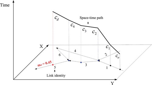
Using the CLR technique, any space-time location, , on link can be referenced in (z, t) space by

(19)

For example, the control point shown in Figure 6 can be represented as in (z, t) space. In this way, the proposed CLR approach represents network time geographic entities as 2D elements in (z, t) space, which makes it possible to utilize existing 2D GIS platforms for storing and managing network time geographic entities. For convenience, (z, t) space is referred as CLR space hereafter.

3.1. Network space-time path and station in CLR space

Figure 6 illustrates a network space-time path in the (x, y, z) space. Unlike planar space, movements in the road network are restricted by road geometry and traffic regulations (e.g., turn restrictions). To reflect road geometry in the space-time path, network nodes and intermediate vertices are required as control points. As shown in Figure 6, the network space-time paths should include not only observation locations (, and ) but also network nodes ( and ) and an intermediate vertex () as control points. In practice, observations are seldom collected at network nodes and intermediate vertices, and control points at these locations are generally estimated by linear interpolation (Equation (5)), assuming that the individual is moving at a constant speed between two adjacent observations.

Figure 7 illustrates the space-time path in CLR space using the same movement data shown in Figure 6. The space-time path is represented in CLR space by a set of disjoint LineString (i.e., polyline) elements

(20)

Figure 7. A network space-time path in CLR space.

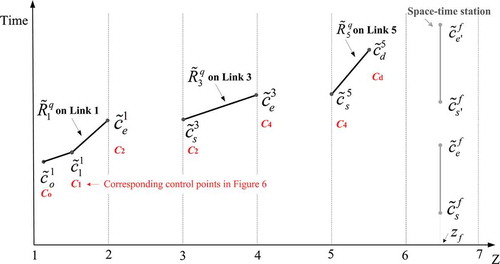
where the LineString element corresponds to a continuous movement on link . For example, the space-time path shown in Figure 7 consists of three LineString elements (, , and ) representing movements on Links 1, 3, and 5, respectively. Although the space-time path is continuous in (x, y, t) space, the LineString elements are disjoint in CLR space.

Each LineString element, , comprises a set of control points, , in CLR space, including at starting node , at ending node , and an arbitrary number of control points for LAT observations. All control points in are converted from corresponding control points in (x, y, t) space using the CLR technique. For example, , , and in Figure 7 are converted from , , and, respectively, in Figure 6. Note that control points at intermediate vertices (e.g., in Figure 6) are no longer needed in to maintain road geometry. This can be important to reduce data volume for large-scale movement data.

In LineString element , a straight line segment is connected between each of two subsequent control points and . The speed of the line segment is

(21)

where and are decimal parts of and , respectively; and is the link length. Thus, LineString element can be expressed as one or more straight line segments,

(22)

The LineString element has at least one straight line segment between the starting node, , and the ending node, . For each line segment, , the z value at any time stamp is determined by

(23)

Then, the location at any time stamp in the space-time path can be determined from piecewise linear interpolation

(24)

We can prove that at any time stamp the location is equivalent to the corresponding location in (x, y, t) space as follows.

Proposition 1.

The space-time path in CLR space is an equivalent representation of space-time path in (x, y, t) space.

Proof.

From the definition of , all control points, , at network nodes and observations in CLR space are converted from the corresponding control points in . Thus, at these control points, is equivalent to . For any time stamp between two control points, and , is determined by linear interpolation (Equation (24)). Since any space-time location between two observations is also estimated by linear interpolation in , is also equivalent to . □

Figure 7 also illustrates the space-time station in CLR space (denoted by ). The space-time station is represented in CLR space by a set of disjoint vertical LineString elements

(25)

Each LineString element, , refers to an available time duration, , at activity location, . It can be expressed as a vertical line segment, , between two control points, and . The space-time station is stationary for the available time durations as

(26)

Lemma 1.

The space-time station in CLR space is an equivalent representation of space-time station in (x, y, t) space.

Proof.

It is apparent that is equivalent to , since it is stationary during all available time periods. □

3.2. Network space-time prism and lifeline in CLR space

Space-time prisms in the road network are restricted by the road geometry. In the road network, the shortest distance between any two locations and is not Euclidean distance but the network distance, denoted by , which can be calculated by the shortest path algorithms (Li et al. 2015). To represent the essential ideas of network space-time prisms, it is assumed that U-turn is not allowed along any network link. This assumption is reasonable for major divided roads. For minor undivided roads, such assumption can be relaxed according to Kuijpers and Othman (2009).

Figure 8 illustrates the network space-time prism in (x, y, t) space using and as anchor points. The network space-time prism is a 3D element in (x, y, t) space delimiting all accessible space-time locations in the road network. Since network links are 1D linear features, the network space-time prism comprises a set of 2D polygons; each of which represents the potential space-time locations on a corresponding network link. Let denote the 2D space-time polygon in (x, y, t) space on link . The network space-time prism can be represented as a set of space-time polygons in (x, y, t) space

(27)

Figure 8. A network space-time prism in (x, y, t) space.

For example, the network space-time prism shown in Figure 8 consists of five polygons in space and time (, , , , and ).

Each space-time polygon, , comprises a set of control points at starting node , ending node , and all intermediate vertices, . For each node (or vertex), two controls, and , are constructed at its earliest arrival time, , and latest departure time, , respectively. The space-time polygon, , is represented by a ring connecting all control points in clockwise order:

(28)

where is the line segment connecting two control points and .

Solution algorithms have been proposed in the literature to generate the network space-time prism by explicitly constructing space-time polygons based on forward and backward path searches from and , respectively (Miller 1991, Chen et al. 2013). If two anchor points, and , are not at network nodes, two dummy nodes, and , would be added to the road network. The forward shortest path search determines the least travel time from the starting anchor point, , to each network node, , while the backward search determines the least travel time from each network node, , to the ending anchor point, . The accessible link can be determined from constraints and . For starting node on each link , the earliest arrival time, , and the latest departure time, , are calculated to construct control points and . The earliest arrival time, , and latest departure time, , at the ending node, , are then obtained to construct control points and . The earliest arrival time, , and latest departure time, , at every intermediate vertex, , are obtained to determine and , where is the relative position of the vertex along link . After all control points are constructed, the space-time polygon, , is generated for each accessible link .

As shown in Figure 8, the projection of the network space-time prism onto geographical space is the potential network area (PNA) in terms of accessible links. It can be defined as those links with starting and ending nodes satisfying time constraints:

(29)

Given any location on link , its earliest arrival time and latest departure time can be determined by

(30)

where is the relative position of location along link . The potential locations of the individual at a given time instance are a subset of PNA,

(31)

The height of the space-time prism at any location on link is determined by its earliest arrival time and latest departure time

(32)

Figure 9 illustrates the network space-time prism in CLR space using the same settings as Figure 8. The two anchor points are and in CLR space. As shown in the figure, the network space-time prism in CLR space () comprises a set of 2D polygons:

(33)

Figure 9. A network space-time prism in CLR space.

where each polygon, , corresponding to a space-time polygon, , in (x, y, t) space, delimits all potential space-time locations on the link . For example, the network space-time prism shown in Figure 9 consists of five polygons in CLR space (, , , , and ) corresponding to the five space-time polygons in Figure 8.

Each polygon consists of only four control points in CLR space. Two control points and refer to the earliest arrival time, , and the latest departure time, , at the starting node, , respectively. The other two control points, and , correspond to the earliest arrival time, , and the latest departure time, , at the ending node, , respectively. All four control points can be transformed from the corresponding control points in in (x, y, t) space using the CLR technique. Control points at intermediate vertices are no longer needed in to represent road geometry. Thus, the space-time polygon, , can be represented by a ring connecting four control points in clockwise order:

(34)

where is the line segment connecting two control points, and .

The network space-time prism in CLR space, , can be constructed by existing solution algorithms based on forward and backward shortest path searches. Using the results of shortest path searches, the earliest arrival time, , and the latest departure time, , can be calculated, to construct and at starting node on each accessible link . The earliest arrival time, , and latest departure time, , at ending node can then be calculated, to construct control points and . After constructing these four control points , the space-time polygon, , on accessible link is generated. Consequently, the space-time prism, , is constructed by generating space-time polygons for all accessible links.

The projection of the space-time prism onto the z-axis is the PNA in terms of linear events . Each linear event, , represents an accessible link, , in CLR space. Thus, the PNA in CLR space () can be expressed as

(35)

Given at any location, , on link , its earliest arrival time, , and latest departure time, , can be determined by

(36)

where is the decimal part of . The potential locations of the individual at a given time stamp, , are a subset of PNA:

(37)

We can prove that the potential locations in at any time stamp are equivalent to corresponding locations in in (x, y, t) space as follows.

Proposition 2.

The network space-time prism in CLR space is an equivalent representation of the network space-time prism in (x, y, t) space.

Proof.

From the definition of , four control points, , at network nodes of each space-time polygon are converted from corresponding control points, , in using the CLR technique. Therefore, the earliest arrival time, , and the latest departure time, , at the starting node in are identical to that in . Comparing Equations (36) and (30), we have the earliest arrival time, , and the latest departure time, , at any location in CLR space identical to that at corresponding location in (x, y, t) space. Since and are identical at any location in the network, the potential locations in are therefore equivalent to from Equations (37) and (31). □

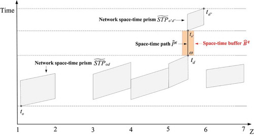
Figure 10 illustrates a simple network space-time lifeline in CLR space. The illustrated space-time lifeline is a combination of a space-time path and two network space-time prisms in CLR space. The network space-time prism is a 2D entity, while the space-time path is 1D (linear) entity. Since it is difficult to represent different dimensional entities in a feature, every space-time path in the lifeline is converted into 2D entity using spatiotemporal buffering. Given a space-time path and a spatial tolerance , this operation creates a spatial buffering on the individual’s location, , any time stamp, . An adoptive spatial tolerance can also be used for links with different lengths, where is the link length and is threshold value in percentage. The result of spatiotemporal buffering (space-time buffer, ) is the space-time regions within which the distance of any location to is less than tolerance as

(38)

Figure 10. A network space-time lifeline in CLR space.

where is the network distance from location to location . The space-time buffer consists of a set of space-time polygons, , and each represents the space-time regions on link . The detailed algorithm for spatiotemporal buffering operation in CLR space is described in Chen et al. (2015).

After all space-time paths are converted into space-time buffers using a very small spatial tolerance, , the space-time lifeline in CLR space, , can be represented by a set of 2D space-time polygons from both space-time buffers and prisms:

(39)

Lemma 2.

The space-time lifeline, , in CLR space is an equivalent representation of space-time lifeline, , in (x, y, t) space.

Proof.

The space-time lifeline, , in (x, y, t) space is a combination of space-time paths and prisms. From Proposition 2, all space-time prisms in in CLR space are equivalent representations of corresponding prisms in (x, y, t) space. From the definition of , all space-time paths are converted to space-time buffers by spatiotemporal buffering using a very small spatial tolerance. Thus, space-time buffers in can approximate the space-time paths in CLR space. From Proposition 1, these space-time buffers are equivalent representations of corresponding space-time paths in (x, y, t) space. Therefore, the space-time lifeline, , is an equivalent representation of in (x, y, t) space. □

3.3. Network time geographic relations in CLR space

As noted earlier, space-time intersection and path bundling are two key space-time relationships in time geography. Table 1 shows the space-time intersections for network time geographic entities in CLR space. Since the space-time paths (and stations) are 1D entities and the space-time prisms (and lifelines) are 2D entities in CLR space, thus space-time intersections can be classified into path-path, path-prism, and prism-prism cases. All these space-time intersection problems in CLR space can be equivalently solved by classical spatial intersection in 2D space (Egenhofer and Herring 1990).

Table 1. Space-time intersections of network time geographic entities in the CLR space.

Relations	Path-path	Path-prism	Prism-prism
A contains B
A within B
A touches B
A overlaps B		–
A crosses B

As shown in Table 1, the space-time intersections in this study are further refined into five space-time sub-relations: Contains, Within, Touches, Overlaps, and Crosses. Contains is the condition that Entity A wholly contains Entity B. For example, space-time Path B shown in the table is a feasible schedule for an individual, because the individual’s space-time Prism B contains the path. Within is the complementary condition that Entity A is wholly contained within Entity B. Touches refers to the condition of Entity A’s ending point meeting Entity B’s starting point. For example, an individual’s space-time Prism A in the table touches his space-time Path B indicating that a fixed activity (i.e., path) would be carried out after a flexible activity (i.e., prism). Overlaps is a space-time relation of same dimension entities (i.e., path-path and prism-prism), and refers to the coincidence of entities A and B for a time period. For example, a joint activity can be scheduled only at space-time locations where space-time Prism A overlaps Prism B, as shown in the table. Crosses is valid for all path-path, path-prism, and prism-prism cases. It refers to where the intersection of the two entities has a lower dimension than the maximum dimension of the entities. For the path-path case, Crosses refers to the coincidence of entities A and B at certain time instances except for the Touches conditions. For the path-prism case, Crosses is the condition of Entity A intersecting Entity B for certain time periods or time instances except for the Touches and Contains conditions. For the prism-prism case, the Crosses is the condition that the intersection of two prisms is one or more 1D space-time paths.

Path bundles correspond to the convergence of space-time paths in space and time. Bundling very often occurs at some stations, implying that the individuals are participating in shared activities at the stations. Paths can also bundle during the movements, such as taking the same bus. Unlike space-time intersections, bundling of two space-time paths and for a time period, , does not require exact co-existence of these two paths in space but allows a spatial tolerance, . Thus, these two paths should satisfy for any time instance , where is the network distance between two locations.

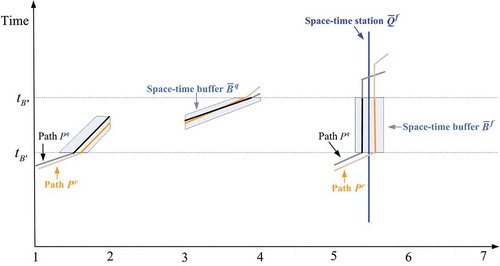
As shown in Figure 11, using spatiotemporal buffering, path bundling can be solved as a space-time intersection problem. Given a spatial tolerance, , a space-time buffer, , can be generated for a space-time station, , during the time period . The generated space-time buffer delimits all space-time locations whose network distance to station at any time instance, , is less than the spatial tolerance. Therefore, all space-time paths bundling at the station can be determined by the Contains relation as those paths contained by the space-time buffer during the time period . Similarly, paths bundling during the movements can also be determined by generating space-time buffer for the movement during the time period . The paths bundling with the target path are those paths contained by the space-time buffer, , during the time period (e.g., in Figure 11). The detailed algorithm for generating space-time buffers in CLR space is given in Chen et al. (2015).

Figure 11. Paths bundling in CLR space.

4. Spatiotemporal data model for network time geographic entities in CLR space

This section presents the spatiotemporal data model, associated spatiotemporal database design, and spatiotemporal queries based on the aforementioned representations of network time geographic entities and relations in CLR space.

4.1. Spatiotemporal data model

Figure 12 shows the class diagram of the spatiotemporal data model for network time geographic entities in CLR space. To integrate with existing GIS platforms, the OpenGIS simple features access standard (Herring 2011) is adopted to represent classical 2D spatial features (i.e., Geometry, Point, MultiPoint, LineString, MultiLineString, Polygon, and MultiPolygon). As shown in the figure, ClrSpaceTimePath, ClrSpaceTimeStation, ClrSpaceTimePrism, ClrSpaceTimeLifeLine, and ClrSpaceTimeBuffer represent the space-time path, station, prism, lifeline, and buffer entities, respectively, in CLR space. A ClrObservations object is also introduced to represent discrete LAT observations. These space-time entities are all derived from the Geometry object, implying that they are special types of 2D spatial objects in CLR space. The space-time path and station entities are represented by a MultiLineString object comprising a set of LineString objects. The space-time prism, lifeline, and buffer entities are formulated by a MultiPolygon object consisting of one or more Polygon objects.

Figure 12. Spatiotemporal data model for network time geographic entities in CLR space.

4.2. Spatiotemporal database design

Based on the aforementioned spatiotemporal data model, the network time geographic entities can be stored and managed in classical spatial databases, such as ESRI Geodatabase or Oracle Spatial. Thus, space-time entities with the same dimension can be organized and stored as a feature class (or a layer). For example, space-time prisms of a collection of individuals are organized as a polygon feature class and each record of the feature class is the space-time prism of an individual. In addition to the spatiotemporal shape, semantic information can be stored as attributes in the feature class, such as individuals’ age, sex, occupation, etc. Since spatial database techniques are adopted, traditional spatial datasets, including road networks, can be stored and managed in the same database. This makes it easy to integrate time geographic analysis with the powerful visualization and spatial analysis capabilities provided by contemporary GIS platforms (Kwan 2000).

Since the network time geographic entities are modelled as 2D features in CLR space, the numerous spatial operations developed for contemporary GIS platforms can be directly utilized to implement the spatiotemporal operations of network time geographic entities. For example, the spatial relational operators (i.e., IRelationalOperator) provided in ArcGIS can be directly employed to determine if a certain space-time intersection relationship defined in Table 1 exists between two time geographic entities. The Intersect function of ITopologicalOperator in ArcGIS can be utilized to obtain the intersection result of two time geographic entities. The use of well-developed spatial operations provides an effective approach for quickly developing time geographic analysis applications. Importantly, this approach can lead to more efficient time geographic analysis, because it is always computationally simpler to manipulate entities in 2D CLR space than the higher dimensional (x, y, t) space.

The well-developed spatial index technique can also be directly employed to construct the spatiotemporal index for quick retrieval of network time geographic entities in the database. Many existing spatial index structures from the literature can be used, including R-tree (Guttman 1984), Quad-tree (Finkel and Bentley 1974), and Grid-file (Nievergelt et al. 1984).

4.3. Spatiotemporal queries

Based on the spatial database and index techniques, spatiotemporal queries on time geographic entities can be easily implemented using the spatial query technique. Similar to traditional spatial queries, one requires an input space-time geometry and to choose a space-time relation defined in Table 1 (or roughly the intersection relation representing any space-time intersection relation). Using different values of these two parameters, various spatiotemporal queries can be performed to retrieve the time geographic entities stored in the database. Some typical spatiotemporal queries are as follows.

1. Path-path intersection query. Given a space-time path, , of an individual, find all space-time paths intersecting the path.

   This spatiotemporal query retrieves all individuals who physically meet the given individual. The query can be easily implemented in CLR space using a spatial intersect query on a space-time path layer with as the input geometry.

2. Window-path intersection query. Given a spatial window, W = (,,,), and a time period, [,], find all space-time paths intersecting the spatial region during the time period to .

   This spatiotemporal query finds all individuals who exist in the spatial region W during the time period from to . The query can be implemented in four steps: (1) a spatial query is performed on the road network to retrieve all network links intersecting the input spatial window W. (2) The set of linear events, , is determined within the spatial window for all retrieved networks. (3) A space-time region, , in CLR space is constructed by generating a set of space-time polygons, . Each space-time polygon is determined by four control points , , , and on a linear event, [,], during the time period [,]. (4) A spatial intersect query is performed on space-time paths layer using as the input geometry.

3. Station-prism within query. Given a location, , and a time period, [,], find all space-time prisms containing the location for the time period [,].

   This spatiotemporal query finds all individuals who could feasibly conduct an activity at given location, , during the time period from to . The query can be easily implemented in CLR space using a spatial Within query on a space-time prism layer. The input geometry is a space-time station at for the time period [,].

4. Prism-prism intersection query. Given a space-time prism, , of an individual, find all space-time prisms that intersect with the given prism .

   This spatiotemporal query finds all individuals who are feasible to conduct a joint activity with the given individual. The query can be easily implemented in CLR space using a spatial Intersect query on a space-time prism layer with as the input geometry.

5. Experimental evaluation

This section presents a case study using a real-world large-scale LAT observation data to demonstrate the applicability of the proposed spatiotemporal data model. In this study, the ArcGIS Geodatabase data model, which follows the OpenGIS simple features access standard, was used to implement the proposed spatiotemporal data model. ArcSDE 10.2 and Oracle 11g were adopted as the spatial database, which utilize the Grid-file index structure as the spatial index. In the database, Double data type was used for storing x, y, t, and z elements. Spatiotemporal queries were implemented in the ArcEngine 10.2 development kit using Microsoft Visual C#. All experiments were conducted on a desktop computer with an Intel dual core 3.1 GHz CPU, 8 GB RAM, running the Windows 7, 64-bit operating system.

5.1. Data description

Three real-world datasets in Shenzhen city, China, were collected for this case study. The first dataset was the Shenzhen road network, as shown in Figure 13, which consists of 69,198 nodes and 192,582 directed links. The identities of the network links are unique and range from 1 to 192,582. The road network was stored in the database as a road layer and an R-tree index was built for quickly retrieving the network links. The road network serves as a reference framework in CLR space for converting locations in (x, y, t) space to CLR space and vice versa. The distance (or travel time) between any two locations in CLR space can be calculated by the shortest path algorithm in the road network (Huang et al. 2007, Li et al. 2015). To facilitate these calculations, the road network was loaded into memory.

Figure 13. Shenzhen road network.

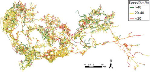
The second dataset was Shenzhen floating car data. The floating car system in Shenzhen consists of about 15,000 taxis equipped with GPS devices to record their locations approximately every 30 seconds. Due to GPS positioning errors and the abstract representation of the road network, GPS observations of a taxi may not be exactly on network links. To address this, a multi-criteria dynamic programming map matching (MDP-MM) algorithm (Chen et al. 2014) was employed to accurately match the observations onto the road network. Since a relatively low frequency was used in the collected dataset, a taxi may have passed through several network links between two adjacent observations. The missing network nodes in the taxi trajectories can be imputed by the MDP-MM algorithm. After the map-matching process, all taxi trajectories were converted into CLR space and stored as a space-time path layer. The conversion of space-time paths from (x, y, t) space to CLR space did not introduce additional computational effort, because the z value of each GPS observation was already determined in the map matching process. Consequently, the trajectories of 13,445 taxis collected on a typical weekday (11 May 2012, a Friday) during a 1-hour period (8–9 a.m.) were converted into space-time paths in CLR space and stored in the spatial database as a polyline layer.

The collected taxi space-time paths were also utilized to estimate the traffic conditions of the Shenzhen road network. As discussed earlier, the space-time path, , of a taxi, , records the time stamp of the taxi entering and exiting each link along the path. The travel time, , of the taxi on link can be determined by the time difference between the taxi entering and exiting the link . By calculating the travel times for all taxis passing the same link , the travel time can be estimated by the corresponding mean value. Figure 13 shows the estimated traffic conditions of the Shenzhen road network. In the figure, red represents highly congested links (<20 km/h), yellow slightly congested links (20–40 km/h), and green uncongested links (>40 km/h).

The third dataset was mobile phone tracking data in Shenzhen city. This dataset was obtained from a telecommunication company and comprised 10,000 mobile phone users. The dataset was collected for the same day and time period as the floating car dataset. The locations of each mobile user were referenced by the user’s nearest mobile phone tower, and the average positioning accuracy in the urban area was approximately 300 meters. The sampling frequency was 1 hour, so each mobile phone user had two observations at 8 and 9 a.m. Based on the traffic conditions estimated from the floating car data, a space-time prism in CLR space (i.e., ) was constructed for each mobile phone user. The minimum activity duration, , was set as 30 minutes for all mobile phone users. All the constructed space-time prisms were stored in the spatial database as a polygon layer.

5.2. Storage performance

The storage performance of the proposed spatiotemporal data model in CLR space was examined by comparison to the classical data model in (x, y, t) space.

Figure 14 shows the storage space required for the Shenzhen floating car dataset in CLR space. Five datasets were extracted from the original floating car dataset with different numbers of taxis. The storage space required by the proposed spatiotemporal data model in CLR space increased linearly with the number of taxis. For example, 6.83 MB was required for storing the space-time paths of 1000 taxis, which increased by 13.8 times to 94.35 MB when the number of taxis increased to 13,445.

Figure 14. Storage space of space-time paths.

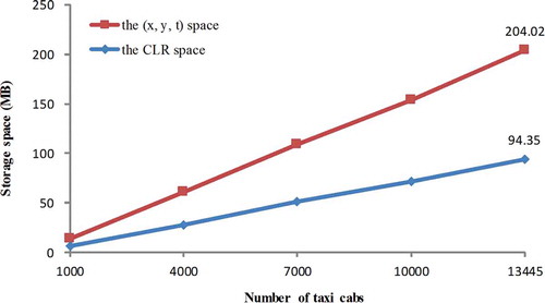
Figure 14 also shows the storage space required for storing the same floating car dataset in (x, y, t) space. It can be observed from the figure that the proposed spatiotemporal data model has a significant storage advantage over the classical data model. For example, the storage space required for storing space-time paths of 13,445 taxis in CLR space is approximately 46.2% of that required for storing the same dataset in (x, y, t) space. This result is expected for two reasons. First, the proposed spatiotemporal data model significantly reduces the number of control points required to store the space-time paths. To store space-time paths in classical (x, y, t) space, three types of control points are needed: GPS observations, network nodes, and link intermediate vertices. For example, 8,913,940 control points were used in (x, y, t) space to store 13,445 taxi space-time paths; and approximately 31% of these were link intermediate vertices. Using the proposed spatiotemporal data model in CLR space, the link intermediate vertex control points are no longer needed to maintain road geometry. Second, each control point is represented by two elements (i.e., z and t) in CLR space rather than three elements in (x, y, t) space, reducing storage space for each control point by 33%.

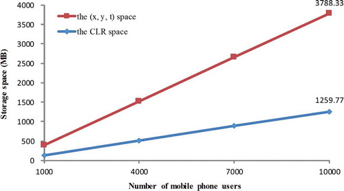
CLR space shows a significant storage advantage for the space-time prisms as well (see Figure 15). For example, storing space-time prisms of 10,000 mobile phone users in CLR space required 1259.77 MB, or 33% of the storage space required for the same dataset in (x, y, t) space. This storage efficiency is due to the same reasons as the space-time path case. For example, 82,757,434 control points at network nodes (49.88%) and link intermediate vertices (50.12%) were needed to store the space-time prisms of 10,000 users in (x, y, t) space, whereas only the first of these is needed in CLR space.

Figure 15. Storage space of space-time prisms.

5.3. Spatiotemporal query performance

This section examines the performance of the spatiotemporal queries presented in Section 4.3. All reported query performances were the average of 10 runs. Due to the lack of corresponding query implementation in (x, y, t) space in the literature, only queries in CLR space were examined. The query performance includes two components: the computational time for searching entities in the spatiotemporal indexes and the I/O time for retrieving the resultant spatiotemporal entities from the database. We cannot separate these two components, because we employed the ArcEngine development kit which integrates the components in the spatial query function. However, generally the first component is much smaller than the second.

Figure 16 shows the performance of the path-path intersection query: find all space-time paths of taxis intersecting the input path. To test the query performance under different numbers of taxis, five datasets were extracted from the original floating car dataset. The input path was the space-time path of a taxi randomly selected from the floating car dataset and used for all testing datasets. The performance degraded with the number of taxi cabs. For example, 0.71 seconds was required to perform a path-path intersection query in the dataset of 1000 taxis, whereas the query grew to 8.57 seconds for the full dataset with 13,445 taxis.

Figure 16. The path-path intersection query performance.

Figure 17 illustrates the performance of the window-path intersection query using the same five floating car datasets. The window-path intersection query is to find all space-time paths existing in the input spatial window W = (,,,) at any time instance during the input time period [,]. The query performance was examined in terms of three parameters: size of the spatial window, size of the time period, and the number of taxis in the dataset. The size of the input spatial window was measured by the number of network links intersecting the window. In all experiments, the starting time of the input time period was set as 8 a.m. and the length of time period was determined by the time interval. The performance of the window-path intersection query degraded with increase in taxi number in the dataset. However, the query performance is reasonable for this typical large-scale dataset of 13,445 taxis, requiring approximately 40 seconds when the size of spatial window was set to 10,000 links and time interval 60 minutes.

Figure 17. The window-path intersection query performance: (a) under different window sizes; (b) under different time intervals.

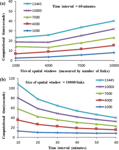
Figure 17(a) shows the computational performance of the window-path intersection query under different window sizes. The time interval was set to 60 minutes. The size of input spatial window has a significant impact on performance. For example, the window-path intersection query required 23 seconds on the dataset of 13,445 taxis with spatial window 1000 links, whereas this increases to approximately 40 seconds (1.73 times) when a spatial window of 10,000 links was used. This result was expected. The window-path intersection query employed a traditional spatial query on the Shenzhen road network to determine all links intersecting the input spatial window W. Then, a space-time region was constructed in CLR space by generating the set of space-time polygons for all the links . As with a traditional spatial query, the larger spatial window tended to require longer spatial query times. In addition, the more number of links intersecting the input spatial window, the more space-time polygons were generated to conduct the spatiotemporal query in CLR space, thus leading to the longer query time to find the space-time paths.

Figure 17(b) shows the computational time required by the window-path intersection query under different time intervals. The size of spatial window was set as 10,000 links. It is interesting that the performance improved with increasing time interval. For example, when the time interval was set 10 minutes, the query required approximately 108 seconds to the space-time paths on the dataset of 13,445 taxis, whereas when the time interval was increased to 60 minutes, the computational time significantly reduced by 63% to 40 seconds. This result may be due to the following reason. The input spatiotemporal window comprises a set of disjoin spatiotemporal polygons in CLR space. The increase of time interval would enlarge the sizes of spatiotemporal polygons, and increase the chance of spatiotemporal intersection with the taxi space-time paths. If the spatiotemporal intersection is determined between a spatiotemporal polygon and a taxi space-time path, then the spatiotemporal intersection relation will not be checked by the taxi space-time path with other spatiotemporal polygons of the input spatiotemporal window. Therefore, the increase of time interval would reduce the computational cost in determining the spatiotemporal intersection relation.

Figure 18 shows the performance of the station-prism within query and prism-prism intersection queries on the mobile phone tracking dataset. To test the performance of these two queries under different numbers of users, five datasets were extracted from the original dataset.

Figure 18. Computational performance of the station-prism within query and the prism-prism intersection query.

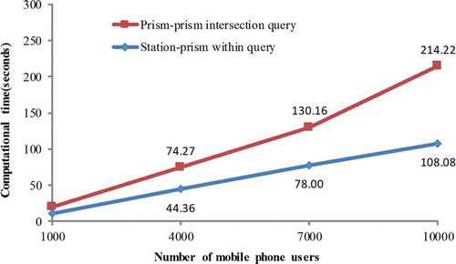
The station-prism within query was to find all mobile phone users feasible to conduct an activity at a given location during a time period [,]. A space-time station on the input location and time period was constructed and the spatiotemporal query was implemented as a spatial within query to find users’ space-time prisms containing the constructed station. The time period was set from 8:00 to 8:30 a.m. and the location was randomly selected from the set of POIs (points of interesting) in Shenzhen city. As shown in the figure, the performance of station-prism within query was reasonable for all five datasets. For example, the query required approximately 11 seconds for the dataset of 1000 users and 108 seconds for the dataset of 10,000 users.

The prism-prism intersection query was to find all mobile phone users feasible to conduct a joint activity with a given individual. Using the space-time prism of the given individual as the input, this spatiotemporal query was implemented as a spatial intersection query to find users’ space-time prisms intersecting the input prism. The input space-time prism was the space-time prism of a mobile phone user randomly selected from the mobile phone tracking dataset. As illustrated in Figure 18, the performance of prism-prism intersection query was reasonable for all five datasets. It required approximately 214 seconds for the dataset of 10,000 users. This spatiotemporal query required more computational time than the station-prism within query because the input space-time prism generally covered a large space-time region with several disjoint space-time polygons in CLR space.

6. Conclusions

This study proposed a spatiotemporal data model for time geographic entities and relations in road networks. The proposed spatiotemporal data model was built using the CLR technique. Network time geographic entities (including space-time path, station, prism, and lifeline) were transformed from 3D (x, y, t) space to 2D CLR space. The equivalence of representing network time geographic entities in CLR space and classical (x, y, t) space was rigorously proved. Space-time intersection relations were refined into five space-time sub-relations (i.e., Contains, Within, Touches, Overlaps, and Crosses) and implemented by the classical spatial topological relations in CLR space. Path bundling was formulated and solved as a space-time intersection problem using spatiotemporal buffering. Using the proposed spatiotemporal data model, four spatiotemporal queries were developed: path-path intersection query, window-path intersection query, station-prism within query, and prism-prism intersection query.

Compared with the classical data model in (x, y, t) space, the proposed spatiotemporal data model has several unique features.

1. Using the proposed spatiotemporal data model, the network time geographic entities can be stored and managed in classical spatial databases. This makes it easy to integrate time geographic analysis with the powerful visualization and spatial analysis capabilities provided by contemporary GIS platforms.

2. Numerous efficient spatial operations can be directly utilized to implement spatiotemporal operations for network time geographic entities in CLR space. This can lead to more efficient time geographic analysis, since it is always computationally simpler to manipulate entities in 2D space than 3D space.

3. Existing well-developed spatial index structures can be directly employed to implement spatiotemporal queries on the network time geographic entities in CLR space. This can lead to efficient spatiotemporal queries on large-scale time geographic datasets.

To validate the proposed spatiotemporal data model, a prototype system was implemented using the ArcGIS spatial database and development kit. A case study using real space-time paths of taxis and space-time prisms of mobile phone users was performed on the Shenzhen road network. The proposed model provides 54% and 67% storage space reductions for space-time paths and prisms, respectively, compared with the classical data model. Spatiotemporal queries on the prototype CLR space system showed reasonable performance for large-scale time geographic datasets.

Due to space limitations, the computational experiments presented in this article are by no means comprehensive. In the case study, the Grid-file index was employed and examined for the spatiotemporal queries of space-time paths and prisms. Other well-developed spatial indexes, such as R-tree and Quad-tree, can also be used as the spatiotemporal index in the CLR space. However, which spatial index techniques perform best in the CLR space needs further investigations. In the case study, the storage and query performances of space-time paths in the CLR space were examined using the ArcSDE and Oracle techniques. Comparing such performances of space-time paths with the existing moving objects databases techniques (De Almeida and Güting 2005, Güting et al. 2006) is required in the future studies.

Several directions for future research are worth noting. First, the proposed spatiotemporal data model has only been applied to time geographic entities in a single-mode road network. The extension to multi-mode networks (e.g., bus and subway) is an interesting topic for further work. The extension of the proposed model to the planar space, where people can move freely in the geographical space, also needs further studies. Second, ArcSDE and Oracle were adopted in the case study as the spatial database. The integration of emerging non-SQL database techniques (e.g., Mongo DB) may be a possible way to further improve the performance of spatiotemporal queries. Last but not least, this study presented four simple spatiotemporal queries for illustration, which clearly needs to be extended. The application of the proposed spatiotemporal data model for human mobility studies and advanced time geographic analysis is warranted for further study.

Acknowledgment

The authors are thankful to the anonymous referees for their comments and suggestions that improved this article.

Disclosure statement

No potential conflict of interest was reported by the authors.

Additional information

Funding

The work described in this article was jointly supported by research grants from the National Natural Science Foundation of China [grant number 41231171], [grant number 41571149], [grant number 41371377]; the Research Institute for Sustainable Urban Development (RISUD) of The Hong Kong Polytechnic University [grant number 1-ZVEW]; the Surveying & Mapping and Geoinformation Research in the Public Interest [201512026]; Shenzhen Scientific Research and Development Funding Program [grant number ZDSY20121019111146499]; and Shenzhen Dedicated Funding of Strategic Emerging Industry Development Program [grant number JCYJ20121019111128765].

References

- Armstrong, M.P., 1988. Temporality in spatial databases. In: Proceedings of GIS/LIS’88, San Antonio, TX. Bethesda, MD: American Society for Photogrammetry and Remote Sensing, 880–889.
- Charleux, L., 2015. A modification of the time-geographic framework to support temporal flexibility in ‘fixed’ activities. International Journal of Geographical Information Science, 29, 1125–1143. doi:10.1080/13658816.2015.1009464
- Chen, B.Y., et al., 2013. Reliable space-time prisms under travel time uncertainty. Annals of the Association of American Geographers, 103, 1502–1521. doi:10.1080/00045608.2013.834236
- Chen, B.Y., et al., 2012. Development of dynamic three-dimensional coastal information system: a case study in Hong Kong. Journal of Hydroinformatics, 14, 815–828. doi:10.2166/hydro.2012.048
- Chen, B.Y., et al. 2015. Space-time path bundling based on spatiotemporal buffering operations. Working paper.
- Chen, B.Y., et al., 2014. Map matching algorithm for large-scale low-frequency floating car data. International Journal of Geographical Information Science, 28, 22–38. doi:10.1080/13658816.2013.816427
- Chen, J., et al., 2011. Exploratory data analysis of activity diary data: a space-time GIS approach. Journal of Transport Geography, 19, 394–404. doi:10.1016/j.jtrangeo.2010.11.002
- De Almeida, V.T. and Güting, R.H., 2005. Indexing the trajectories of moving objects in networks. Geoinformatica, 9, 33–60. doi:10.1007/s10707-004-5621-7
- Egenhofer, M.D. and Herring, J., 1990. A mathematical framework for the definition of topological relationships. In: Proceedings of the fourth international symposium on spatial data handling. Zurich. Zurich: University of Zurich, 803–813.
- Erwig, M., et al., 1999. Spatio-temporal data types: an approach to modelling and querying moving objects in databases. GeoInformatica, 3, 269–296. doi:10.1023/A:1009805532638
- Fang, Z.X., et al., 2012. Spatiotemporal analysis of critical transportation links based on time geographic concepts: a case study of critical bridges in Wuhan, China. Journal of Transport Geography, 23, 44–59. doi:10.1016/j.jtrangeo.2012.03.018
- Fang, Z.X., et al., 2011. A multi-objective approach to scheduling joint participation with variable space and time preferences and opportunities. Journal of Transport Geography, 19, 623–634. doi:10.1016/j.jtrangeo.2010.06.019
- Finkel, R. and Bentley, J.L., 1974. Quad trees a data structure for retrieval on composite keys. Acta Informatica, 4, 1–9. doi:10.1007/BF00288933
- Goodchild, M.F., 2013. Prospects for a space-time GIS. Annals of the Association of American Geographers, 103, 1072–1077. doi:10.1080/00045608.2013.792175
- Goodchild, M.F., Yuan, M., and Cova, T.J., 2007. Towards a general theory of geographic representation in GIS. International Journal of Geographical Information Science, 21, 239–260. doi:10.1080/13658810600965271
- Güting, R.H., De Almeida, V.T., and Ding, Z.M., 2006. Modeling and querying moving objects in networks. The VLDB Journal, 15, 165–190. doi:10.1007/s00778-005-0152-x
- Güting, R.H. and Schneider, M., 2005. Moving objects databases. San Francisco: Morgan Kaufmann.
- Guttman, A., 1984. R-trees: a dynamic index structure for spatial searching. In: B. Yormark, ed. SIGMOD conference 1984, Boston, MA. New York, NY: ACM, 47–57.
- Hägerstrand, T., 1970. What about people in regional science? Papers in regional. Science, 24, 7–24.
- Herring, J., 2011, Open GIS implementation specification for geographic information - simple feature access - part 1: common architecture. Available from: http://www.opengeospatial.org/standards/sfa
- Huang, B. and Wu, Q., 2008. Dynamic accessibility analysis in location-based service using an incremental parallel algorithm. Environment and Planning B: Planning and Design, 35, 831–846. doi:10.1068/b33118
- Huang, B., Wu, Q., and Zhan, F.B., 2007. A shortest path algorithm with novel heuristics for dynamic transportation networks. International Journal of Geographical Information Science, 21, 625–644. doi:10.1080/13658810601079759
- Kuijpers, B. and Othman, W., 2009. Modeling uncertainty of moving objects on road networks via space-time prisms. International Journal of Geographical Information Science, 23, 1095–1117. doi:10.1080/13658810802097485
- Kwan, M.-P., 2000. Interactive geovisualization of activity-travel patterns using three-dimensional geographical information systems: a methodological exploration with a large data set. Transportation Research Part C: Emerging Technologies, 8, 185–203. doi:10.1016/S0968-090X(00)00017-6
- Kwan, M.-P., 2013. Beyond space (as we knew it): toward temporally integrated geographies of segregation, health, and accessibility. Annals of the Association of American Geographers, 103, 1078–1086. doi:10.1080/00045608.2013.792177
- Kwan, M.-P. and Neutens, T., 2014. Space-time research in GIScience. International Journal of Geographical Information Science, 28, 851–854. doi:10.1080/13658816.2014.889300
- Kwan, M.-P. and Weber, J., 2003. Individual accessibility revisited: implications for geographical analysis in the twenty-first century. Geographical Analysis, 35, 341–353. doi:10.1111/gean.2003.35.issue-4
- Langran, G. and Chrisman, N.R., 1988. A framework for temporal geographic information. Cartographica: The International Journal for Geographic Information and Geovisualization, 25, 1–14. doi:10.3138/K877-7273-2238-5Q6V
- Li, D., et al., 2013. Geomatics for smart cities: concept, key techniques, and applications. Geo-spatial Information Science, 16, 13–24. doi:10.1080/10095020.2013.772803
- Li, Q.Q., et al., 2015. A hybrid link-node approach for finding shortest paths in road networks with turn restrictions. Transactions in GIS. doi:10.1111/tgis.12133
- Li, X. and Lin, H., 2006. Indexing network-constrained trajectories for connectivity-based queries. International Journal of Geographical Information Science, 20, 303–328. doi:10.1080/13658810500432570
- Long, J.A. and Nelson, T.A., 2013. A review of quantitative methods for movement data. International Journal of Geographical Information Science, 27, 292–318. doi:10.1080/13658816.2012.682578
- Miller, H.J., 1991. Modelling accessibility using space-time prism concepts within geographical information systems. International Journal of Geographical Information Systems, 5, 287–301. doi:10.1080/02693799108927856
- Miller, H.J., 2005. A measurement theory for time geography. Geographical Analysis, 37, 17–45. doi:10.1111/gean.2005.37.issue-1
- Miller, H.J. and Bridwell, S.A., 2009. A field-based theory for time geography. Annals of the Association of American Geographers, 99, 49–75. doi:10.1080/00045600802471049
- Miller, H.J. and Shaw, S.L., 2001. Geographic information systems for transportation: principles and applications. New York: Oxford University Press.
- Nakaya, T., 2013. Analytical data transformations in space-time region: three stories of space-time cube. Annals of the Association of American Geographers, 103, 1100–1106. doi:10.1080/00045608.2013.792184
- Neutens, T., et al., 2008. A three-dimensional network-based space-time prism. Journal of Geographical Systems, 10, 89–107. doi:10.1007/s10109-007-0057-x
- Nievergelt, J., Hinterberger, H., and Sevcik, K.C., 1984. The grid file: an adaptable, symmetric multikey file structure. ACM Transactions on Database Systems, 9, 38–71. doi:10.1145/348.318586
- Pei, T., et al., 2014. A new insight into land use classification based on aggregated mobile phone data. International Journal of Geographical Information Science, 28, 1988–2007. doi:10.1080/13658816.2014.913794
- Peuquet, D.J. and Duan, N., 1995. An event-based spatiotemporal data model (ESTDM) for temporal analysis of geographical data. International Journal of Geographical Information Systems, 9, 7–24. doi:10.1080/02693799508902022
- Popa, I.S., et al., 2015. Spatio-temporal compression of trajectories in road networks. Geoinformatica, 19, 117–145. doi:10.1007/s10707-014-0208-4
- Richardson, D.B., et al., 2013. Spatial turn in health research. Science, 339, 1390–1392. doi:10.1126/science.1232257
- Shaw, S.-L. and Yu, H.B., 2009. A GIS-based time-geographic approach of studying individual activities and interactions in a hybrid physical-virtual space. Journal of Transport Geography, 17, 141–149. doi:10.1016/j.jtrangeo.2008.11.012
- Song, C.M., et al., 2010. Limits of predictability in human mobility. Science, 327, 1018–1021. doi:10.1126/science.1177170
- Versichele, M., et al., 2014. Time-geographic derivation of feasible co-presence opportunities from network-constrained episodic movement data. Transactions in GIS, 18, 687–703. doi:10.1111/tgis.2014.18.issue-5
- Wang, D.G. and Cheng, T., 2001. A spatio-temporal data model for activity-based transport demand modelling. International Journal of Geographical Information Science, 15, 561–585. doi:10.1080/13658810110046934
- Wolfson, O., et al., 1998. Moving object databases: issues and solutions. In: Proceedings of the 10th international conference on scientific and statistical database management, Capri. New York, NY: IEEE, 111–122.
- Xu, J.Q. and Güting, R.H., 2013. A generic data model for moving objects. Geoinformatica, 17, 125–172. doi:10.1007/s10707-012-0158-7
- Yu, H. and Shaw, S.-L., 2008. Exploring potential human activities in physical and virtual spaces: a spatio-temporal GIS approach. International Journal of Geographical Information Science, 22, 409–430. doi:10.1080/13658810701427569
- Yuan, M., 1999. Use of a three-domain representation to enhance GIS support for complex spatiotemporal queries. Transactions in GIS, 3, 137–159. doi:10.1111/1467-9671.00012
- Yue, Y., et al., 2014. Zooming into individuals to understand the collective: a review of trajectory-based travel behaviour studies. Travel Behaviour and Society, 1, 69–78. doi:10.1016/j.tbs.2013.12.002