A spatial and statistical analysis of the impact of transformation of raster cost surfaces on the variation of least-cost paths

ABSTRACT

Planners who are involved in locational decision-making often use raster-based geographic information systems to quantify the value of land in terms of suitability or cost for a certain use. From a computational point of view, this process can be seen as a transformation of one or more sets of values associated with a grid of cells into another set of such values through a function reflecting one or more criteria. While it is generally anticipated that different transformations lead to different ‘best’ locations, little has been known on how such differences arise (or do not arise). The paper attempts to answer this question in the context of path planning through a series of computational experiments using a number of random landscape grids with a variety of spatial and nonspatial structures. In the experiments, we generated least-cost paths on a number of cost grids transformed from the landscape grids using a variety of transformation parameters and analyzed the locations and (weighted) lengths of those paths. Results show that the same pair of terminal cells may well be connected by different least-cost paths on different cost grids though derived from the same landscape grid and that the variation among those paths is affected by how given values are distributed in the landscape grid as well as by how derived values are distributed in the cost grids. Most significantly, the variation tends to be smaller when the landscape grid contains more distinct patches of cells potentially attracting or distracting cost-saving passage or when the cost grid contains a smaller number of low-cost cells.

KEYWORDS:

• Least-cost paths
• raster cost surfaces
• land evaluation
• suitability analysis
• spatial decision support

1. Introduction

Selection of a suitable site for a target use is an important locational decision problem in planning. If the study area is effectively discretized into a grid of cells, the problem can be cast as one of combining one or more cells into a group that best fits the use as a whole. Combinatorial optimization models and algorithms have been developed for and applied to a variety of such problems and often facilitated by being integrated into raster-based geographic information systems (GIS) (see Malczewski (2006) for a survey). Some of them pertain to sites of areal form represented by regions of cells (e.g. Brookes 1997, Cova and Church 2000, Williams 2002, Shirabe 2005, 2011, Xiao 2006, Duque et al. (2007), for a review) and others to sites of linear form represented by sequences of cells (e.g. Goodchild 1977, Huber and Church 1985, Douglas 1994, Xu and Lathrop 1995, Collischonn and Pilar 2000, Tomlin 2010, Antikainen (2013), for a review) or by swaths of cells (Gonçalves 2010, Shirabe 2016).

Site selection is often preceded by land evaluation, which estimates the degree of positive or negative impact – which may be generally referred to as ‘suitability’ or ‘cost’, respectively – of each unit of land being used for the use of interest. This requires a good understanding and interpretation of the underlying ecological processes and involves manipulation and integration of a large volume of environmental and social data, as well illustrated by the pioneering work of McHarg (1969).

The data processing aspect of land evaluation can be facilitated by raster-based GIS, which represent a given landscape with one or more variables (or factors or attributes) each assigning a single value to each cell of the reference grid. In particular, the map algebraic capabilities available in many existing GIS (Tomlin 1990, 1994) are useful in two related tasks: 1) scoring, for each cell, a suitability or cost value with respect to each relevant variable and 2) aggregating, for each cell, all such values into a composite value.

The latter task may be done through a ‘(weighted) linear combination’ (Hopkins 1977, Eastman et al. 1998) or ‘weighted summation’ (Jankowski 1995) in which two or more values of each cell are multiplied by weights reflecting their relative importance before being summed. This mechanism is easy to understand and implement but involves uncertainty and subjectivity in determination of the weights (see, e.g. Lai and Hopkins 1989, Hobbs et al. 1992, Malczewski 2000, Basnet et al. 2001, Ligmann-Zielinska and Jankowski 2014), which is problematic since different sets of weights can easily lead to different solutions (see Atkinson et al. (2005), Choi et al. (2009), and Bagli et al. (2011) for case studies).

The effect of the former task on locational decision-making should not be overlooked, either, since one landscape variable can be, in theory, transformed in infinitely many different ways. Basnet and Apan (2007) experimentally demonstrated in the context of suitability analysis that the choice of transformation parameters such as classification method, class number, and value range can change the distribution of suitability values substantially. Of course, this does not necessarily mean that the selection of an optimal set of cells – optimal, i.e. maximizing the total suitability values or minimizing the total cost values – would be affected, too. Case studies are available in the literature (e.g. Larkin et al. 2004, Schadt et al. 2002, Driezen et al. 2007, Gonzales and Gergel 2007) that compared least-cost paths generated over cost grids with different ranges of values transformed from a land cover grid. Some of them found the locations and lengths of least-cost paths sensitive to the range of cost values, but others did not. The mixed results may reflect the reliance of each case study on one specific study area, whose landscape might have a special structure. An exception is Rayfield et al. (2010), who conducted a similar yet more systematic sensitivity analysis using 2000 randomly generated artificial raster landscapes and found that least-cost paths tend to deviate more from straight lines, even more so in fragmented landscapes, as the relative differences in the underlying cost values become larger.

In those studies whose primary focus was the range of cost values, the transformation of a landscape grid into a cost grid was justifiably limited to one-to-one correspondence, that is, each value in the input grid corresponds to exactly one value in the output grid and vice versa. In practice, however, more complex functions may be used and, intentionally or not, change the number of unique values and the number of cells for each value, which we suspect is another source of variation among potential least-cost paths.

To see this, consider a hypothetical planning problem of where to build a road to connect two terminuses in a study area in Rwanda, which is referenced to a 204-by-189 grid with a cell size of 10 m. To avoid the weighting problem mentioned earlier, suppose that the ideal location of the road minimizes the total cost associated with its construction, operation, maintenance, or any other activity and that the cost per unit length varies only with slope, whose values range from 0% to 127% and are highly autocorrelated (Moran’s I = 0.942) across the study area (indicated by shades in Figure 1(a)). Since no exact quantitative relationship is known between the two variables, we first take the opinion of a local expert suggesting that all cells be classified into three classes of an equal interval of slope values and that cost values of 1, 5 and 9 be assigned to the cells in the first, the second and the third (steepest) classes, respectively. Other experts, however, may well have different opinions and question the rationale for her choice of the classification method, the number of classes, or the range of cost values. This potential disagreement leads us to try all combinations of four different classification methods (i.e. equal interval, quantile, natural break and customized¹), three different numbers of classes (i.e. 3, 5 and 9), and two different ranges (i.e. 1–9 and 1–81). The resulting 24 cost grids have different distributions of cost values, over which the two terminuses are connected by different least-cost paths (see Figure 1(a)).

Figure 1. Variations of least-cost paths in two different areas. Each of (a) and (b) superimposes 24 least-cost paths (sequences of darkly shaded cells) between two cells (one near the upper left corner and the other near the lower right corner) on different cost grids (not shown) transformed from their common slope grid (on which darker shades represent steeper slopes).

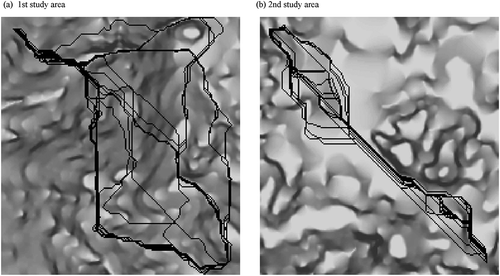
Now imagine that we are assigned another study area, which is 40 km apart from the first study area but has exactly the same spatial extent and resolution (204-by-189 grid with a cell size of 10 m) and a similar range (0–134%) and autocorrelation (Moran’s I = 0.950) of slope values (represented by shades in Figure 1(b)). Then let us apply to this second study area the same procedure described above and obtain another set of 24 least-cost paths, which look more clustering as seen in Figure 1(b). The variation in location of a set of paths may be quantified by the average number of paths intersected at each cell in the set, which is referred to here as ‘the number of paths per cell’ (or PPC for short) and ranges from 1 (indicating the highest variation) to 24 (indicating the lowest variation) in the present example. The 24 least-cost paths in the first case have a PPC of 2.27 and those in the second case have a PPC of 2.77, which implies that the former are more varying than the latter. Note that PPC is employed here for ease of computation and alternative measures may be admittedly preferred in other cases that take into account distance rather than intersection relationships between paths. One such alternative may measure the ‘Hausdorff distance’ (see Min et al. 2007 for a discussion in the context of GIS) between each path and the straight line between its ends, i.e. the distance of the farthest cell in that path from that line.

Just because paths are located at different locations, it does not mean that their lengths, whether Euclidean or weighted, are different, too. If the variation in length of a set of paths is measured by the coefficient of variation (CV) (i.e. the standard deviation divided by the mean) of the weighed lengths of those paths – weighted, i.e. with their common grid (representing percent slope in the present example), then we must say that the paths in the first case are less varying than those in the second case because their CVs are 0.084 and 0.216, respectively.

The variation of the 24 least-cost paths in each of the two cases, though to different extents, may be ascribed to the fact that their cost grids were simply different, although derived from the same slope grid. However, the difference was made deliberately in exactly the same way in both cases and thus does not explain why the paths in the first case were more varying in location and less varying in length. Did it happen merely by chance? Or are there any factors that at least partially account for it?

Through systematic computational experiments, the present work attempts to advance the knowledge on the inconsistency of least-cost paths due to the uncertainty of selected cost evaluation parameters. We have hypothesized that the degree of variability of least-cost paths is affected by both the way input landscape values are distributed (which are given to the land evaluator) and the way output cost values are distributed (which are to be controlled, directly or indirectly, by the land evaluator).

The remainder of the paper is structured as follows. Section 2 describes the details of the experiments in terms of how data were collected, processed and analyzed. Section 3 reports results of the experiments. Section 4 concludes the paper with a summary of major findings and implications of the results.

2. Method

We conducted four independent experiments using artificial landscape data. The first two experiments (Experiments 1 and 2) were similarly designed to study the variation of least-cost paths due to the difference in the shapes of frequency distribution of cell values in their cost grids. The last two experiments (Experiments 3 and 4), too, were designed similarly to each other, but for the study of the variation of least-cost paths due to the difference in the granularities and ranges of cell values in their cost grids.

Each pair of experiments examined nonspatial and spatial aspects of landscape grids separately as additional sources of variation of least-cost paths. In Experiment 1 (and Experiment 3), we were interested in whether the variation of least-cost paths on different cost grids derived from the same landscape grid is related to the shape of frequency distribution of cell values in the landscape grid. Experiments 2 (and Experiment 4) focused on the possible relationship of the variation of least-cost paths to the spatial structure of the landscape grid.

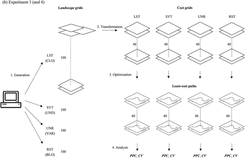
All four experiments had different purposes or focuses but were similar in their procedures, each involving four major steps. The first step was to generate a number of grids simulating various landscape variables. Second, each of the landscape grids was transformed into multiple cost grids reflecting various assumptions that actual land evaluators might have. Third, a least-cost path was delineated from each of the cost grids. Finally, all the least-cost paths were analyzed to find how (much) they varied and what factors might contribute to the variation. The flow of these steps is schematically illustrated in Figure 2 and the details of each step are explained below.

Figure 2. Flow of the four steps in (a) Experiment 1 (and 2) and (b) Experiment 3 (and 4). Four sets of landscape grids were initially generated, each set having an associated shape of frequency distribution (LST, SYT, UNR, or RST) in Experiments 1 and 3 or an associated pattern of spatial structure (CLO, UND, VAR, BLO) in Experiments in 2 and 4.

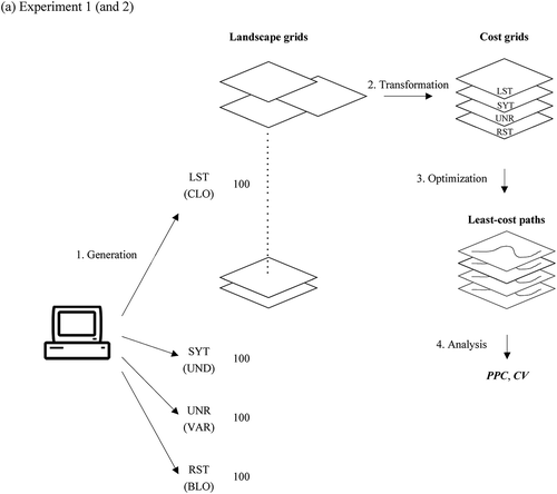
Figure 2. (Continued).

2.1. Generation of landscape grids

Each experiment used a different set of 400 grids with a size of 200×200 cells whose values were integers ranging from 1 to 100 with an increment of 1. All the grids had the same spatial extent and resolution and the same attribute range and granularity.

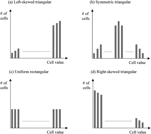
The landscape grids generated in Experiments 1 and 3 were populated with values in different shapes of frequency distribution with different degrees of autocorrelation. As illustrated in Figure 3, we considered four general shapes of frequency distribution including left-skewed triangular (LST), symmetric triangular (SYT), uniform rectangular (UNR) and right-skewed triangular (RST). Note that the number of low-value cells increases in this order.

Figure 3. Four shapes of frequency distributions of cell values: left-skewed triangular (LST), symmetric triangular (SYT), uniform rectangular (UNR) and right-skewed triangular (RST). Each shape is illustrated by a partial histogram in which the horizontal and vertical axes represent cell values and their frequencies, respectively, in a grid.

For each shape of frequency distribution, we performed the following procedure 100 times.

1. Assign each cell in a 200-by-200 grid an integer randomly chosen from 1 to 100 with an equal probability.

2. Smooth the grid by calculating for each cell the mean of all values within a randomly chosen integer radius ranging from 0 to 20 cell sides long from that cell. Note that in this calculation, the grid is regarded as a two-dimensional torus such that its first row is adjacent to its last row and its first column is adjacent to its last column so that discontinuities on those boundaries can be eliminated.

3. Classify the resulting values into 100 classes so that the number of cells in each class is consistent with the specified shape of frequency distribution.

4. Re-assign each cell an integer, which also ranges from 1 to 100, according to the order of its class.

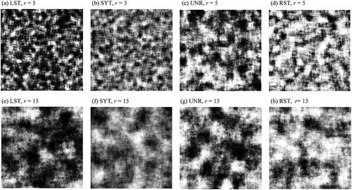
As a result, for each of the four shapes of frequency distribution, we obtained 100 random landscape grids – which look somewhat like clouds as shown in Figure 4 – each with its values spatially autocorrelated to a degree that increases with the smoothing radius.

Figure 4. Examples of landscape grids. Those on the same row have the same smoothing radius r = 5 or 15. Those on the same column have the same shape of frequency distribution, which is left-skewed triangular (LST), symmetric triangular (SYT), uniform rectangular (UNR), or right-skewed triangular (RST). The darker shades represent higher values.

In each of Experiments 2 and 4, four sets of 100 random landscape grids were generated and one of the following four patterns of spatial structure was uniquely associated with each set: ‘cloudy (CLO)’, ‘undulating (UND)’, ‘variegated (VAR)’ and ‘blobby (BLO)’. The values of the cells in all the grids were distributed in the UNR shape of frequency distribution as well as in the pattern of spatial structure associated with the set to which those grids belonged.

Each cloudy landscape grid (see Figure 5(a) for an example) was generated with the same procedure described above but with the smoothing radius set to 10 in Step 2 and with the shape of frequency distribution set to UNR in Step 3. Each undulating landscape grid (see Figure 5(b) for an example) was generated using the following procedure.

1. Assign each cell in a single row of 200 cells an integer randomly chosen from 1 to 100 with an equal probability.

2. Smooth the row twice, each time by calculating for each cell the mean of all values within a distance of 10 cell sides long from that cell. Note that in this calculation, the row is regarded as a one-dimensional torus such that its first cell is adjacent to its last cell.

3. Classify the resulting values into 100 classes so that each class contains the same number of cells.

4. Re-assign each cell an integer, which also ranges from 1 to 100, according to the order of its class.

5. Make 199 copies of the row, and vertically append all 200 identical rows (including the original) one after another in a way that each row is shifted randomly to the left, to the right, or neither from its previous row.

6. Cut the segment of each row if it exceeds the boundary of the first row on either side and paste it to the opposite side of that row to make the result a 200-by-200 grid.

Figure 5. Examples of landscape grids with four different patterns of spatial structure: (a) cloudy (CLO), (b) undulating (UND), (c) variegated (VAR) and (d) blobby (BLO). The darker shades represent higher values. Note that all grids contain 400 cells for each integer value from 1 to 100.

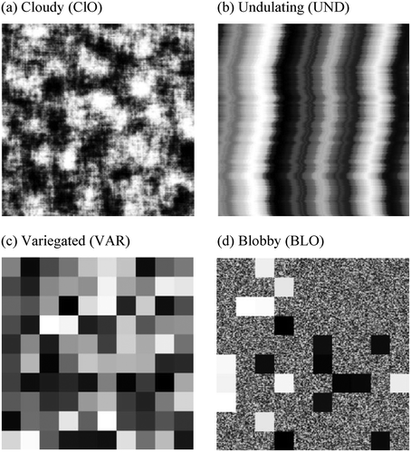
Each variegated landscape grid (see Figure 5(c) for an example) was generated by dividing the 200-by-200 grid into 100 20-by-20 square patches and assigning each patch an integer randomly chosen from 1 to 100 without repetition. Each blobby landscape grid (see Figure 5(d) for an example) was generated by first dividing the 200-by-200 grid into 100 20-by-20 square patches, then assigning the lowest 10 values (i.e. 1–10) and the highest 10 values (i.e. 91–100) to 20 randomly selected patches, and finally assigning each of the middle 80 values (i.e. 11–90) to 400 cells randomly selected from the rest of the grid.

While we tried to ensure that our synthetic data represent diverse configurations of a plurality of landscape features in mutually related manners, we must acknowledge that actual landscapes involve more complex processes than our simulations.

2.2. Transformation of landscape grids into cost grids

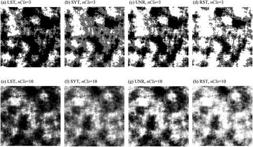
In Experiments 1 and 2, we transformed each of the 400 landscape grids into four cost grids with a common range and granularity but different shapes (i.e. LST, SYT, UNR and RST) of distribution of cell values. The range started with 1 and ended with an integer, max, randomly chosen from 10, 20, 40, 80 and 160 with an equal probability. The granularity was measured in terms of number of classes, nCls, which was randomly chosen from 3, 4, 5, 6, 7, 8, 9 and 10 with an equal probability. For example, if a landscape grid is transformed into four cost grids with max = 40 and nCls = 5, the one with a LST distribution will have 2667 cells of the value of 1, 5333 cells of the value of 11, 8000 cells of the value of 21, 10667 cells of the value of 31, and 13333 cells of the value of 40. Figure 6 illustrates examples of cost grids.

Figure 6. Examples of cost grids. Those on the same row have the same number of classes nCls = 3 or 10, and were derived from the same landscape grid but have different shapes of frequency distribution, i.e. left-skewed triangular (LST), symmetric triangular (SYT), uniform rectangular (UNR) and right-skewed triangular (RST). The darker shades represent higher values.

In Experiments 3 and 4, we transformed each of the 400 landscape grids into 160 cost grids – one for each combination of a shape of frequency distribution (i.e. LST, SYT, UNR or RST), a max value (i.e. 10, 20, 40, 80 or 160), and a nCls value (i.e. 3, 4, 5, 6, 7, 8, 9 or 10) – in the same manner as in Experiments 1 and 2.

It is important to note that, when a land evaluator transforms a landscape grid into a cost grid in practice, the landscape grid is assumed to be a fact and the cost grid is an interpretation of it reflecting the land evaluator’s intention and assumption. In some cases, the land evaluator has a direct control over the shape of the frequency distribution of cell values in the cost grid. For instance, if a quantile classification is used, the cell values in the cost grid will be distributed uniformly, regardless of how those in the landscape grid are originally distributed. Another example is an equal-interval classification, which will give the cost grid the same shape of frequency distribution as the landscape grid. In other cases, the land evaluator takes a more passive role in shaping the frequency distribution of cell values in the cost grid. For instance, if the transformation is done using a classification method that defines ‘natural breaks’ (Jenks 1967) between classes or an application-specific formula that simulates the underlying ecological process, then the shape of distribution of output values cannot be specified in advance.

2.3 Delineation of least-cost paths

In all four experiments, we delineated a least-cost path between two terminal cells on each of the cost grids generated in the previous step. The terminal cells were fixed throughout at the 10th row and 10th column from the upper left corner of the 200-by-200 grid and at the 10th row and 10th column from the lower right corner.

2.4 Analysis of least-cost paths

In Experiment 1, four least-cost paths were generated from each landscape grid. To evaluate their variation in terms both of location and of weighted length, we calculated their PPC and CV (as defined in Section 1), respectively, where the length of each of the four paths was calculated based on their common landscape grid, i.e. as the sum of the Euclidean distance between each successive two cells in the path multiplied by their average cell value on that landscape grid. As a result, we obtained four samples of 100 PPCs and 100 CVs, one sample for each of the LST, SYT, UNR and RST shapes of frequency distribution considered for landscape grids. They were referred to as LST, SYT, UNR and RST samples accordingly. Then we conducted a series of statistical tests to see whether PPC or CV varies with the shape of frequency distribution of its associated landscape grid. Also, we regressed both PPC and CV against the smoothing radius, r, of the landscape grid and max and nCls of the cost grid separately to see if they are related to any of those variables.

In Experiment 2, we obtained four samples of 100 PPCs and 100 CVs and analyzed them in the same manner as those in Experiment 1. The four samples were associated with the CLO, UND, VAR and BLO patterns of spatial structure considered for landscape grids and thus referred to as the CLO, UND, VAR and BLO samples.

In Experiment 3, for each landscape grid, 160 least-cost paths were generated, which were divided into four groups of 40 least-cost paths, one group for each shape of frequency distribution considered for cost grids. We calculated each group’s PPC and CV. As a result, we obtained 16 samples of 100 PPCs and 100 CVs, one sample for each combination of two shapes of frequency distribution, one considered for landscape grids and the other for cost grids. They were referred to as the LST-LST, -SYT, -UNR and -RST, SYT-LST, -SYT, -UNR and -RST, UNR-LST, -SYT, -UNR and -RST, and RST-LST, -SYT, -UNR and -RST samples accordingly. We conducted statistical tests for whether PPC or CV varies with the shape of frequency distribution of its associated landscape grid or with that of its associated cost grids. Also we regressed both PPC and CV against r for possible relationships.

In Experiment 4, we obtained 16 samples of 100 PPCs and 100 CVs and analyzed them in the same manner as those in Experiment 3. The 16 samples were associated with all combinations of one of the four patterns of spatial structure considered for landscape grids and one of the four shapes of frequency distribution considered for cost grids and thus referred to as the CLO-LST, -SYT, -UNR and -RST, UND-LST, -SYT, -UNR and -RST, VAR-LST, -SYT, -UNR and – RST, and BLO-LST, -SYT, -UNR and -RST samples.

3. Results

Results of the four experiments are presented below. Keep in mind throughout that a larger PPC or a smaller CV indicate less variation of least-cost paths in location and in weighted length, respectively.

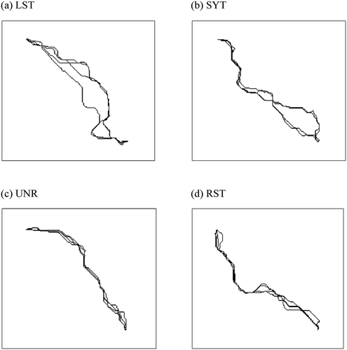
3.1. Experiment 1

Whichever sample it was taken from, every group of four-least cost paths exhibited discernable variation (see Figure 7 for an example from each sample) but it was hard to tell if any sample had a unique trend only by visual inspection. In fact, as seen in Table 1(a), all four samples have similar mean PPCs and mean CVs. Two-tailed t-tests also supported that there is no statistically significant difference in mean PPC or mean CV between any two samples. Note that we adopted the 5% level of significance for this and all other statistical tests we performed.

Table 1. Results of Experiment 1.

(a) Mean PPC and mean CV of four least-cost paths
Sample	Mean PPC	Mean CV
LST	1.4664	0.0761
SYT	1.4537	0.0737
UNR	1.4379	0.0738
RST	1.4659	0.0711
(b) Regression of PPC against r, max and nCls
Sample	r	max	nCls
LST	[−0.03273, −0.01859] 1.23*10^−10 0.3460	[−0.00196, 0.00030] 0.150 0.0210	[0.03681, 0.08206] 1.03*10^−6 0.2171
SYT	[−0.01632, −0.00337] 3.23*10^−3 0.0851	[−0.00140, 0.00013] 0.0542 0.0373	[0.03305, 0.06197] 3.07*10^−9 0.3026
UNR	[−0.02436, −0.00948] 1.77*10^−5 0.1722	[−0.00104, 0.00070] 0.699 0.0015	[0.04261, 0.07658] 3.82*10^−10 0.3310
RST	[−0.02422, −0.00974] 1.02*10^−5 0.1809	[−0.00143, 0.00025] 0.164 0.0197	[0.03465, 0.07314] 2.37*10^−7 0.2396
(c) Regression of CV against r, max and nCls
Sample	r	max	nCls
LST	[−0.00026, 0.00191] 0.135 0.0226	[0.00013, 0.00040] 1.51*10^−4 0.1369	[−0.00874, −0.00274] 2.52*10^−4 0.1284
SYT	[−0.00176, 0.00085] 0.490 0.0049	[0.00023, 0.00047] 7.52*10^−8 0.2567	[−0.00781, −0.00139] 5.48*10^−3 0.0761
UNR	[−0.00133, 0.00171] 0.801 6.50*10^−4	[0.00003, 0.00035] 0.0178 0.0560	[−0.01365, −0.00715] 6.64*10^−9 0.2917
RST	[−0.00104, 0.00193] 0.553 0.0036	[0.00004, 0.00034] 0.0144 0.0596	[−0.01601, −0.00963] 2.86*10^−12 0.3936

Note that each cell in (b) and (c) contains the 95% confidence interval (CI), p-value, coefficient of determination (r²) in this order for the corresponding regressor.

Figure 7. Examples of groups of four least-cost paths in Experiment 1. One group was taken from each of the (a) LST, (b) SYT, (c) UNR and (d) RST samples.

Table 1(b) and (c) summarize results of the regression analysis, which generally suggest that PPC and CV have positive and negative linear relationships, respectively, with nCls. Both relationships are statistically significant and moderate. For instance, according to the regression coefficient (or slope) of CV against nCls obtained from the LST sample, the maximum change in nCls (from 3 to 10 or vice versa) would change the mean CV by a value between 0.0192 (= 0.00274∙7) and 0.0612 (= 0.00874∙7). The relationships of PPC and CV with the two other variables are, however, quite different from each other. PPC has a statistically significant (moderate, negative) linear relationship with r, but not with max. CV, on the other hand, has a statistically significant (weak, positive) linear relationship with max, but not with r.

3.2. Experiment 2

It can be found in Table 2(a) that the mean PPC and the mean CV increases and decreases, respectively, in the order of the UND, CLO, BLO and VAR samples, although two-tailed t-tests did not find a statistically significant difference in the mean CV between the UND and CLO samples or between the BLO and VAR samples. This suggests that both PPC and CV are affected by the pattern of spatial structure of their associated landscape grid.

Table 2. Results of Experiment 2.

(a) Mean PPC and mean CV of four least-cost paths
Sample	Mean PPC	Mean CV
UND	1.2570	0.0854
CLO	1.3977	0.0844
BLO	1.6381	0.0397
VAR	2.0679	0.0389
(b) Regression of PPC against max and nCls
Sample	max	nCls
UND	[−0.00025, 0.00056] 0.439 0.0061	[0.00901, 0.02786] 1.90*10^−4 0.1331
CLO	[−0.00134, −0.00003] 0.040 0.0421	[0.04895, 0.07132] 4.28*10^−18 0.5374
BLO	[−0.00048, 0.00145] 0.321 0.0101	[0.04267, 0.08949] 1.95*10^−7 0.2425
VAR	[−0.00410, −0.00062] 8.20*10^−3 0.0692	[0.05792, 0.13994] 6.00*10^−6 0.1895
(c) Regression of CV against max and nCls
Sample	max	nCls
UND	[−0.00004, 0.00018] 0.187 0.0177	[−0.00702, −0.00179] 1.19*10^−3 0.1022
CLO	[0.00006, 0.00037] 7.63*10^−3 0.0704	[−0.01543, −0.00913] 9.01*10^−12 0.3795
BLO	[0.00013, 0.00033] 1.78*10^−5 0.1720	[−0.01144, −0.00657] 6.46*10^−11 0.3544
VAR	[−0.00006, 0.00017] 0.325 0.0099	[−0.00852, −0.00309] 4.93*10^−5 0.1554

Note that each cell in (b) and (c) contains the 95% confidence interval (CI), p-value, coefficient of determination (r²) in this order for the corresponding regressor.

Results of the regression analysis reported in Table 2(b) and (c) indicate that both PPC and CV have a statistically significant, moderate linear relationship with nCls, regardless of the pattern of spatial structure of their associated landscape grid. On the contrary, their relationships with max are generally (except for CV in the BLO sample) either statistically insignificant, weak, or dominated by other factors as indicated by small p-values, gentle regression slopes, or low coefficients of determination, respectively.

3.3. Experiment 3

As was the case with the preceding experiments, we saw some variation in every group of 40 least-cost paths (see Figure 8 for an example from each sample). There might be different trends in different samples, but they were at least not visually detectable.

Figure 8. Examples of groups of 40 least-cost paths in Experiment 3. One group is taken from each of the 16 samples (from (a) LST-LST to (p) RST-RST).

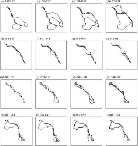
Table 3(a) and (b) show the mean PPCs and the mean CVs of all 16 samples, respectively. A trend can be seen that the mean PPC decreases and the mean CV increases from left to right (i.e. in the order of LST, SYT, UNR and RST columns), except that there is no statistically significant difference in PPC between the SYT and UNR columns. This implies that both PPC and CV vary with the shape of frequency distribution of the cost grids on which the paths are generated. As far as CV is concerned, this tendency is sensitive to the shape of frequency distribution of the landscape grid from which those cost grids are derived. With reference to Table 3(b), the ranges of mean CVs in the LST and SYT rows (i.e. [0.0488, 0.0958] and [0.0485, 0.0996], respectively) are much narrower than those the UNR and RST rows (i.e. [0.0376, 0.1331] and [0.0409, 0.1366], respectively). This is not the case with PPC.

Table 3. Results of Experiment 3.

Sample	LST	SYT	UNR	RST
(a) Mean PPC of 40 least-cost paths
LST	9.8474	8.3432	8.4254	6.5145
SYT	10.1664	8.5993	8.8065	6.5392
UNR	10.1990	8.4461	8.7451	6.5330
RST	10.3037	8.5582	8.5461	6.3545
(b) Mean CV of 40 least-cost paths
LST	0.0488	0.0699	0.0817	0.0958
SYT	0.0485	0.0662	0.0781	0.0996
UNR	0.0376	0.0612	0.0920	0.1331
RST	0.0409	0.0614	0.0909	0.1366
(c) Regression of PPC against r
LST	[−0.24763, −0.12535] 2.61*10^−8 0.2722	[−0.22291, −0.10188] 6.4*10^−7 0.2244	[−0.17482, −0.06862] 1.54*10^−5 0.1744	[−0.11383, −0.02653] 1.91*10^−3 0.0941
SYT	[−0.30611, −0.16959] 4.81*10^−10 0.3279	[−0.24464, −0.12911] 4.88*10^−9 0.2961	[−0.22862, −0.10119] 1.42*10^−6 0.2121	[−0.10146, −0.00659] 0.0260 0.0496
UNR	[−0.24449, −0.11284] 4.94*10^−7 0.2284	[−0.19334, −0.08267] 3.09*10^−6 0.2000	[−0.20249, −0.07285] 5.57*10^−5 0.1534	[−0.08644, −0.00570] 0.0257 0.0497
RST	[−0.33326, −0.17346] 8.79*10^−9 0.2878	[−0.23338, −0.11296] 1.22*10^−7 0.2495	[−0.17689, −0.04321] 1.50*10^−3 0.0982	[−0.06402, 0.02375] 0.365 0.0084
(d) Regression of CV against r
LST	[−0.00037, 0.00070] 0.544 0.0038	[−0.00073, 0.00076] 0.965 1.99*10^−5	[−0.00165, 0.00035] 0.198 0.0168	[−0.00204, 0.00057] 0.268 0.0125
SYT	[−0.00015, 0.00101] 0.141 0.0220	[−0.00075, 0.00071] 0.956 3.14*10^−5	[−0.00178, 0.00049] 0.260 0.0129	[−0.00240, 0.00037] 0.147 0.0213
UNR	[0.00023, 0.00102] 24.3*10^−3 0.0900	[0.00003, 0.00120] 0.0382 0.0431	[−0.00065, 0.00118] 0.569 0.0033	[−0.00171, 0.00084] 0.502 0.0046
RST	[0.00001, 0.00087] 0.0438 0.0408	[−0.00031, 0.00105] 0.277 0.0120	[−0.00126, 0.00043] 0.329 0.0097	[−0.00288, −0.00037] 0.0120 0.0627

Note that each cell in (a) to (d) corresponds to the sample indicated by its row and column (e.g. the upper-left corner cell corresponds to the LST-LST sample). Note also that each cell in (c) and (d) contains the 95% confidence interval (CI), p-value, coefficient of determination (r²) in this order for the regressor r.

Results of the regression analysis reported in Table 3(c) and (d) show that r is a statistically significant, moderate linear regressor of PPC, but not of CV. This relationship is, however, dominated by other factors when the given landscape grid is transformed into cost grids with RST shapes of frequency distribution, as implied by the low coefficients of determination in the RST column of Table 3(c).

3.4. Experiment 4

The mean PPCs and the mean CVs of all 16 samples are presented in Table 4(a) and (b), respectively. Similarly to the results of Experiment 3, the mean PPC generally decreases from left to right (i.e. in the order of LST, SYT, UNR and RST columns), except that the UNR column has a slightly (but statistically significantly) greater value than the SYT column in the UND, CLO and BLO rows. Likewise, the mean CV generally increases from left to right, except that there is no statistically significant difference between the SYT and UNR columns.

Table 4. Results of Experiment 4.

(a) Mean PPC of 40 least-cost paths in each sample
Sample	LST	SYT	UNR	RST
UND	7.4706	5.8657	5.6281	4.4358
CLO	9.7565	8.3150	8.7475	6.7784
BLO	10.8674	9.0287	9.5986	6.6388
VAR	15.1972	13.9631	14.6942	11.2059
(b) Mean CV of 40 least-cost paths in each sample
Sample	LST	SYT	UNR	RST
UND	0.0535	0.0751	0.0800	0.0894
CLO	0.0414	0.0681	0.0983	0.1337
BLO	0.0212	0.0410	0.0657	0.1039
VAR	0.0380	0.0486	0.0477	0.0862

Note that each cell in (a) and (b) corresponds to the sample indicated by its row and column (e.g. the upper-left corner cell corresponds to the UND-LST sample).

Another important observation is that, the mean PPC generally increases from top to bottom (i.e. in the order of the UND, CLO, BLO and VAR columns), except that there is no statistically significant difference between the CLO and BLO rows in the RST column. The mean CV has a similar trend such that for all but the RST column, the first two rows (i.e. UND and CLO rows) have statistically significantly greater values than the last two rows (i.e. BLO and VAR rows). These imply that both PPC and CV are affected by the pattern of spatial structure of their associated landscape grid.

4. Discussion and conclusions

If a given landscape is effectively discretized into a grid of cells, land evaluation can be seen as a process of transforming one or more variables characterizing each cell of the grid into another variable measuring the cost, suitability, or some other effect (depending on context) of that cell being used for a certain use. It has been recognized both in the literature and in practice that this process often involves a subjective choice of parameters for a function employed in the transformation, which dictates the distribution of output cell values and affects the selection of cells for the use of interest. We presented a theoretical account of this insight and validated it through computational experiments in the context of path planning. In particular, we parameterized the transformation function in terms of range, granularity and shape of the frequency distribution of output cost values and hypothesized that the variability of least-cost paths is related to the uncertainty of these parameters. To test this hypothesis, we generated a number of random landscape grids, transformed each to a number of cost grids whose frequency distributions of values varied in range, granularity, and shape, and analyzed the locations and lengths of least-cost paths found on those cost grids.

It was found that even if transformed from the same input grid and given the same range and granularity, cost grids with different shapes of frequency distribution allow different least-cost paths to connect the same pair of origin and destination cells. If this type of variation is analyzed from two aspects – one in location and the other in weighted length (weighted by the input grid), both tend to decrease as the granularity of the values of the output grid increases, but only the latter is affected by the range, though not very strongly.

Another finding is similarly summarized: even if transformed from the same input grid and given the same shape of frequency distribution, output grids with different ranges and granularities of values allow different least-cost paths to connect the same pair of origin and destination cells. This type of variation generally increases with the number of low-value cells in the output grids, as PPC and CV decreases and increases, respectively, from left to right in Tables 3(a,b) and 4(a,b). This may be because the chance of originally not-so-good cells being part of a least-cost path becomes higher. Interestingly, as far as the variation in weighted length is concerned, this tendency is sensitive to the shape of frequency distribution of the input grid as it is more dramatic when it contains a larger number of cells to potentially be rated low-cost. This is not the case with the variation in location.

Another important finding is that the variation of least-cost paths on different cost grids derived from the same input grid is significantly affected by the pattern of spatial structure of the input grid. More specifically, the variation in location tends to be smaller when the input grid has a variegated or blobby structure than when it has a cloudy or undulating structure. A possible explanation for this is that a variegated or blobby input grid translates into a cost grid with patches of high-cost values, which effectively shrinks the scope of the path search, as well as with patches of low-cost values, within which all least-cost paths go straight. This tendency is generally true for the variation in weighted length (weighted by the input grid), too, but not as clearly (see Table 4(b)) perhaps because similarly located paths still can have very different weighted lengths when there are discontinuities in value between patches.

The above findings have an important implication to practitioners: the specification of a transformation function for a raster-based land evaluation has a significant impact on the selection of cells in a subsequent path search. Certainly, if the specification proves to be correct on a sound basis, there should not be a problem. However, if it is an arbitrary or subjective choice, one should be aware that there may be as many least-cost paths as alternative transformation functions, which may be all equally well defended, though by different opinions or experiences. The impact may be relatively small when the input grid has a certain pattern of spatial structure, for instance, one in which high-cost or low-cost cells form large patches. In general, however, the impact of the choice of transformation parameters is expected to significantly increase as the specified transformation inflates the number of low-cost cells. This may happen unintentionally or even without being noticed, for example, when the given landscape is dominated by land cover types potentially impeding passage but happens to be transformed into a cost grid with a more uniform distribution. In such cases, care must be taken in determining relevant parameters such as the range and granularity of cost values.

To sum, the circumstance in which the decision of a least-cost path is most unreliable can be generally characterized as follows: a landscape grid is given that is dominated more by land cover types unsuitable for paths than by suitable ones and free of large contiguous areas of similar land cover types, and a transformation method is chosen that transforms it into a cost grid with a large number of low-cost cells.

Finally, we must admit that the scope of our experiments and interpretation of results is limited at least for four reasons. First, we simulated a landscape variable in a grid using a few parameters controlling its spatial and frequency distributions of values. Real landscape variables behave in more complicated manners. Second, we simulated a transformation function as a combination of two sequential procedures: classification of input values into new classes and assignment of output values to those classes. While some practitioners may accept this type of two-step transformation function, others may take integrated approaches. Third, our experiments did not consider multiple variables in land evaluation for simplicity, in particular to avoid determination of their relative weights, which would have introduced an additional kind of uncertainty. Actual land evaluation practices may well involve two or more, potentially conflicting variables. Finally, our experiments were designed only in the context of path planning. Certainly, there are a variety of locational decision problems that concern other types of geometry (e.g. connected region of cells) as discussed earlier. Therefore, while we expect that our findings would remain relevant at least to some degree in other settings, we regard their generalization as another hypothesis to be tested in the future.

Acknowledgments

The authors thank the editor and anonymous reviewers for their valuable and constructive comments on an earlier draft of the article. Any errors remain, of course, the sole responsibility of the authors. This work was supported by the Swedish Research Council Formas [942-2015-1513].

Disclosure statement

No potential conflict of interest was reported by the author(s).

Additional information

Funding

This work was supported by the Swedish Research Council Formas [942-2015-1513].

Notes

1. We employ three customized classification methods that set breaks (1) at 10 and 25%, (2) at 3, 8, 15 and 25%, and (3) at 2, 5, 9, 15, 30, 45, 70 and 100%, respectively.

References

- Antikainen, H., 2013. Comparison of different strategies for determining raster-based least-cost paths with a minimum amount of distortion. Transactions in GIS, 17 (1), 96–108. doi:10.1111/tgis.2013.17.issue-1
- Atkinson, D.M., et al., 2005. Multi-criteria evaluation and least cost path analysis for an arctic all-weather road. Applied Geography, 25, 287–307. doi:10.1016/j.apgeog.2005.08.001
- Bagli, S., Geneletti, D., and Orsi, F., 2011. Routing for power lines through least cost path analysis and multicriteria evaluation to minimize environmental impacts. Environmental Impact Assessment Review, 31 (3), 234–239. doi:10.1016/j.eiar.2010.10.003
- Basnet, B.B. and Apan, A.A., 2007, Degree of site suitability measurement in a GIS: the effect of standardization methods, MODSIM07: International congress on modelling and simulation: land, water and environmental management, Integrated Systems for Sustainability, 10-13 December 2007, Christchurch, New Zealand, 74–80.
- Basnet, B.B., Apan, A.A., and Raine, S.R., 2001. Selecting suitable sites for animal waste. Environmental Management, 28 (4), 519–531. doi:10.1007/s002670010241
- Brookes, C.J., 1997. A parameterized region-growing programme for site allocation on raster suitability map. International Journal of Geographical Information Science, 11 (4), 375–396. doi:10.1080/136588197242329
- Choi, Y., et al., 2009. Multi criteria evaluation and least-cost path analysis for optimal haulage routing of dump trucks in large scale open-pit mines. International Journal of Geographical Information Science, 23 (12), 1541–1567. doi:10.1080/13658810802385245
- Collischonn, W. and Pilar, J.V., 2000. A direction dependent least-cost-path algorithm for roads and canals. International Journal of Geographical Information Science, 14 (4), 397–406. doi:10.1080/13658810050024304
- Cova, T.J. and Church, R.L., 2000. Contiguity constraints for single-region site search problems. Geographical Analysis, 32 (4), 306–329. doi:10.1111/j.1538-4632.2000.tb00430.x
- Douglas, D.H., 1994. Least cost path in GIS using an accumulated cost surface and slope lines. Cartographica, 31 (3), 37–51. doi:10.3138/D327-0323-2JUT-016M
- Driezen, K., et al., 2007. Evaluating least-cost model predictions with empirical dispersal data: A case-study using radiotracking data of hedgehogs (Erinaceus europaeus). Ecological Modelling, 209, 314–322. doi:10.1016/j.ecolmodel.2007.07.002
- Duque, J.C., Ramos, R., and Suriñach, J., 2007. Supervised Regionalization Methods: A Survey. International Regional Science Review, 30 (3), 195–220. doi:10.1177/0160017607301605
- Eastman, J.R., Jiang, H., and Toledano, J., 1998. Multi-criteria and multi-objective decision making for land allocation using GIS. In: E. Beinat and P. Nijkamp, eds. Multicriteria analysis for land-use management, environment and management. Netherlands: Springer, 9, 227–251.
- Gonçalves, A.B., 2010. An extension of GIS-based least-cost path modelling to the location of wide paths. International Journal of Geographical Information Science, 24 (7), 983–996. doi:10.1080/13658810903401016
- Gonzales, E.K. and Gergel, S.E., 2007. Testing assumptions of cost surface analysis—a tool for invasive species management. Landscape Ecology, 22 (8), 1155–1168. doi:10.1007/s10980-007-9106-6
- Goodchild, M.F., 1977. An evaluation of lattice solutions to the problem of corridor location. Environment and Planning A, 9 (7), 727–738. doi:10.1068/a090727
- Hobbs, B.F., Chankong, V., and Hamadeh, W., 1992. Does choice of multicriteria method matter? An experiment in water resources planning. Water Resources Research, 28 (7), 1767–1779. doi:10.1029/92WR00712
- Hopkins, L.D., 1977. Methods for generating land suitability maps: a comparative evaluation. Journal of the American Institute of Planners, 43 (4), 386–400. doi:10.1080/01944367708977903
- Huber, D.L. and Church, R.L., 1985. Transmission corridor location modeling. Journal of Transportation Engineering, 111 (2), 114–130. doi:10.1061/(ASCE)0733-947X(1985)111:2(114)
- Jankowski, P., 1995. Integrating Geographical Information Systems and multiple criteria decision-making methods. International Journal of Geographical Information Systems, 9 (3), 251–273. doi:10.1080/02693799508902036
- Jenks, G.F., 1967. The data model concept in statistical mapping. International Yearbook of Cartography, 7, 186–190.
- Lai, S.-K. and Hopkins, L.D., 1989. The meanings of trade-offs in multiattribute evaluation methods: A comparison. Environment and Planning B, 16 (2), 155–170. doi:10.1068/b160155
- Larkin, J.L., et al., 2004. Landscape linkages and conservation planning for the black bear in west-central Florida. Animal Conservation, 7 (1), 23–34. doi:10.1017/S1367943003001100
- Ligmann-Zielinska, A. and Jankowski, P., 2014. Spatially-explicit integrated uncertainty and sensitivity analysis of criteria weights in multicriteria land suitability evaluation. Environmental Modelling & Software, 57, 235–247. doi:10.1016/j.envsoft.2014.03.007
- Malczewski, J., 2000. On the use of weighted linear combination method in GIS: common and best practice approaches. Transactions in GIS, 4 (1), 5–22. doi:10.1111/1467-9671.00035
- Malczewski, J., 2006. GIS-based multicriteria decision analysis: a survey of the literature. International Journal of Geographical Information Science, 20 (7), 703–726. doi:10.1080/13658810600661508
- McHarg, I.L., 1969. Design with nature. New York: American Museum of Natural History.
- Min, D., Zhilin, L., and Xiaoyong, C., 2007. Extended Hausdorff distance for spatial objects in GIS. International Journal of Geographical Information Science, 21 (4), 459–475. doi:10.1080/13658810601073315
- Rayfield, B., Fortin, M.J., and Fall, A., 2010. The sensitivity of least cost habitat graphs to relative cost surface values. Landscape Ecology, 25 (4), 519–532. doi:10.1007/s10980-009-9436-7
- Schadt, S., et al., 2002. Rule-based assessment of suitable habitat and patch connectivity for the Eurasian Lynx. Ecological Applications, 12 (5), 1469–1483. doi:10.1890/1051-0761(2002)012[1469:RBAOSH]2.0.CO;2
- Shirabe, T., 2005. A model of contiguity for spatial unit allocation. Geographical Analysis, 37 (1), 2–16. doi:10.1111/gean.2005.37.issue-1
- Shirabe, T., 2011. A heuristic for the maximum value region problem in raster space. International Journal of Geographical Information Science, 25 (7), 1097–1116. doi:10.1080/13658816.2010.513686
- Shirabe, T., 2016. A method for finding a least-cost wide path in raster space. International Journal of Geographical Information Science, 30 (8), 1469–1485. doi:10.1080/13658816.2015.1124435
- Tomlin, C.D., 1990. Geographic Information Systems and cartographic modeling. New York: Prentice Hall.
- Tomlin, C.D., 1994. Map algebra: one perspective. Landscape and Urban Planning, 30 (1–2), 3–12. doi:10.1016/0169-2046(94)90063-9
- Tomlin, C.D., 2010. Propagating radial waves of travel cost in a grid. International Journal of Geographical Information Science, 24 (9), 1391–1413. doi:10.1080/13658811003779152
- Williams, J.C., 2002. A zero-one programming model for contiguous land acquisition. Geographical Analysis, 34 (4), 330–349. doi:10.1111/gean.2002.34.issue-4
- Xiao, N., 2006. An evolutionary algorithm for site search problems. Geographical Analysis, 38 (3), 227–247. doi:10.1111/gean.2006.38.issue-3
- Xu, J. and Lathrop, R.G., 1995. Improving simulation accuracy of spread phenomena in a raster-based geographic information system. International Journal of Geographical Information Systems, 9 (2), 153–168. doi:10.1080/02693799508902031