Multi-level temporal autoregressive modelling of daily activity satisfaction using GPS-integrated activity diary data

ABSTRACT

In this research, we match web-based activity diary data with daily mobility information recorded by GPS trackers for a sample of 709 residents in a 7-day survey in Beijing in 2012 to investigate activity satisfaction. Given the complications arising from the irregular time intervals of GPS-integrated diary data and the associated complex dependency structure, a direct application of standard (spatial) panel data econometric approaches is inappropriate. This study develops a multi-level temporal autoregressive modelling approach to analyse such data, which conceptualises time as continuous and examines sequential correlations via a time or space-time weights matrix. Moreover, we manage to simultaneously model individual heterogeneity through the inclusion of individual random effects, which can be treated flexibly either as independent or dependent. Bayesian Markov chain Monte Carlo (MCMC) algorithms are developed for model implementation. Positive sequential correlations and individual heterogeneity effects are both found to be statistically significant. Geographical contextual characteristics of sites where activities take place are significantly associated with daily activity satisfaction, controlling for a range of situational characteristics and individual socio-demographic attributes. Apart from the conceivable urban planning and development implications of our study, we demonstrate a novel statistical methodology for analysing semantic GPS trajectory data in general.

KEYWORDS:

• Multi-level modelling
• spatial econometrics
• GPS data
• subjective well-being
• semantic trajectories

1. Introduction

The study of human mobility has increasingly resorted to high spatio-temporal resolution data such as GPS trajectories with the fast development of location tracking technologies. Exploiting the fine granular representation of individual daily mobility offered by such data, recent research has involved integrating trajectories with additional contextual data – information beyond geo-coordinates and time stamps of movement – to create semantic trajectories (Spaccapietra et al. 2008, Yan et al. 2013, Kwan et al. 2014).

A plethora of methods have been proposed for trajectory semantic enrichment processes, usually depending on application contexts and data availability (Parent et al. 2013). For instance, Grinberger and Shoval (2015) detailed a process to construct semantic trajectories by coupling raw GPS traces with residents’ digital activity diaries, whereby trajectory segments were characterised by activity information. They also demonstrated the usefulness of such semantic trajectories in producing high-level knowledge on urban dynamics and spatial structure. Siła-Nowicka et al. (2016) augmented GPS trajectories with urban point of interest (POI) data to identify residents’ daily activities and travel modes, and to explore the effects of residential location on daily travel mode choices. Whilst methodological advances revolve around new techniques of annotating and segmenting GPS trajectories with external data (Grinberger and Shoval 2015), innovative spatio-temporal visualisation tools (eg Demšar and Virrantaus 2010), and improved data mining approaches (eg Dodge et al. 2012, Yang and Gidófalvi 2017), the development of generic statistical models to properly analyse semantic GPS trajectories is rather under-researched. Nonetheless, the importance of statistical models in discovering and drawing inferences on relationships between human activity and contextual factors is beyond doubt.

Treatment of time and scale has been well-recognised as great challenges in the quantitative analysis of GPS trajectory or movement data (eg Long and Nelson 2013, Kwan and Neutens 2014, Purves et al. 2014). From the statistical modelling perspective, trajectory segments – homogeneous sub-trajectories defined by certain criteria such as activities or travels in residents’ daily mobility (eg Grinberger and Shoval 2015, Siła-Nowicka et al. 2016) – are irregularly spaced on the time axis with unequal time intervals, and the number of segments per trajectory usually differ. In contrast, standard panel data and spatial panel data techniques (eg Elhorst 2014, Hsiao 2014) are developed based on data with structured, regularly-spaced and discrete time units, and thus it would be problematic to use them to model sequential or temporal correlations between trajectory segments. The scale issue refers to the choice of analysis units at different levels of aggregation influencing data analysis results and statistical inferences (eg Dungan et al. 2002, Haining 2003). For instance, semantic GPS trajectory data can be analysed at scales of trajectories and trajectory segments. However, as well-established in the statistics literature, a separate modelling of data with a multi-level (or multi-scale) structure could lead to unreliable estimates of the relationships under interest and incorrect inferences (Raudenbush and Bryk 2002, Goldstein 2011). Therefore, we need a proper methodology to deal with the multiple-scale nature of trajectory data.

This study extends the statistical analysis tools for investigating semantic trajectories by proposing a novel Bayesian multi-level temporal autoregressive model that deals with the issues of time and scale. The methodology simultaneously investigates various attributes of trajectory segments and trajectories under an extended multi-level modelling framework. In addition, time is conceptualised as continuous in our proposal, respecting the fine temporal granularity of GPS trajectory data, and more importantly, enabling a simple way to characterise the sequential correlations between trajectory segments via a temporal weights matrix (detailed below). A continuous time statistical modelling approach has been applied to longitudinal data analysis when measures of an outcome variable are irregularly spaced over time and the number of measurement varies between subjects or individuals (eg Taylor et al. 1994, Diggle 2002). Linear or generalised linear mixed models are commonly adopted for such data, in which the temporal or sequential correlation among measurements or outcomes is specified through a structured residual correlation matrix (eg Diggle 2002, Goldstein 2011). Correlations among residuals of each individual are formulated usually based on temporal distances separating measurements and a time decay function such as an exponential or Gaussian kernel (eg Steele 2008). Advanced stochastic process approaches, such as an integrated Ornstein-Uhlenbeck process derived from a stochastic differential equation, have also been devised to form the temporal correlation structure of model residuals (Taylor et al. 1994, Diggle et al. 2014, Asar et al. 2016, Hughes et al. 2017). Despite the flexibility and mathematical rigour offered by these approaches, a key concern is that the temporal correlation among measurements or outcomes are captured through model residuals, which makes them inappropriate to explore substantive interactions among outcomes, ie the impacts of precedent outcomes on the current one. Such inquiries, however, appeal to social science researchers. The methodology developed in this study treats temporal correlations among outcomes substantively and produces estimates on the strength of how precedent outcomes affect the current one. Moreover, it allows for potential interactions among individuals, which is not modelled in the above studies. Lastly, space or spatial displacement can also be taken into account when analysing temporal correlations in our methodology.

The motivation of such methodological development lies in our research interest in understanding residents’ subjectively experienced well-being associated with their daily activities. Subjective well-being can be understood as the levels of pleasure individuals experienced from their daily activities and measured by activity satisfaction (eg Kahneman et al. 2004, Schwanen and Wang 2014). Characterising urban residents’ satisfaction trajectories associated with daily activities and understanding the role of geographical contexts where activities are conducted in shaping experiences of activities has great potential for benefiting urban planning and management policies aiming to improve individuals’ quality of life. We utilise a unique GPS-integrated activity diary dataset, in which both GPS trajectories of each participant and detailed information on each activity conducted were recorded for a period of seven days, to provide insight into the nexus between activity participation, geographical context and well-being. Similar to the trajectory enrichment process outlined in Grinberger and Shoval (2015), daily trajectories of participants were annotated and segmented by using additional activity diary data. The resulting trajectory segments represent different activities, and drawing on the locational information of trajectory segments, a range of urban form characteristics of the place or context where activities took place are extracted. To deal with the scale issue discussed above, the data is analysed simultaneously at two scales or levels: the individual scale (ie a participant’s whole activity sequences) and the activity scale (or trajectory segments).

Three types of structural effects are highlighted specifically for our daily activity satisfaction study. The first relates to the sequential correlations between activities. The satisfaction level of the current activity might be influenced by that of the precedent activities, with the intensity of influence attenuated by time and space. In other words, satisfaction or pleasure experienced from an earlier activity might be carried over to subsequent activities. Second, individual heterogeneity effects on activity satisfaction are expected due to differences between individuals in terms of socio-demographic and biological characteristics. Third, there might be interaction effects on activity satisfaction between family members, as the arrangement of certain activities (eg shopping) is often implemented by members of a household together. The developed Bayesian multi-level temporal autoregressive model allows for an examination of these effects simultaneously. Bayesian Markov chain Monte Carlo (MCMC) algorithms for implementing the methodology are developed and the computer codes are made available for potential users via the Supplementary online Materials of the paper.

The contributions of this paper lie in two aspects. Foremost, we offer a novel statistical tool to model trajectory data (eg attributes of trajectory segments), taking into account sequential correlations within a trajectory and heterogeneities between trajectories simultaneously. It benefits studies that aim to explore and draw statistical inferences on the influences of geographical contexts on human mobility behaviours or outcomes. Second, we contribute to the substantive subjective well-being literature by examining situational variabilities in daily activity satisfaction and providing insights into how geographical context affects individuals’ experiences of daily activities. The remainder of this paper is organised as follows. Section 2 describes the proposed multi-level temporal autoregressive model and the estimation strategy. In Section 3, data and variables are described. Section 4 reports and interprets model estimation results. Finally, we conclude with a summary of findings and discussions on potential limitations of the paper as well as future development.

2. Methodology

2.1. Modelling sequential correlation and individual heterogeneity

We first propose a two-level autoregressive model with independent individual random effects to capture the sequential correlation and individual heterogeneity effects on daily activity satisfaction. Denote as the reported satisfaction level of -th activity for individual , and as the time when -th activity takes place. Time is treated as continuous, and thus it is convenient to characterise temporal decay in the correlations between activities and via an exponential function (eg Steele 2008, Browne and Goldstein 2010),

(1)

where and represent the starting time of -th activity and the ending time of -th activity. is a temporal threshold parameter, which will be discussed later.

Equation (1) is employed to form elements of a temporal weights matrix specifying how activities are correlated over time, which can be considered as a temporal analogue of a spatial weights matrix. For individual , has the following form,

(2)

which is a lower-triangular square matrix of order where is the number of activities conducted by individual and varies between individuals. In a general setting where the analysis units are trajectory segments that nest into individual trajectories, measures the temporal correlation structure among sequential segments. With a row-normalised and , the impacts on satisfaction of the current activity from preceding activities are measured by , which can be understood as a continuous time lag operator similar to the spatial lag operator in spatial econometrics models (Anselin 1988, LeSage and Pace 2009). A further concern rises when the temporal separation () between activities and also results in a spatial displacement. This is the case when activities take place in different locations, ie people might need to travel some distances to conduct the next activity. It is not unreasonable to assume that the spatial distance between two activity sites might attenuate the temporal correlation of the two activities. To address this issue, the temporal correlation between activities and is further weighted by the associated spatial distance. More specifically, an exponential decay function is used to calculate influences of spatial distances on the temporal correlations of activities: where is the spatial distance between activities and and is the maximum distance among activities conducted by individual . Thus, the modified temporal correlation between activities and is , which further forms elements of the updated . Similar approach has been employed to deal with correlations between observations from different domains such as space, time, and geographical context (eg Huang et al. 2010, Harris et al. 2013). Denoting as the spatial weights matrix based on , we have where represents an element-wise matrix multiplication operation (Searle and Khuri 2017). For notational simplicity, is used hereafter.

A multi-level temporal autoregressive model with independent individual heterogeneity effects is specified as,

(3)

In Equation (3), is the -th row of ; denotes activity-level independent variables such as situational activity characteristics (eg duration and companionship); denotes individual-level covariates. β and γ are two vectors of regression coefficients to estimate. measures the strength of sequential correlations between activities and is referred to as a temporal autoregressive parameter for simplicity. Individual heterogeneity is modelled via the term , which is assumed to follow a Normal distribution . It captures effects on activity satisfaction from unobserved individual characteristics and levels up (or down) the average satisfaction of individual for positive (or negative) . The independence assumption on might be restrictive and will be relaxed later.

Re-writing Equation (3) in a succinct matrix form gives,

(4)

or

(5)

where is a block-diagonal matrix of order with forming each block; i is a column vector of ones; is a random effect matrix of order , linking individual random effects on activity satisfaction and bridging the two data scales. To illustrate sequential correlation and individual heterogeneity effects on activity satisfaction implied by the model, we consider a hypothetical individual with four sequential activities. Rearranging Equation (4) and replacing with a linear predictor (the sum of effects of observed independent variables) give,

(6)

Specifying as in Equation (2), is obtained as,

(7)

A few features implied by the model are worth mentioning. First, the satisfaction of the current activity is linked to the satisfaction levels of the preceding activities via both linear predictors and individual random effects. The linear predictors of the preceding activities affect the current activity satisfaction in a way that decreases with increasing powers of the temporal autoregressive parameter () and the time (or space and time) gaps separating them. That said, and both directly affect weighted by respectively, while also indirectly affects through its direct impact on and the direct impact of on weighted by . This correlation structure differs from the first-order autoregressive model of (spatial) panel data where direct impacts of observations separated by two or more temporal units are assumed to be zero (eg Parent and LeSage 2012, Elhorst 2014, Hsiao 2014). We note that direct impacts between activities separated by a large time interval could approach zero, as indicated in Equation (1). Second, Equation (7) also determines the interpretation of regression coefficients. Consider a variable and its coefficient in Equation (6). The marginal effect of on is . From Equation (7), it is clear that the a one unit increase in for each activity will lead to a different total effect (row-wise summing of ). If a scalar summary on marginal total effects was desirable, one could calculate the average of observation-wise marginal total effects (LeSage and Pace 2009, Elhorst 2010). The diagonal entries of the matrix are all equal to , which can be thought of as the marginal direct effect of a one unit change in .

2.2. Modelling the dependency of individual random effects

In the multi-level modelling literature, discussions on the dependency of higher-level random effects are rather limited (eg Browne and Goldstein 2010, Dong and Harris 2015). An interesting feature of our data is the collection of all adults’ GPS trajectories and daily activities for a proportion of the families that participated in the study, which allows for exploring potential interaction or correlation effects between family members. We treat random effects and of participants and as dependent if they are from a family, and independent, otherwise. Dependencies in the individual random effects are specified via an individual-scale connection matrix ( if individuals and are from a family; , otherwise). Following the convention of the spatial econometrics literature (Anselin 1988, LeSage and Pace 2009), individual random effects u are postulated to be an autoregressive model,

(8)

The parameter measures the extent to which individual-level random effects are correlated within a family. The resulting covariance matrix for u is where . Re-arranging Equation (8) and inserting it into Equation (5) lead to our final model,

(9)

2.3. Model estimation

Bayesian Markov chain Monte Carlo (MCMC) method is employed for model estimation. Quasi-maximum likelihood estimation (QML) approaches have often been used for spatial and spatio-temporal econometric models (eg Lee and Yu 2010, Elhorst 2014). However, the issue of local optima in maximising the concentrated log-likelihood function might seriously impact model parameter estimation, which could be avoided in the MCMC approach by directly sampling from posterior distributions of parameters (LeSage and Pace 2009, Parent and LeSage 2012).

Bayesian MCMC approach is based on the joint posterior distribution of all model parameters, which is the product of data likelihood, denoted by , and prior densities for model parameters, denoted by in Equation (10),

(10)

where and the formed new model design matrix . The prior distributions for unknown parameters () are assumed to be independent. More specifically, follows a multivariate Normal distribution with mean and variance matrix , . Uniform prior distributions are assigned for the two autoregressive parameters and over (−1, 1). Inverse gamma (IG) distributions are used for and : and . Following Gelman et al. (2014), the density function of a non-normalised IG with the shape parameter and scale parameter is .

The likelihood function for the two models proposed (Equations (5) and (9)) is expressed as,

(11)

where . We note that the determinant of is equal to one because it is a lower-triangular matrix with diagonal entries of ones. Based on the likelihood function and prior distributions, we can derive the posterior distribution for each model parameter. The posterior distribution for regression coefficients is also a multivariate Normal distribution, with

(12)

The posterior distribution for individual random effects is a multivariate Normal distribution, with

(13)

The posterior distributions for and are and where

(14)

and

(15)

The posterior distribution for the temporal autoregressive parameter () is a Normal distribution, with

(16)

Unlike parameters , the conditional posterior distribution of is not a standard density function, thus Gibbs samplers cannot be directly applied Gelman et al. (2014). The posterior conditional distribution of is expressed as,

(17)

The Metropolis-Hastings (M-H) sampling method could be selected for updating . However, the M-H algorithm might not be efficient as it requires a large number of MCMC iterations and a careful choice of tuning parameters, especially in the presence of large data sets. We, instead, use an inversion sampling algorithm to update . The same approach has been widely used in Bayesian spatial econometric models (eg LeSage and Pace 2009, Dong and Harris 2015, Dong et al. 2016). In short, there are two steps involved in this sampling approach. In the first step, the log-posterior density function of , , is empirically evaluated using updated values of in the -th MCMC iteration. is expressed as,

(18)

where is a constant. In the second step, we numerically integrate on over the range of (−1, 1), calculate the empirical cumulative distribution, and update . Note, the updating of is not needed for the first type of multilevel temporal autoregressive model with independent individual random effects.

The above MCMC samplers are coded by using the R language and available in the Supplementary online Materials of the paper. Two computational aspects are worth mentioning. First, as and are sparse matrices with majority entries of zero, the use of sparse matrix operation routines offered in the R Matrix package (Bates and Maechler, 2017) greatly reduces computational cost. Second, pre-calculating the log-determinant of for over the feasible range of (−1, 1) before starting the MCMC iterations is also important for saving computing time.

3. Data and variables

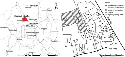
Our main data sources consist of daily GPS trajectories and activity diaries of urban residents living or working in the Shangdi-Qinghe area (Jiedao) of Beijing. As shown in Figure 1, the study area is located adjacent to the fifth ring road of Beijing in the north, about 16 km away from the city centre. Using a stratified random sampling approach, 709 respondents living or working in 23 neighbourhoods located in the study area were selected to participate in a seven-day survey from October to December in 2012 via eight waves (Ta et al. 2016). GPS tracking devices with a positional accuracy of about 15 m were used to record participants’ movement every 30 s for seven consecutive days. An interactive survey website consisting of two main components was developed: an activity diary component to collect detailed information on participants’ daily activities, and a questionnaire to collect socio-demographic and economic characteristics of participants.

Figure 1. The study area and key road networks in Beijing.

In this study, we work with complete daily trajectories, which is defined by using the criterion that the time gaps between any two sequential location records are all less than or equal to 10 min unless a participant is at home (information available from the diary data). Missing locations in a time period less than 10 min are assumed to be equally spaced between the start and end points of that period for simplicity. Based on a spatial threshold of 50 m and a temporal threshold of 10 min (time to conduct a meaningful activity), each participant’s daily movement trajectory was characterised as a sequence of consecutive stop and movement episodes, similar to the concept of syntactic trajectories in Grinberger and Shoval (2015). These trajectory episodes were then displayed on the website when a participant was filling in the activity diary at the end of each day to reduce recall bias (Kahneman et al. 2004). Both trajectory and activity diary data were passed on to a server and stored. As a quality control measure, we checked the completeness of the filled activity diary of each participant on the following day, and if an activity diary was incomplete, a text message would be sent to notify the participant of the issue. The stop episodes of trajectories were then matched with the reported activities and annotated with the attributes of matched activities and the socio-demographics of the corresponding participant. A match is achieved if the discrepancies in the start and end times between a stop episode and a reported activity period are both less than five minutes. In some cases when more than one activities are conducted in the same place (eg most often at home), a stop episode is further divided into a few episodes based on reported activity periods and annotated accordingly. Only matched activity episodes with complete information on key socio-demographic variables are included in the analysis. We further exclude respondents who are full-time students or unemployed as their daily activity arrangement could differ substantively from that of other groups of people (Shen et al. 2013). The final data includes 19,358 activities conducted by 494 participants in two to seven consecutive days (with a mode of five days). About 36% of the participants are dual earners of a family.

Our dependent variable is activity satisfaction, which is measured on a five-point Likert scale from being very dissatisfied (1) to being very satisfied (5). The mean activity satisfaction level is 3.77 with a standard deviation of 1.09 in our data (Table 1). The independent variables are broadly divided into several categories: situational activity characteristics, geographical context or activity space attributes, and individual-level socio-demographics. Although the impacts on general life satisfaction of individual socio-demographics have been extensively discussed (eg Diener et al. 1999, Kahneman et al. 2004, Ma et al. 2017), few studies have examined the potential link between activity satisfaction and characteristics of real-time geographical contexts where activities take place (Schwanen and Wang 2014).

Table 1. Variable description and summary statistics.

Variable names	Description	Mean or proportions
Dependent variable
Satisfaction	Activity satisfaction scores	3.77 (1.09)
Activity situational characteristics
Activity type
Maintenance	Maintenance activity	62.8%
Working	Working or subsistence activity	5.15%
Social and leisure	Social and leisure activities	17.5%
Others	Other activities	14.6%
Duration	Log of the lasting time of current activity (minutes)	148.1 (153.2)
Companion	An activity conducted with companions	53.3%
Travel time	Log of travel time from the preceding activity to the current activity (minutes)	43.9 (42.2)
Travel mode	Travel mode choices
Walking or cycling	Travel by walking or cycling	29.1%
Car	Travel by private car or taxi	29.7%
Public transport	Travel by bus or subway	31.3%
Other modes	Other travel modes used as baseline category	9.9%
Activity space characteristics
Density	Total floor areas in each land parcel
High	High land-use density	21.8%
Medium	Baseline category
Low	Low land-use density	34.3%
Land-use mix	The extent of land-use mix in each land parcel
High	High land-use mix	21.8%
Medium	Baseline category
Low	Low land-use mix	34.4%
Urban function	Dominating urban function of each land parcel
Green space	Green space function	9.0%
Residential	Residential function	29.4%
Commercial	Commercial function	4.8%
Other functions	Other urban functions used as baseline category
Individual-scale socio-demographic variables
Age	Age of the participant	33.6(8.22)
Monthly income (RMB^a)
	< 2,000	10.9%
	2,000–3,999	42.9%
	4,000–5,999	24.3%
	6,000–9,999	15.8%
	10,000 +	6.1%
Migrants	Without local household registration	32.6%
Child presence	Household with child or children under six years old	12.3%

^aRMB = renminbi, official Chinese currency.

To address this gap in the subjective well-being literature, the focus of our empirical investigation is on extending understandings of how situational urban environment, measured by fine spatial resolution urban form characteristics, affects activity satisfaction. More specifically, urban form was measured in three dimensions: land-use mix, density, and dominant function (Cervero and Kockelman 1997). These land-use characteristics were measured at the land parcel scale (an average size of about 0.03), which is the finest resolution land-use data publicly available in Beijing. Geographical extents of land parcels were delineated based on road networks by Beijing Institute of City Planning. Land-use mix and function are extracted based on points of interest (POI) data. In short, the function of a land parcel is inferred based on the dominant POI category in that parcel while land-use mix represents the diversity of POI categories, calculated by an entropy measure. Density is measured by the total floor areas in each land parcel. We refer to Liu and Long (2016) for a detailed description of the development of land-use characteristic variables. A standard GIS overlay operation was applied to the annotated trajectory episodes data and the spatial polygon land-use data to extract real-time urban environment characteristics of residents’ daily activities. Based on the upper and lower quantiles of land-use density and mix variables, a set of binary variables were generated to represent high, medium and low levels of density and mix. This is useful to explore potential non-linear land-use density and mix impacts on activity satisfaction, and to alleviate potential correlations between the two variables if treated as continuous. Our activity-scale measurement of urban environment takes into account participants’ daily mobility and thus tackling the uncertain geographic context problem (Kwan 2012) in the estimates of geographical contextual effects on subjective well-being.

The second set of independent variables is about activity situational characteristics such as type, duration and companionship. Respondents’ daily activities were originally coded into 19 specific categories in the web diary. To achieve a concise model specification, daily activities are divided into four broad categories: working or subsistence, maintenance, social and leisure, and others (eg Krizek 2003), as shown in Table 1. For instance, maintenance activities include sleeping, preparing food, eating, grocery shopping, and family obligation activities such as child care and shopping; social and leisure activities include socialising, social networking, exercising, while others include posting, banking, hospital visits and so on. Activity duration is the time that an activity lasts, which is treated as a continuous variable and differs greatly between activities (Table 1). Activity companionship is defined as a binary variable – whether an activity is conducted alone or with companions. To explore potential travel impacts on activity satisfaction, travel time from a preceding activity to the current activity and mode choices for the journey are included in the model.

The final set of independent variables are key individual socio-demographics. The linear and quadratic terms of age are included in the model to capture possible non-linear age impacts on activity satisfaction. Income was added to the model via a series of dummy variables (Table 1). Migrants (residents without Beijing hukou status) have been shown to be associated with lower global life satisfaction than local residents of Beijing (Dong et al. 2016, Ma et al. 2017). It is interesting to test whether migrants also tend to report lower satisfaction with daily activities. Family structure, represented by the variable child presence, was also incorporated in our model following previous studies (eg Ma et al. 2018). Descriptive statistics of each variable included in our analysis are provided in Table 1. The dependent variable was transformed to a standard Normal distribution while the independent variables including activity duration and travel time were log-transformed.

4. Model estimation results

As discussed above, the time threshold (or bandwidth) parameter is required when forming the temporal weights matrix or the spatially adjusted weights matrix (a space-time weights matrix for simplicity). Usually it was specified a priori or, in few cases, estimated along with other model parameters. Appealing as it sounds to calibrate from data, issues exist including additional computational cost and, more critically, great difficulties in distinguishing the estimation of and the temporal autoregressive parameter (eg Banerjee et al. 2014). The study adopts an alternative approach: selecting the value of that yields the best model fit from a finite set of possible values. Deviance information criterion (DIC, Spiegelhalter et al. 2002), the common model fit index in Bayesian inference that penalises model complexity, was used for model comparison and selection of . Smaller values of DIC indicate better model fits.

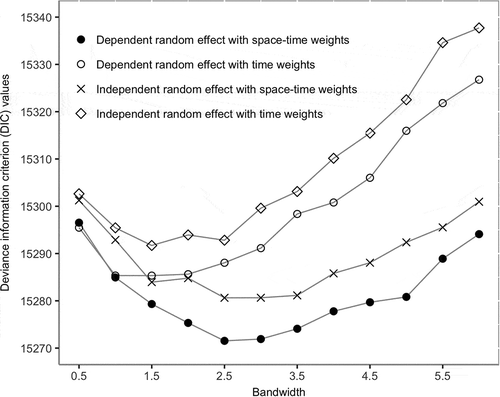
Twelve discrete values of over a range of were selected. Four models, treating individual random effects either as independent or dependent and with a time weights matrix or a space-time weights matrix , were estimated using the above MCMC samplers for each value of . Statistical inferences were based on two MCMC chains, each of which consisted of 10,000 iterations with a burn-in period of 5,000. Convergence of samplers was checked by visual inspection of trace plots of parameters and the Brooks-Gelman-Rubin scale reduction statistics (Brooks and Gelman 1998). The relationship between DIC and is illustrated in Figure 2. A clear result is the superior model fit offered by the model treating individual random effects as dependent (ie family interaction or correlation effects considered) and with a space-time weights matrix. For this preferred model specification, the optimal is 2.5 h. It is also noticeable that optimal values of are slightly different between model specifications. Moreover, it appears that models with a space-time weights matrix perform better than do models with a pure time weights matrix. This highlights the importance of taking into account both temporal and spatial distances between daily activities when exploring residents’ subjective experiences of activities.

Figure 2. Exploring the optimal time threshold parameter .

Regression coefficient estimates and the associated 95% credible intervals from the multi-level temporal autoregressive models with dependent individual random effects and a space-time weights matrix are reported in Table 2. As a comparison, estimation results from a multi-level temporal autoregressive models with a time weights matrix are also reported. Before proceeding to interpreting covariate effects on activity satisfaction, we discuss the estimates on structural model parameters. First, positive sequential or temporal correlations between activity satisfactions were found, indicated by the statistical significance of the temporal autoregressive parameter in both models. Putting the magnitude of temporal autocorrelation in perspective, for two activities separated by one hour, about 10.4% () of the satisfaction level of an activity would be carried over to the following activity, on average. Second, family correlation effects on activity satisfaction were identified, as indicated by the statistical significance of the autoregressive parameter at the 95% credible interval. A plausible explanation of the within-family correlations of daily activity satisfactions is the interacting decision process between family members in terms of daily activity arrangement. Third, is related to the magnitude of unobservable individual heterogeneity effect on activity satisfaction. In a standard multi-level model, the importance of individual heterogeneity effects can be quantified by the variance partitioning coefficient (, Goldstein 2011). This is not valid any more in our models with sequential correlations and dependent individual random effects, a similar issue found in the multi-level spatial econometric models (Dong and Harris 2015, Dong et al. 2015, Ma et al. 2017). To approximate the variance partitioning coefficient, we calculated marginal variances of the posterior residuals at the activity and individual scales. This yields an estimate on the variance partitioning coefficient of 0.44, indicating that about 44% of unexplained variances of activity satisfaction is due to unobservable individual heterogeneity effects. Overall, estimates on model structure parameters demonstrate complex dependencies in residents’ daily activity satisfaction, arising from both sequential correlations and individual heterogeneity effects.

Table 2. Model estimation results.

	Model with space-time weights			Model with time weights
Variables	Estimates			Estimates
	Median	2.5%	97.5%	Median	2.5%	97.5%
Activity situational characteristics
Maintenance	0.128*	0.095	0.161	0.129*	0.096	0.164
Social and leisure	0.151*	0.118	0.184	0.152*	0.119	0.187
Others	0.151*	0.111	0.19	0.152*	0.113	0.192
Duration	0.022	−0.016	0.058	0.023	−0.014	0.06
Duration squared	−0.056*	−0.098	−0.018	−0.058*	−0.097	−0.019
Companion	0.057*	0.04	0.075	0.057*	0.039	0.074
Travel time	−0.005*	−0.01	−0.001	−0.005*	−0.01	−0.001
Travel mode
Walking or cycling	0.02	−0.015	0.054	0.021	−0.014	0.054
Car	0.006	−0.033	0.045	0.006	−0.034	0.045
Public transport	0.032	−0.009	0.074	0.032	−0.009	0.073
Activity space characteristics
Land-use density
High	−0.021	−0.062	0.02	−0.021	−0.06	0.019
Low	0.005	−0.033	0.043	0.005	−0.032	0.043
Land-use mix
High	0.029	−0.013	0.071	0.03	−0.012	0.071
Low	−0.038*	−0.07	−0.005	−0.038*	−0.071	−0.005
Urban function
Green space	0.141*	0.083	0.198	0.142*	0.085	0.197
Residential	0.075*	0.036	0.115	0.075*	0.035	0.115
Commercial	−0.04	−0.105	0.024	−0.041	−0.104	0.027
Individual-scale socio-demographic variable
Age	−0.13*	−0.214	−0.032	−0.132*	−0.218	−0.039
Age squared	−0.082	−0.26	0.103	−0.071	−0.244	0.112
Monthly income (RMB)
< 2,000	−0.049	−0.157	0.067	−0.047	−0.174	0.064
2,000–3,999	0.022	−0.051	0.109	0.029	−0.061	0.111
6,000–9,999	0.005	−0.088	0.105	0.01	−0.099	0.121
10,000 +	0.033	−0.125	0.189	0.028	−0.132	0.192
Migrants	−0.121*	−0.198	−0.04	−0.12*	−0.194	−0.037
Child presence	−0.036	−0.142	0.057	−0.041	−0.157	0.067
	0.256*	0.237	0.276	0.253*	0.233	0.273
	0.385*	0.29	0.475	0.382*	0.286	0.47
	0.175	0.171	0.179	0.175	0.171	0.179
	0.119	0.103	0.138	0.121	0.104	0.14
DIC	15,250			15,265
N	19,358			19,358

Note: The symbol * indicates statistical significance at the 95% credible interval. .

Turning to the estimates on regression coefficients, we note that they represent the direct effects of independent variables on activity satisfaction. If a scalar summary of the total marginal effect of a variable was desired, one could calculate the average of row-sums of the matrix by plugging in respective parameter estimates. Table 2 shows that most situational activity characteristics and geographical contextual variables are statistically significantly associated with activity satisfaction. In terms of activity type, working is the least enjoyable activity comparing to other three activity types, ceteris paribus, which corroborates previous findings (Kahneman et al. 2004). Activity duration appears to be associated with satisfaction in a non-linear way as the coefficient of the quadratic duration term is statistically significant at the 5% significance level. Activity companionship makes a difference on satisfaction – activities conducted with companions tend to be more enjoyable than those conducted alone, holding other variables constant.

In terms of geographical contextual or activity space characteristics, land-use mix and urban function are statistically significantly associated with activity satisfaction. More specifically, conducting daily activities in places with low land-use mix tends to lower activity satisfaction, ceteris paribus. The difference in experiences of activities conducted in places with high or medium levels of land-use mix is, however, insignificant controlling for other variables. Urban functions of places where residents arrange activities also matter. Activities taking place in green space or residential areas are associated with higher levels of satisfaction comparing to those conducted in places with other urban functions, everything else being equal. Overall, these results suggest that characteristics of geographical contexts where activities take place are associated with residents’ subjective well-being of activities. This is in contrast with the findings in Schwanen and Wang (2014) that show no statistically significant relationships between activity space characteristics and satisfaction. A plausible explanation is that the relatively coarse-scale measurement of activity space attributes in Schwanen and Wang (2014) might not be able to characterise sites of activities accurately. In addition, the temporal autocorrelation in subjective well-being and individual heterogeneity effects are not properly captured in their model. Longer time spent on travel to conduct an activity is associated with lower activity satisfaction, holding other variables constant. However, travel mode choices do not appear to be correlated with activity satisfaction. Implications on urban planning would involve the promotion of mixed land uses to reduce travelling efforts in residents’ daily lives.

With respect to individual-scale variables, the linear term of age is statistically associated with activity satisfaction while the quadratic term is not. This, to some extent, departs from previous findings that age tends to be correlated with global life satisfaction non-linearly (eg Diener et al. 1999, Ma et al. 2017). The association between income and activity satisfaction was not statistically significant after controlling for the activity-level covariate effects on satisfaction. The lack of associations between the two key individual socio-demographic variables and daily activity satisfaction corroborates the argument that momentary satisfaction or affection relies more on situational circumstances and individual biological characteristics (part of the unobservable individual-scale effects) than life circumstance variables (Kahneman and Deaton 2010). Migrants, residents living in the city but without Beijing household registration (hukou), tend to report lower daily activity satisfaction than local residents. This might reflect the relatively limited space-time accessibility to quality opportunities for migrants due to them being subject to institutional constraints on access to affordable housing and social welfare systems such as education (eg Kwan 1999, Ma et al. 2017).

5. Conclusions

GPS trajectory or movement data have been increasingly explored to understand human mobility at fine spatio-temporal granularity. Integrating trajectory data with external data sources such as urban built environment and activity diaries to form semantic trajectories has been demonstrated to be of great value to promote knowledge on human activity and environment interactions (Grinberger and Shoval 2015, Siła-Nowicka et al. 2016). Nonetheless, dealing with the issues of time and scale for (semantic) GPS trajectory or movement data in a unified statistical model poses great challenges. This paper has proposed a novel multi-level temporal autoregressive model that deals with the two issues. In the model, time was conceptualised as continuous, allowing for a simple and intuitive way (ie a temporal weights matrix) to model sequential or temporal correlations between trajectory segments (daily activities in this study). Space is also introduced into the model, adjusting the temporal weights matrix on the basis of spatial distances between locations of activities. The scale issue is tackled by a simultaneous analysis of GPS trajectory data at different scales via a multi-level modelling approach.

The developed methodology is demonstrated by an empirical examination of residents’ daily activity satisfaction in Beijing, with a particular focus on how geographical contexts affect experiences of daily activities. Daily GPS trajectories of residents are annotated by using reported diary data, enabling rich characteristics to be extracted for trajectory episodes (activities in the study) and insights into relationships between activity satisfaction and situational urban environment at fine spatial resolution to be generated. A few key findings and the associated implications are worth highlighting. First, significant temporal or sequential correlations in daily activity satisfaction are found in models with a time or space-time weights matrix. It implies that treating activities or trajectory segments as independent in statistical models will be inappropriate. Individual heterogeneity effects account for a relatively large proportion of the variability in residents’ daily activity satisfaction, signifying the importance of individual heterogeneity in subjective well-being studies. Second, geographical contextual characteristics of sites where activities take place make a difference in experiences of activities – activities conducted in places with the higher land-use mix, lower density, and in green space tend to be associated with higher satisfaction levels. This, however, does not indicates that causal geographical contextual effects on activity satisfaction can be drawn due to the possible selection effect, ie people might intentionally choose sites with desirable characteristics for certain activities to pursue high levels of satisfaction. A pursuit of causal geographical contextual effect identification would require a simultaneous modelling of residents’ activity site choices and activity satisfaction (eg Steele 2008, Goldstein 2011), which is left for future research. Third, activity situational characteristics including types, duration and companionship are statistically significantly associated with satisfaction levels. Lastly, most of individual life circumstance variables are not significant correlates of daily activity satisfaction, with the exception of the migrant status.

Despite illustrated by examining residents’ activity satisfaction, the developed multi-level temporal autoregressive model is suitable to explore other characteristics of activities or trajectory segments. It also supplements the spatio-temporal statistics or econometrics literature (eg Elhorst 2014) by offering a useful tool to deal with data with irregular time intervals. Nevertheless, there are some limitations associated with the methodology. The first concerns the assumption that the temporal autoregressive parameter () is equal among individuals. This equal constraint is made for practical computational concerns, but it might be violated as it is possible that the strength of sequential correlations in daily activity satisfaction varies between individuals with distinct characteristics such as personalities. The second limitation regards the treatment of activity satisfaction as a continuous outcome variable. Activity satisfaction is, however, measured on a Likert scale, thus being an ordinal variable in nature (eg Dong et al. 2018). Ideally, it would be modelled as an ordinal response variable. These two extensions to the developed methodology are our next step of research. Thirdly, socio-demographic characteristics of activity space were not directly captured in our empirical satisfaction models due to the lack of data at fine-resolution spatial scale in the study area. However, as suggested in the spatial econometrics literature (LeSage and Pace 2009), the inclusion of a lagged dependent variable in our equation might capture the effect of these variables. Lastly, the formalisation of spatio-temporal relationships is based on distances between activities, but it would be extended to also consider movement speed in our future development such that the potential effect of travel congestion can be captured.

Acknowledgments

The authors are much grateful for the comments of the reviewers and the editor, which have greatly improved the content of the article. We also thanks Dr Xingjian Liu and Dr Ying Long for their great efforts of making the fine-resolution land use data in Beijing publicly available.

Disclosure statement

No potential conflict of interest was reported by the authors.

Additional information

Funding

This work was supported by the National Natural Science Foundation of China under Grants No.41601148 and No.41529101; Economic and Social Research Council [ES/P009301/1].

Notes on contributors

Guanpeng Dong

Guanpeng Dong is a lecturer in Geographic Data Science at the Department of Geography and Planning, University of Liverpool. His core research interests include spatial/spatiotemporal statistics and multi-level modeling methodological development and the application in urban studies. E-mail: [email protected]. 

Jing Ma

Jing Ma is an associate professor of Human Geography in Faculty of Geographical Science, Beijing Normal University. Her main research interests include activity-travel behaviour, subjective well-being, environmental justice and health. E-mail: [email protected] or [email protected].

Mei-Po Kwan

Mei-Po Kwan is a professor at the Department of Geography and Geographic Information Science, University of Illinois at Urbana-Champaign. Her research addresses health, transport, environmental, and social issues through the application of innovative geographic information system (GIS) methods.

Yiming Wang

Yiming Wang is a senior lecturer at the School for Policy Studies, University of Bristol. His research involves analysing economic and social policies through the application of both quantitative and qualitative methods.

Yanwei Chai

Yanwei Chai is a professor at the College of Urban and Environmental Sciences, Peking University. His research interests include behavioural geography and time geography.

References

- Anselin, L., 1988. Spatial econometrics: methods and models. Dorddrecht: Kluwer Academic Publishers.
- Asar, Ö., et al. 2016. Short-term and long-term effects of acute kidney injury in chronic kidney disease patients: A longitudinal analysis. Biometrical Journal, 58 (6), 1552–1566. doi:10.1002/bimj.201500156
- Banerjee, S., Carlin, B.P., and Gelfand, A.E., 2014. Hierarchical modeling and analysis for spatial data. Boca Raton: CRC Press.
- Bates, D. and Maechler, M., 2017. Matrix: sparse and dense matrix classes and methods. R package version 1.2-12. Available from: http://cran. r-project. org/package=Matrix
- Brooks, S.P. and Gelman, A., 1998. General methods for monitoring convergence of iterative simulations. Journal of Computational and Graphical Statistics, 7 (4), 434–455.
- Browne, W. and Goldstein, H., 2010. Mcmc sampling for a multilevel model with nonindependent residuals within and between cluster units. Journal of Educational and Behavioral Statistics, 35 (4), 453–473. doi:10.3102/1076998609359788
- Cervero, R. and Kockelman, K., 1997. Travel demand and the 3ds: density, diversity, and design. Transportation Research Part D: Transport and Environment, 2 (3), 199–219. doi:10.1016/S1361-9209(97)00009-6
- Demšar, U. and Virrantaus, K., 2010. Space–time density of trajectories: exploring spatio-temporal patterns in movement data. International Journal of Geographical Information Science, 24 (10), 1527–1542. doi:10.1080/13658816.2010.511223
- Diener, E., et al., 1999. Subjective well-being: three decades of progress. Psychological Bulletin, 125 (2), 276. doi:10.1037/0033-2909.125.2.276
- Diggle, P., 2002. Analysis of longitudinal data. Oxford: Oxford University Press.
- Diggle, P.J., Sousa, I., and Asar, Ö., 2014. Real-time monitoring of progression towards renal failure in primary care patients. Biostatistics, 16 (3), 522–536. doi:10.1093/biostatistics/kxu053
- Dodge, S., Laube, P., and Weibel, R., 2012. Movement similarity assessment using symbolic representation of trajectories. International Journal of Geographical Information Science, 26 (9), 1563–1588. doi:10.1080/13658816.2011.630003
- Dong, G. and Harris, R., 2015. Spatial autoregressive models for geographically hierarchical data structures. Geographical Analysis, 47 (2), 173–191. doi:10.1111/gean.2015.47.issue-2
- Dong, G., et al., 2015. Multilevel modelling with spatial interaction effects with application to an emerging land market in beijing, china. PloS One, 10 (6), e0130761. doi:10.1371/journal.pone.0130761
- Dong, G., et al., 2016. Spatial random slope multilevel modeling using multivariate conditional autoregressive models: A case study of subjective travel satisfaction in beijing. Annals of the American Association of Geographers, 106 (1), 19–35. doi:10.1080/00045608.2015.1094388
- Dong, G., Nakaya, T., and Brunsdon, C., 2018. Geographically weighted regression models for ordinal categorical response variables: an application to geo-referenced life satisfaction data. Computers, Environment and Urban Systems, 70, 35–42. doi:10.1016/j.compenvurbsys.2018.01.012
- Dungan, J.L., et al., 2002. A balanced view of scale in spatial statistical analysis. Ecography, 25 (5), 626–640. doi:10.1034/j.1600-0587.2002.250510.x
- Elhorst, J.P., 2010. Applied spatial econometrics: raising the bar. Spatial Economic Analysis, 5 (1), 9–28. doi:10.1080/17421770903541772
- Elhorst, J.P., 2014. Spatial econometrics: from cross-sectional data to spatial panels. Heidelberg: Springer.
- Gelman, A., et al., 2014. Bayesian data analysis. FL: CRC press Boca Raton.
- Goldstein, H., 2011. Multilevel statistical models. Chichester: John Wiley & Sons.
- Grinberger, A.Y. and Shoval, N., 2015. A temporal-contextual analysis of urban dynamics using location-based data. International Journal of Geographical Information Science, 29 (11), 1969–1987. doi:10.1080/13658816.2015.1049951
- Haining, R.P., 2003. Spatial data analysis: theory and practice. Cambridge: Cambridge University Press.
- Harris, R., Dong, G., and Zhang, W., 2013. Using contextualized geographically weighted regression to model the spatial heterogeneity of land prices in beijing, china. Transactions in GIS, 17 (6), 901–919. doi:10.1111/tgis.2013.17.issue-6
- Hsiao, C., 2014. Analysis of panel data. Cambridge: Cambridge university press.
- Huang, B., Wu, B., and Barry, M., 2010. Geographically and temporally weighted regression for modeling spatio-temporal variation in house prices. International Journal of Geographical Information Science, 24 (3), 383–401. doi:10.1080/13658810802672469
- Hughes, R.A., et al., 2017. Estimation of the linear mixed integrated ornstein–uhlenbeck model. Journal of Statistical Computation and Simulation, 87 (8), 1541–1558. doi:10.1080/00949655.2016.1277425
- Kahneman, D., et al. 2004. A survey method for characterizing daily life experience: the day reconstruction method. Science, 306 (5702), 1776–1780. doi:10.1126/science.306.5698.956a
- Kahneman, D. and Deaton, A., 2010. High income improves evaluation of life but not emotional well-being. Proceedings of the National Academy of Sciences, 107 (38), 16489–16493. doi:10.1073/pnas.1011492107
- Krizek, K.J., 2003. Neighborhood services, trip purpose, and tour-based travel. Transportation, 30 (4), 387–410. doi:10.1023/A:1024768007730
- Kwan, M.P., 1999. Gender and individual access to urban opportunities: a study using space–time measures. The Professional Geographer, 51 (2), 210–227. doi:10.1111/0033-0124.00158
- Kwan, M.P., 2012. The uncertain geographic context problem. Annals of the American Association of Geographers, 102 (5), 958–968. doi:10.1080/00045608.2012.687349
- Kwan, M.P. and Neutens, T., 2014. Space-time research in giscience. International Journal of Geographical Information Science, 28 (5), 851–854. doi:10.1080/13658816.2014.889300
- Kwan, M.P., Xiao, N., and Ding, G., 2014. Assessing activity pattern similarity with multidimensional sequence alignment based on a multiobjective optimization evolutionary algorithm. Geographical Analysis, 46 (3), 297–320. doi:10.1111/gean.12040
- Lee, L.F. and Yu, J., 2010. Some recent developments in spatial panel data models. Regional Science and Urban Economics, 40 (5), 255–271. doi:10.1016/j.regsciurbeco.2009.09.002
- LeSage, J. and Pace, R.K., 2009. Introduction to spatial econometrics. Boca Raton: CRC Press.
- Liu, X. and Long, Y., 2016. Automated identification and characterization of parcels with openstreetmap and points of interest. Environment and Planning B: Planning and Design, 43 (2), 341–360. doi:10.1177/0265813515604767
- Long, J.A. and Nelson, T.A., 2013. A review of quantitative methods for movement data. International Journal of Geographical Information Science, 27 (2), 292–318. doi:10.1080/13658816.2012.682578
- Ma, J., et al., 2018. Does satisfactory neighbourhood environment lead to a satisfying life? an investigation of the association between neighbourhood environment and life satisfaction in beijing. Cities, 74, 229–239. doi:10.1016/j.cities.2017.12.008
- Ma, J., et al., 2017. Inequality in beijing: A spatial multilevel analysis of perceived environmental hazard and self-rated health. Annals of the American Association of Geographers, 107 (1), 109–129. doi:10.1080/24694452.2016.1224636
- Parent, C., et al., 2013. Semantic trajectories modeling and analysis. ACM Computing Surveys (CSUR), 45 (4), 1–32. doi:10.1145/2501654
- Parent, O. and LeSage, J.P., 2012. Spatial dynamic panel data models with random effects. Regional Science and Urban Economics, 42 (4), 727–738. doi:10.1016/j.regsciurbeco.2012.04.008
- Purves, R.S., et al., 2014. Moving beyond the point: an agenda for research in movement analysis with real data. Computers, Environment and Urban Systems, 47, 1–4. doi:10.1016/j.compenvurbsys.2014.06.003
- Raudenbush, S.W. and Bryk, A.S., 2002. Hierarchical linear models: applications and data analysis methods. Thousand Oaks, CA: Sage.
- Schwanen, T. and Wang, D., 2014. Well-being, context, and everyday activities in space and time. Annals of the Association of American Geographers, 104 (4), 833–851. doi:10.1080/00045608.2014.912549
- Searle, S.R. and Khuri, A.I., 2017. Matrix algebra useful for statistics. New Jersey: John Wiley & Sons.
- Shen, Y., Kwan, M.P., and Chai, Y., 2013. Investigating commuting flexibility with gps data and 3d geovisualization: a case study of beijing, china. Journal of Transport Geography, 32, 1–11. doi:10.1016/j.jtrangeo.2013.07.007
- Siła-Nowicka, K., et al., 2016. Analysis of human mobility patterns from gps trajectories and contextual information. International Journal of Geographical Information Science, 30 (5), 881–906. doi:10.1080/13658816.2015.1100731
- Spaccapietra, S., et al., 2008. A conceptual view on trajectories. Data & Knowledge Engineering, 65 (1), 126–146. doi:10.1016/j.datak.2007.10.008
- Spiegelhalter, D.J., et al., 2002. Bayesian measures of model complexity and fit. Journal of the Royal Statistical Society: Series B (Statistical Methodology), 64 (4), 583–639. doi:10.1111/rssb.2002.64.issue-4
- Steele, F., 2008. Multilevel models for longitudinal data. Journal of the Royal Statistical Society: Series A (Statistics in Society), 171 (1), 5–19.
- Ta, N., Kwan, M.P., and Chai, Y., 2016. Urban form, car ownership and activity space in inner suburbs: A comparison between beijing (china) and chicago (united states). Urban Studies, 53 (9), 1784–1802. doi:10.1177/0042098015581123
- Taylor, J.M., Cumberland, W., and Sy, J., 1994. A stochastic model for analysis of longitudinal aids data. Journal of the American Statistical Association, 89 (427), 727–736. doi:10.1080/01621459.1994.10476806
- Yan, Z., et al., 2013. Semantic trajectories: mobility data computation and annotation. ACM Transactions on Intelligent Systems and Technology, 4 (3), 1–34. doi:10.1145/2483669
- Yang, C. and Gidófalvi, G., 2017. Mining and visual exploration of closed contiguous sequential patterns in trajectories. International Journal of Geographical Information Science.doi:10.1080/13658816.2017.1393542