Distinguishing extensive and intensive properties for meaningful geocomputation and mapping

ABSTRACT

A most fundamental and far-reaching trait of geographic information is the distinction between extensive and intensive properties. In common understanding, originating in Physics and Chemistry, extensive properties increase with the size of their supporting objects, while intensive properties are independent of this size. It has long been recognized that the decision whether analytical and cartographic measures can be meaningfully applied depends on whether an attribute is considered intensive or extensive. For example, the choice of a map type as well as the application of basic geocomputational operations, such as spatial intersections, aggregations or algebraic operations such as sums and weighted averages, strongly depend on this semantic distinction. So far, however, the distinction can only be drawn in the head of an analyst. We still lack practical ways of automation for composing GIS workflows and to scale up mapping and geocomputation over many data sources, e.g. in statistical portals. In this article, we test a machine-learning model that is capable of labeling extensive/intensive region attributes with high accuracy based on simple characteristics extractable from geodata files. Furthermore, we propose an ontology pattern that captures central applicability constraints for automating data conversion and mapping using Semantic Web technology.

KEYWORDS:

• Extensive and intensive properties
• geocomputation
• mapping
• automated semantic labeling of geodata
• meaningful analysis

1. Introduction

Map making and geocomputation are two essential crafts analysts need to master in order to extract knowledge from geographic data and to gain insights from data analysis using Geographic Information Systems (GIS). Yet, we know that the practice of map making as well as the analytical process are full of semantic intricacies that require a lot of training. Cartographic practice, for instance, entails a large amount of written and unwritten ‘rules’ about scales of measurement, data semantics and analytic intentions when selecting graphical symbols on a map (Müller et al. 1995). In a similar fashion, the application of GIS tools to construct geocomputational workflows is an art that goes largely beyond fitting data types to inputs and outputs (Hofer et al. 2017). In fact, meaningful analysis, i.e. the application of appropriate analytic methods to data sources of a specific origin for a given purpose (Stasch et al. 2014, Scheider and Tomko 2016), requires considerable background knowledge about semantic concepts.

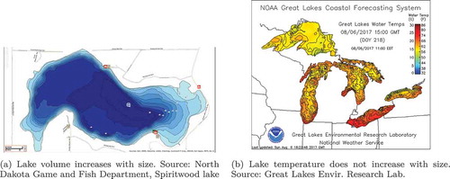
Consider the following example. Suppose we have one region attribute representing lake temperatures measured by environmental sensors, and another one denoting water volumes of these same lakes. Both have the same data type (polygon vector data). Suppose that for purposes of estimating hydroelectric energy potentials, we are interested in the water volume of all lakes as well as in the temperature of the water, in order to assess to what extent heating up by the power plant may lead to ecological damage downstream (Bobat 2015). For a skilled analyst, it is intuitively clear that total volume can be obtained by summing up lake volumes, whereas each measured temperature value needs to be weighted by the volume of the respective lake to arrive at a reliable estimate of the water’s average temperature. Furthermore, this analyst is likely to choose a choropleth map when visualizing lake temperature over space, but a bar chart or pie chart map for lake volume. The reason lies in the fact that intensive measures like temperature are independent on the size of their supporting object (in this case the area of the lake’s region, see Figure 1(b)), while extensive measures, such as lake volume, are additive (Figure 1(a)).

Figure 1. Examples of extensive and intensive properties. Image (a) by kind permission of North Dakota Game and Fish department. Image (b) by open attribution license (CC BY).

As this simple example illustrates, deciding about the meaningfulness of many cartographic and geo-analytic methods requires distinguishing between extensive and intensive measures. While this might look like a trivial problem for a human analyst, it is very difficult for a computer to decide without any human intervention, since nothing in a data type or a computational property reveals the matter. Yet, automation is required in order to scale up geocomputation and mapping over the extensive amount of data sets at our disposal. We need technology that makes tool and geodata diversity manageable by automatizing analytic tasks. The reasons that prevent us from exploiting these semantic distinctions are at least twofold (cf. Scheider et al. (2017)):

1. We lack methods for automatic labeling of data sets and attributes with extensiveness/intensiveness. Manual labeling is seldom done in practice and does not scale with the speed of data production (Alper et al. 2015).

2. We lack methods for systematically assessing the space of meaningful geocomputational/cartographic method applications to extensive/intensive properties. In essence, we lack a theory that would allow us to explore this space in a systematic manner once data are labeled.

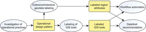
In this article, we address both challenges through investigating possible solutions from machine learning (ML) and geospatial semantics (Egenhofer 2002, Janowicz et al. 2013). For tackling the first challenge, we test several supervised ML classification algorithms on different kinds of (geo-)statistical features extracted from region statistics data which capture the relation between areas and their attributes (Section 3). Regarding the second challenge, we review textbook knowledge about the applicability of cartographic and geocomputational methods and encode it using an algebraic model expressed in terms of an ontology design pattern (Section 4). Together with the result of geodata labeling, this pattern can be used to select kinds of GIS tools adequate for intensive (IRA) and extensive region attributes (ERA), for workflow automation and data/tool recommendation on statistical portals (compare Figure 2). We explain each method, discuss its results and give an outlook in the corresponding sections. We start with reviewing the state of the art about extensive and intensive properties.

Figure 2. Approach taken in this article. We suggest an operational design pattern and test approaches for labeling statistical attributes and corresponding GIS tools. Workflow automation and data/tool recommendation are considered future work.

2. State of the art regarding intensive/extensive properties

In order to understand how the distinction between intensive and extensive properties affects mapping and analysis, we review previous work in this section. We discuss the role in Cartography and geocomputation, as well as previous efforts of theoretical systematization and computation.

2.1. The origins

The official definition of the two concepts is laid down in the Compendium of Chemical Terminology published by the International Union of Pure and Applied Chemistry (IUPAC) (Cohen 2007), as Chemistry is their field of origin. This compendium, also informally known as the ‘Goldbook’ after its original first author, gives the following definitions (McNaught and McNaught 1997):

• Intensive quantity: ‘Physical quantity whose magnitude is independent of the extent of the system’.

• Extensive quantity: ‘Physical quantity whose magnitude is additive for subsystems’

Redlich (1970) gives a similar definition:

Most of the properties which we measure quantitatively may be divided into two classes. If we consider two identical systems, let us say two kilogram weights of brass or two exactly similar balloons of hydrogen, the volume, or the internal energy, or the mass of the two is double that of each one. Properties of this type are called extensive. On the other hand, the temperature of the two identical objects is the same as that of either one, and this is also true of the pressure and the density. Properties of this type are called intensive.

The concept pair of spatial intensiveness and spatial extensiveness was introduced first by Tolman (1917). At that time, it was meant as a tool in Chemistry and Thermodynamics, two areas where these concepts are still frequently used today (Canagaratna 1992). However, the concepts have been established in the Geosciences as well. The earliest mention we could find was in Goodchild and Lam (1980), some six decades after Tolman. Goodchild and Lam however mention them only en passant. A proper introduction into the Geosciences was done by ‘spatial philosopher’ Gilles Deleuze, known for popularizing terms like smooth and striated, nomadic and sedentary, deterritorialization and reterritorialization (Deleuze 1994, Buchanan and Lambert 2005).

Still, extensiveness and intensiveness seem relatively underused concepts of science (Canagaratna 1992). Lobato and Thanheiser (1999) argue that the distinction between intensive and extensive qualities is crucial when teaching about rates, such as speed. In recent years, the concept pair has also found traction within the industry. Mijnarends et al. (2015) e.g. illustrated its use in estimating various flow rates and designing useful maps for the oil industry, as well as for designing comprehensive GIS to manage such work.

Not all quantities are either intensive or extensive. Some quantities behave so erratically that it is difficult if not impossible to classify them in this way. In addition, some quantities have a dimensionality that is too low for this purpose (Jaeger 2000). Point vector data for example are 0-dimensional and thus cannot be classified with regards to the behavior toward their extent. They may therefore not fall under this dichotomy (Jaeger 2000).

Finally it is worth mentioning the work of Gorenstein and Gadzicki who further specify the intensive–extensive concept pair into strongly and weakly intensive properties. Strongly intensive properties are those properties which do not depend on the extent whatsoever. Weakly intensive properties are semi-dependent on extent (Gorenstein and Gadzicki 2011). Following the IUPAC definition, weakly intensive properties are extensive properties. In this paper, we will stick to the IUPAC definition.

2.2. The role in cartographic best practice

In his seminal work, Bertin et al. (1967) proposed a systematic account of map types together with graphic variables, which unfortunately lacks any reference to extensiveness or intensiveness. Cartographers are nevertheless aware of the cartographic implications of these concepts, even though today’s standard books about methods of map visualization do not mention them explicitly.¹

In fact, a considerable part of the intuitive cartographic perception and interpretation rules depend on the intensive–extensive distinction. A prominent example is the appropriateness of applying choropleth maps, proportional symbol maps and isopleth maps. As elaborated by Lin et al. (2017), choropleth maps are only appropriate for displaying intensive data, because color is perceived as independent from (orthogonal to) size. Since choropleth maps consist of graduated color areas of polygons of varying sizes, large polygons would automatically stand out when extensive properties were to be mapped in this way. This would produce an incorrect impression of the phenomenon under study, with large areas seeming more important than they really are, not by virtue of the phenomenon, but due to their size. A practical example of this effect is given in Figure 3, where (a) causes a wrong impression about the distribution of population across the United States. In the case of the proportional symbol map (e.g. a map where the size of circles denotes the attribute value of a region), in contrast, we expect the size of the symbol to vary with the size of the enclosing area. Furthermore, attribute values are visually expressed by another kind of size (the size of the symbol). This makes this type of map appropriate for extensive properties.

Figure 3. Extensive data such as depicted in (a) distort the perception of the phenomenon due to the differing sizes of the area units. The intensive data depicted in (d), in this case population density, show the actual pattern shown in (c) much more accurately. Proportional symbols (b) do not have such a distorting effect and thus can be safely used with extensive data. Isopleth maps (e) should only be used with intensive values. Population data gathered from US Census Bureau (2017), night illumination data acquired from NASA’s Earth Observatory (Stevens 2016), Lambert equal area conic projection.

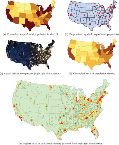
In comparison to choropleth and proportional symbol maps, isopleth maps exclusively represent intensive measures. These maps denote a continuous value field consisting of point-like measures which lack a spatial size and thus are bound to be considered intensive. Furthermore, cartographic regionalizations and cartographic aggregations are likewise affected by the intensive–extensive distinction (Kyriakidis 2017, Lin et al. 2017, She et al. 2017).

We conclude that extensive and intensive properties could be utilized as part of an automated map making program. For instance, a script could be written which displays intensive data using class interval selection rules as laid down by Evans (1977).

2.3. The role in geocomputation and spatial analysis

The distinction between intensive and extensive properties is also crucial in many commonly occurring analytic and geocomputational tasks in GIS. In the following, we quickly review a number of well-known practices involving different types of GIS operations and geodata formats, without claiming that these cases cover all methods that might be affected by the distinction.

First, consider aggregating attributes of two areas A and B. In order to aggregate A and B into a new area (see Figure 4(b)), we need to decide whether or not we should add the two values or take their average. This depends on whether the data are extensive or intensive. If A and B are values of an extensive variable, like total population measures, then a simple sum is required to aggregate the attributes into the merger of their regions. If A and B are values of an intensive variable, like the gross domestic product (GDP) per capita, then a weighted average needs to be used (Kyriakidis 2017, She et al. 2017).

Figure 4. Areal interpolation and spatial disaggregation.

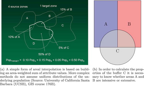
Second, consider the case of subdividing or modifying region layers, which involves a disaggregation. For example, suppose there is a layer with total population in administrative regions, and we are interested in estimating the population in a layer with overlapping regions, e.g. electoral districts. One of the simplest methods is based on assuming a homogeneous distribution of the underlying population and building an area-weighted sum of population attributes (Figure 4(a)). The population values in this case need to be extensive (given as total sum), not intensive. More sophisticated interpolation procedures rely on Kriging of the underlying population density surface (Krivoruchko et al. 2011). Note that the latter method requires intensive properties as input and internally deals with intensive–extensive data conversions. A similar problem concerns resampling of a raster layer into a new layer that overlaps with the raster cells.² Raster values of remote-sensing images, such as radiation intensity values, are intensive, not extensive. In practice, simple ad-hoc interpolation techniques are often used, e.g. assigning the intensive value of the nearest raster cell (Burrough 1986).

Another disaggregation occurs when intersecting buffer regions with a statistical region layer (e.g. about populations numbers) to estimate environmental interaction effects (e.g. the impact of a road on surrounding residents). If the attribute is extensive (e.g. population counts) and if we want to calculate the aggregated value of the intersection of A and B with buffer C (Figure 4(b)), the fraction of intersected area for both A and B would have to be calculated. If A and B represent two values of an intensive variable (e.g. population density), one may compute an area-weighted average of the attribute values of A and B.

In geoprocessing, such rules are sometimes referred to as split and merge rules or policies (Goodchild et al. 2007).³

2.4. Previous efforts of systematization and automation

A number of attempts have been made to systematize and exploit such practical insights in terms of theoretical and computational approaches.

In spatial statistical analysis, an issue closely related to the size and shape of regions is the Modifiable Area Unit Problem (MAUP) (Openshaw 1984b). It has been known for a long time that statistical moments and indicators (such as correlations) are significantly affected by the way how underlying phenomena (base units) are summarized into regions, both by aggregating to larger regions, as well as by reshaping regions in different ways. Textbooks often present MAUP with examples that assume extensiveness (Kemp 2007, p. 112). Studying the relevant literature (Openshaw 1984a, 1984b, Fotheringham and Wong 1991, Jelinski and Wu 1996), we could however not identify a discernible role that these concepts should play in defining or curing MAUP. In fact, it is implicitly assumed in these articles that statistics were computed based on intensive (‘normalized’) attributes (such as the correlation between population density and poverty rates), to make results independent from a region’s size. In these texts, MAUP is comprehended as a problem of reconstructing base unit statistics (e.g. estimating correlations on higher resolution levels, such as households). Yet, MAUP is also understood by scholars in a slightly different way, namely as the problem of reconstructing attributes for these base units themselves (Jones 2014, p. 211), compare the examples of disaggregation in Section 2.3. This latter problem has in fact a clear link to intensiveness and extensiveness (Flowerdew and Green 1993), which we will specify in Section 4. However, we think it is better captured by the term areal interpolation.

In contemporary Geographic Information Science (GIScience), the concept pair often contributes to a more general methodological approach to data analysis and geodata. Textbooks use it to explain the difference between choropleth and isopleth maps (Longley et al. 2005, p. 96). Goodchild et al. (2007) used intensiveness for introducing a fundamental building block of geographic information, the geo-atom. Lin et al. (2017) proposed to use the distinction in order to handle isopleth mapping. She et al. (2017) suggested a method for minimizing region heterogeneity based on distinguishing intensive and extensive properties, and in Kyriakidis (2017), the distinction forms part of a method for aggregation of geodata. In Scheider and Tomko (2016), we have proposed an ontology that captures applicability constraints of analytical methods based on distinguishing measures from regions which support attributes (cf. Section 4.1). However, none of these previous attempts have addressed how the distinction could be formally captured together with GIS methods and how it could be used in labeling data sets for automated geocomputation. We would like to stress that the distinction is not captured either by any scale type or level of measurement. Measurement levels (such as ratio, interval, ordinal) are defined as morphisms on a single domain (Suppes and Zinnes 1963), while extensiveness is a relation between two different domains, namely measures and sizes of supporting regions.⁴

In Cartography, it is commonly acknowledged that map making is an inherently human process difficult to automatize, because computers have trouble dealing with the perceptual properties of the symbology involved (Müller et al. 1995). Still, computers could enhance the process of map making more than they currently do, by accounting for some of the best practices in Cartography. This requires ordering these practices around semantic concepts, e.g. in terms of ontologies on the Semantic Web using linked data (Bizer et al. 2009). This was recently done for map scaling and generalization (Carral et al. 2013, Stern and Sester 2013) and for map mash ups (Tooamnian et al. 2013, Huang et al. 2018). However, to the best of our knowledge, the semantic distinction under study has never been subject of corresponding ontological or computational studies.

3. Classification of region attributes into intensive and extensive

How well can we automatize the labeling of region attributes in geodata sets? In this section, we compute a range of statistics over region attribute data and use them as features to classify data sets into either extensive or intensive, using various ML methods. Since these classes are considered mutually exclusive, this is a single-label supervised classification problem.⁵ The Python scripts for geodata set classification can be found on github.⁶

3.1. Challenges in statistically classifying region data sets

Given the simplicity of the definition of our target concepts, one may wonder whether it is difficult at all to determine whether a given attribute falls in either of these classes based on the statistical association between region size and attribute value. However, as we will show in Section 3.6, it turns out that the statistical association is rather weak and unfortunately not enough to learn these concepts. We suspect the reason for this lies in the fact that a layer consisting of predefined statistical or administrative regions is a very biased sample of all possible areal aggregations of an underlying phenomenon. It is very improbable that the size of these regions is uniformly distributed over different resolution levels and different locations, and thus the effect of increased attribute value with size, which would appear in an independent regional sample, may be canceled out by sampling small regions at locations with high phenomena concentrations and large regions at locations with low concentrations. This problem is in fact a variant of the ecological fallacy and MAUPs (Openshaw 1984b), and it has very similar consequences. In very extreme cases, it could even lead to the effect that the association between size and attribute value is negative. For this reason, it is not at all obvious whether this inference can be made, and if yes, based on which features of a region data set.

3.2. Training and test data sets

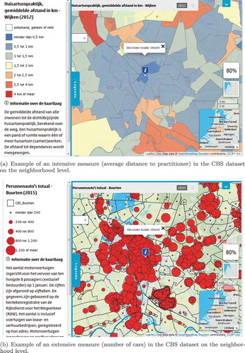
The used data sets originate from the ‘Kerncijfers Wijken en Buurten’ (KWB) provided by the Dutch statistics agency, the ‘Centraal Bureau voor de Statistiek’ (CBS).⁷ This data set was chosen because it provides a large number of statistical variables on different scale levels in a readily usable shapefile format. In total, these are 193 variables for 3 different regional aggregate levels inside the Netherlands, namely neighborhoods, boroughs and municipalities (CBS 2014). The variables include demographical, economic, social and topographic phenomena, such as a_pau: Personenauto’s totaal [aantal], denoting the total number of carryall vehicles in a region, and g_afs_hp: Afstand tot huisartsenpraktijk [km], denoting the distance to the nearest practitioner averaged for all households in a region (see Figure 5). Only two variables from this set were excluded from the analysis because they contained only missing values.

Figure 5. Test data from the portal ‘CBS in uw buurt’, accessible online under http://www.cbsinuwbuurt.nl/.

3.3. Explanatory features of region attributes

The core of our classification method lies in the appropriate selection of features of region attributes. For this study, statistical and spatial statistical measures (De Smith et al. 2007) were tested as predictors, based on the idea that various indicators of spatial and nonspatial association together might best be able to uncover a covert relation between attribute measures and regions. Note that our indicators all exploit some quality of a region, either its size or spatial configuration, together with its attribute value. In this subsection, indicators are discussed and a rationale is given for their inclusion in the study.

• Linear regression intercept: The intercept of the regression equation of a given KWB quantity plotted against the area of its support polygons. This feature is expected to be important in distinguishing intensive and extensive attributes since extensive measures are supposed to approximate an intercept of zero. A region extent of zero causes extensive measures to become zero.

• Linear regression slope: This feature of the regression equation of a given KWB quantity plotted against the area of its support polygons might also be of use. An ERA is expected to have a significant positive slope since its measure is expected to rise with the region extent.

• Pearson’s R: This feature captures the strength of the correlation between the region’s area and the KWB quantity based on their covariance.

• $R^2$: This feature captures the ratio of the explained versus the total covariance of a KWB quantity plotted against the region’s area. It cannot become negative in contrast to Pearson’s R, of which it is the square.

• Levene’s W: This feature captures homoscedasticity in the linear regression of the KWB quantity plotted against the area of its support polygons. If the input data have highly differing variances for small and large areas, this might indicate that it is not strictly a function of area and a linear model does not well capture the relation between them.

• Median of residuals: This is a feature which complements Levene’s W in assessing whether linear regression residuals might not be homoscedastic.

• Median of secondary residuals: This feature complements Levene’s W, where high values would indicate that the residuals of the linear regression might not be homoscedastic.

• Moran’s I: A feature capturing spatial autocorrelation in the region attribute data set. High values spatially surrounded by low values and vice versa result in a low score. Autocorrelation measures are used here because they indicate whether areas with similar sizes are spatially clustered with regions of similar values, and thus whether the areal sample is biased (compare Section 3.1). This is the case when e.g. small regions are grouped together and have similarly low attribute values.

• Z-value of I: Likelihood of the occurrence of Moran’s I autocorrelation in the input data.

• Getis–Ord G: A feature capturing the grouping of region attribute values into hot spots, where high values are surrounded by a smooth decrease into the neighborhood. High values surrounded by low values result in a high score.

• Z-value of G: Likelihood of the occurrence of the Getis–Ord G measure given the input data.

3.4. Data preprocessing

The training data set consisted of a list of features for each region attribute in the KWB source together with a class label indicating whether it was extensive or intensive. These data were prepared using a Python script.⁸

The KWB data set bundles various survey and census results in three shapefiles for each of the three regional aggregation levels. These were first split into 519 separate shapefiles each containing only 1 variable for 1 scale level. Subsequently, these shapefiles were checked for projection information, and unprojected data were projected using the ArcPy module in order to assure faithful area assessments. Once the layer in question was projected, the areal extent of the polygons within the layer was calculated. Region sizes were extracted with two ArcPy tools, Calculate Geometry⁹ and Project.¹⁰ Doing so allowed the creation of a small layer with just one attribute containing the KWB quantity and one variable containing the area of each polygon. The explanatory features used for the classification were then computed with ArcPy (Moran’s I and Getis–Ord G spatial autocorrelation measures) as well as the linear regression function of Scikit Learn. The ML classifier tools were all part of the Scikit Learn library (Pedregosa et al. 2011). With this groundwork done, attributes were z-normalized for all 519 different layers. The preparation script was profiled to determine the approximate runtime of each of the classifiers for these data. We used the line profiler developed by Robert Kern.¹¹

Finally, we manually labeled these layers by consulting CBS’s metadata. Filenames were collected and manually tagged as either intensive or extensive, depending on the textual description in the metadata and the data type of the KWB quantity.

3.5. ML classifier selection, training and testing

Ten different supervised ML classifiers (Friedman et al. 2001) were tested on the data. The logistic regression classifier was excluded from the study because initial tests suggested that it performed significantly worse. While the internal functions and the expected behavior of some classifiers like decision trees are easily understood, others like the Multilayer Perceptron neural net are more opaque. In order to better interpret the results, we give a short summary of each in the following paragraph.

• The Decision Tree classifier models the input data based on a tree, where each node is a binary decision rule about some feature. A maximum tree depth of five decision rules was used to prevent overfitting. Decision rules can capture nonlinear relationships; however, they are unable to model smooth class borders.

• The Adaptive Boosting (AdaBoost) classifier combines the output of multiple decision trees based on weak predictors to arrive at a weighted sum that forms the final boosted classifier. This classifier can be expected to work better than a decision tree classifier. However, as the decision tree, it has difficulties capturing smooth or fuzzy class borders.

• The K-Nearest Neighbors (K-Neighbors) classifier uses the most common label of the k-nearest data points in a multidimensional space spanned by the features to predict each new point under consideration. We used k = 3. The model adapts very well to nonlinear relations but has a high risk of over-fitting.

• The Linear Support Vector Machine (SVM) computes linear hyperplanes which optimally separate the cases in the input data set by their labels. A C-value of 0.025 was used to achieve a soft margin of the hyperplanes. Nonlinear relations are difficult to model with this algorithm.

• The Multilayer Perceptron is a feedforward multilayer artificial neural network that uses the rectified linear unit function as its activation function. An alpha of 1 was chosen to avoid overfitting the data. The classifier can easily adapt to nonlinear relationships but is in danger of over-fitting.

• The Naive Bayes Gaussian classifier assumes that the input predictors are independent and calculate the posterior probability of Bayes’ theorem from the prior probability of the predictor, the label prior probability and the likelihood of the predictor given the class. It is capable of capturing nonlinear smooth relationships.

• The Random Forest classifier operates by constructing a large number of decision trees while training and outputting the class that is most prevalent in the predicted results of the decision trees. It is similar to the AdaBoost, but its final output is derived in a fashion similar to the naive Bayes estimate. As the decision tree, it has difficulties capturing smooth or fuzzy class borders.

• The SVM with a radial basis function (RBF) as kernel transforms the input data into linear spaces by using the kernel trick after which the data can be separated by linear functions forming a hyperplane through the maximization of their margins. A C-value of 1 was used to establish a soft margin violation penalty of greater strength than in the linear SVM classifier to compensate for the increased flexibility of the SVM RBF classifier. It is a highly adaptive classifier capturing nonlinear, smooth class borders but is in danger of over-fitting.

• The RBF Gaussian classifier uses a Gaussian function as approximated by Laplace’s method for estimating the posterior probability from the input prior probabilities. The settings chosen included a warm start in order to make the algorithm converge more quickly to a solution. The model is capable of capturing highly nonlinear smooth relationships.

Since in our KWB sample, the two predicted classes were very unequal in size (85.54% IRAs, 14.46% ERAs), we also generated a balanced subsample in which classes have comparable sizes for training and testing purposes. We tested the models on both the balanced and unbalanced sample. To prevent overfitting, we used cross validation: we trained on 80% of the KWB data set and subsequently tested on the remaining 20% of the balanced subset, as well as on the entire data set. In order to assess the quality of the chosen algorithms, we measured their classification accuracy (fraction of attributes correctly classified as intensive or extensive) (Friedman et al. 2001) on the test data compared against a majority estimate of the data set. This naive model predicts the same label for all attributes in the data set based on the most frequent label in the training data. This means we judged to what extent the algorithms outperform a majority vote.

3.6. Classification accuracy

The results on the classification quality can be found in Tables 1–3. In the full training/test sample, intensive and extensive cases occurred in a 4 to 1 ratio. Classification was also tested on the balanced subsample which had a size of 30 region attributes. All accuracy results are compared to the naive estimator, as a percentage of improvement compared to a naive guess. The accuracy of the naive estimator was 50.3% in the balanced set, and 85.54% in the unbalanced set.

Table 1. Predictive power of selected algorithms.

	Accuracy (%)		Improvement w.r.t. naive estimator (%)
Classifier	Balanced^a	Unbalanced^b	Balanced^a	Unbalanced^b
AdaBoost	99.3	68.6	+97.4	−19.8
Decision Tree	98.0	76.1	+94.7	−11.0
K-Neighbors	90.0	36.0	+78.9	−57.9
Linear SVM	88.7	36.8	+76.3	−57.0
Multilayer Perceptron	94.7	46.4	+88.2	−45.7
Naive Bayes Gaussian	98.7	75.9	+96.1	−11.3
Random Forest	97.4	57.4	+93.4	−32.9
RBF Gaussian	98.7	42.6	+96.1	−50.2
RBF SVM	96.7	95.0	+92.1	+11.0

^an = 30.

^bn = 519.

Bold values refer to the best scoring classifier.

Table 2. Predictive power lost by removing one statistical measure.

Statistical measure removed	Accuracy (%)	Improvement w.r.t. naive estimate (%)
Intercept	97.4	+93.4
Levene’s W	97.4	+93.4
Median of residuals	97.4	+93.4
Median of secondary residuals	97.4	+93.4
Moran’s I	97.4	+93.4
$R^2$	97.4	+93.4
Slope	97.4	+93.4
Z-value of I	97.4	+93.4
Pearson’s R	96.7	+92.1
Getis–Ord G	96.0	+90.8
Z-value of G	96.0	+90.8

^aUsing the SVM with RBF kernel classifier on balanced data set.

For each feature in a table row, we tested a SVM RBF with all remaining features on the balanced data set.

Table 3. Predictive power of single statistical measures.

Single predictor^a	Accuracy (%)	Improvement w.r.t. naive estimate (%)
Z-value of G	93.4	+85.5
Intercept	84.8	+68.4
Getis–Ord G	84.7	+68.4
Slope	84.1	+67.1
Moran’s I	78.1	+55.3
Pearson’s R	76.8	+52.6
Median of secondary residuals	75.5	+50.0
Median of residuals	75.5	+50.0
$R^2$	70.2	+39.5
Z-value of I	66.2	+31.6
Levene’s W	65.6	+30.3

^aUsing the SVM with RBF kernel classifier on balanced data set.

For each feature in a table row, we tested a SVM RBF using only this feature on the balanced data set.

From the results presented in Table 1, it becomes clear that all classifiers tested on the balanced test set were able to predict intensiveness/extensiveness with at least 90% accuracy. All classifiers in these cases also performed significantly better than the naive estimate. When the accuracy results of the classifiers for the unbalanced data set are compared, we find an interesting drop in performance for most classifiers. Not only do most classifiers perform significantly worse on the unbalanced data set compared to the balanced one, most classifiers perform also worse than chance. The only exception is the SVM RBF classifier, which achieves outstanding classification results and performs significantly better than chance on both test sets. It seems therefore that SVM RBF is the most reliable classifier in both cases.

The accuracy results were further refined by making selections among the statistical features to determine their effects on the model (using the SVM RBF classifier), see Tables 2 and 3. Table 2 shows prediction accuracy with statistical features removed from the prediction one by one. There is almost no variability, thus indicating that there is a large degree of mutual dependence among the statistical measures, which can be substituted for each other. As can be seen in Table 3, one of the strongest predictors is the intercept of the regression through the KWB quantity versus area plot. This makes a lot of sense because extensive variables grow with the extent of their polygons and are expected to have an intercept of zero (since their value would be zero at an extent that is zero). Any nonzero intercept is therefore a strong indicator that the variable is intensive. A very small or even negative slope similarly points to an intensive variable, as extensive variables ought to grow with their area size and thus have positive slopes.

Also, the Z-value of the Getis–Ord G and the Getis–Ord G itself are good predictors, see Table 3. This is also not surprising, since they measure spatial clustering of attribute values. Remoteness is determined by the centroids of polygons, so larger regions are by definition more remote from each other, and smaller regions are nearby. If in case of extensive measures, smaller regions additionally tend to have lower values, then this should result in a highly significant z-value for G. In essence, it is a measure that is large for Figure 3(a) but not for Figure 3(d).

Yet, there are also several surprising results to be found in Table 3. Especially, the comparably low predictive power of Pearson’s R statistic and $R^2$ is noteworthy. These statistics determine the strength of the correlation of the attribute measure with the area extent. However, they are apparently less central for our classification problem, which demonstrates that the association of size with attribute value is not enough to capture the data set semantics, and a more sophisticated model really is needed (compare Section 3.1).

3.7. Discussion of validity and outlook

As shown in the previous section, it seems possible to classify region attributes automatically according to intensive- and extensiveness based on spatial and nonspatial statistics over corresponding geodata sets. The SVM classifier with an RBF kernel resulted in the most accurate classification of the data, reaching an accuracy of 95% on both balanced and unbalanced data, based on its outstanding ability to adapt to nonlinear and smooth class boundaries. This is a considerable accuracy improvement compared to the majority vote (from 50% in the balanced and from 85% in the unbalanced case). Our profiling also showed a performance drawback, since at training time, the SVM RBF classifier scales more than quadratically with the number of cases involved (Scikit Learn 2017). Runtimes for the Random Forest, RBF Gaussian and SVM RBF classifiers increase more than 1000% for only a fourfold increase in training set size. However, this is only a problem at training time, not at application time, and can be accounted for by parallelization and strategies for high performance computing on larger training samples.

To what extent is our result valid? The ordering of individual statistical measures by their predictive power is a case in favor of this. The intercept and the z-value of the Getis–Ord G are both measures which can be well explained by the theory of extensive and intensive properties. If the classifiers had indeed picked up a spurious relationship, then other features should be expected among the top predictors. Still, it might be the case that for different regions and larger data samples or very dissimilar data sets, the classifiers would have to be retrained. Furthermore, there is a certain amount of cases (5%) that remain hard to classify. This probably has to do with the fact that the relation of a region’s size to a measure varies with the spatial sample of regions. For instance, the ratio of urban population decreases in rural areas with larger sizes, while the ratio of rural population increases, even though both are intensive. It may be the case that the classification quality cannot be further improved without human intervention to account for such extreme cases. To find out about the generality of the classifier, a test should be done with data from an entirely different geographic region, not just data on different variables and geographical scales. Another option would be to train models with synthesized region attributes over some density surface. This also has the advantage that the MAUP problem could be studied directly. This however is considered future work.

Our labeling in the test data can be considered highest quality because we based it on statistical documentation, which provides indirect confirmation of the intensiveness and extensiveness of the attributes. The KWB data set used in this study has comparably good documentation for all variables present in the database, as it is distributed by the Dutch statistics bureau (CBS), a professional statistics agency. When reading the documentation, we noticed whether the variable denotes quantities, percentages, averages, densities etc. Based on this, the intensive- or extensiveness of the variables can be determined by a human reader without much difficulty. However, most data are not documented nearly so well, if at all, and interpreting a documentation still requires a lot of time. For this reason, our model shows a way toward scalable and reliable estimation of intensive-/extensiveness without having to search through data documentation.

Finally, while the chosen statistical features have proven sufficient for correctly classifying the data, other features are conceivable. These are mostly alternatives to the Moran’s I and Getis–Ord G spatial fragmentation measures used. For example, in Jaeger (2000), we find four other measures that might be of use. The ‘net product’ as well as the ‘mesh-based splitting index’ ought to be useful for detecting extensive data and the ‘effective mesh size’ and the ‘splitting density’ ought to be useful for detecting intensive data.

4. Meaningful geocomputation and mapping with intensive and extensive properties

Choosing the right type operation for a type of data is a well-known problem in service and data interoperability (Bernard et al. 2014) (Hofer et al. 2017) and programming automation (Lamprecht 2013). Without semantically adequate constraints, the choice of appropriate tools in workflow construction computationally explodes and makes it hard to distinguish relevant from irrelevant or even grossly inadequate workflows. Furthermore, potential data sources are difficult to find and convert into a meaningful form for region-based statistics without knowing about their semantics (Scheider and Tomko 2016).

We argued above that the distinction between ERAs and IRAs adds crucial semantic information to the data and can even be automatized. In this section, we discuss how this can be exploited for automatic tool selection, data conversion, as well as workflow composition, using methods from the Semantic Web and ontology engineering.

4.1. Ontology design pattern of region attributes

An ontology design pattern is a formal vocabulary that captures a small set of essential concepts reusable in different contexts and throughout other applications (Gangemi and Presutti 2010). Linked data (Bizer et al. 2009) allow such a vocabulary to be shared on the Web. In this section, we introduce a pattern for region attributes.

Let us first introduce some terminology. In the following, we will speak of a support in a geodata set when we mean attribute information that describes the context of a single measurement of interest. This context can be e.g. the spatial region, time or object for which a measure was taken, following the terminology in Scheider and Tomko (2016) (compare Figure 6). The size of a support can be obtained in various ways, e.g. in terms of a region’s area or in terms of its total content (e.g. total population). We describe region attributes with linked data in terms of the Analysis Data ontology.¹² This ontology is illustrated in Figure 7, where OWL¹³ classes are in rounded boxes, and OWL properties are depicted as arrows.

Figure 6. Distinction between supports and measures of a data item, explained with population counts over statistical regions (Scheider and Tomko 2016).

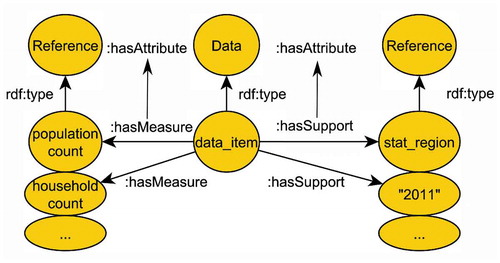
Figure 7. Ontology design pattern (OWL classes as boxes and properties as arrows) for capturing region attributes.

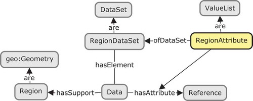
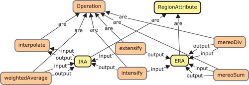
A region data set is a geodata set whose elements (data records) are supported by regions (polygon geometries). The latter is described in the GeoSPARQL ontology (prefix geo).¹⁴ In Figure 7, one can see how individual data items are linked to data sets as well as to attributes that describe their measured values. A region attribute is a list of such measures (ValueList) of a region data set (see Figure 7). The notion RegionAttribute, which is essential for this article, was defined in this vocabulary in terms of OWL axioms. IRAs and ERAs are subclasses of region attributes captured in the Extensive Measures ontology,¹⁵ which is illustrated in Figure 9 (compare Figure 8).

Figure 8. A computational diagram showing applicability of geospatial, arithmetic and mapping operations to extensive (ERA) and intensive region attributes (IRA) of different resolution. Blue boxes denote low resolution, orange boxes high resolution data.

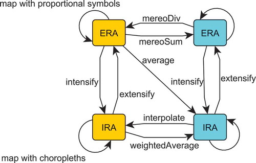
Figure 9. Ontology design pattern (OWL classes as boxes and properties as arrows) for capturing extensive and intensive region attributes with their admissible types of operations.

4.2. Operational constraints on IRA and ERA

How can we capture the constraints inherent in IRA and ERA with respect to GIS operations? We suggest the following kinds of arithmetic constraints:

1. Arithmetically speaking, weighted averages of the form:

(1) $measure(whl):=\frac{{\sum }_{p}size(support(p))\ast measure(p)}{{\sum }_{p}size(support(p))}$(1)

where p ranges over parts of a whole (whl) and weights are based on the support size of these parts (size(support(p))), are only applicable to intensive measures, while simple averages (where $weight=1$) are only meaningfully applicable to extensive measures. Examples for the latter are mean population counts over groups of countries or mean income over groups of persons. Examples for the former are the estimation of the sum GDP over several countries from the GDP per capita per country, or the computation of a temperature mean. At first, this rule may seem to contradict a common practice in climate science to simply average temperature measurements, even though they are intensive quantities.¹⁶ However, as argued in physics textbooks, a thermodynamically adequate temperature mean needs to take into account the size of the support for which the temperature holds (Hatsopoulos and Keenan 1965, Redlich 1970). For example, the masses of air around a temperature sensor influence measurement, and thus larger masses need to contribute more to an averaged temperature. Weighting temperature by mass implicitly turns it into its extensive thermodynamic equivalent, heat content (energy).¹⁷ This thermodynamic necessity may sometimes be numerically neglectable in practice when support sizes are homogeneous but becomes very apparent when the supports have very different sizes. Consider computing the average temperature of two large lakes, which clearly requires using an average weighted by volume.

• (2) The inverse operation to a weighted average, which disaggregates region attributes, is called interpolation. It is likewise only applicable to IRAs and corresponds to the problem of areal interpolation as understood in GIS (Figure 4(a)). Here, we assume a surface of intensive areal measures in space which can be sampled around a point in a continuous fashion, such as a mean income inside a spatial neighborhood.

• (3) Furthermore, mereological sums,¹⁸ i.e. arithmetic sums of region measures that are attributed to the merger of their regions

(2) $measure(whl):=\sum _{p}measure(p)\parallel \underset{p}{\cup }support(p)=support(whl)$(2)

require extensive measures. For example, when summing up population counts over administrative regions. This corresponds to the fact that it is meaningless to sum up ratios, or other extensive measures that do not add up to a mereological whole. More generally, one can ask whether arithmetic sums always require extensive measures. We suppose yes, but leave a definite answer of this question to a more in-depth ontological analysis of these operations.

• (4) The inverse operation, a mereological difference (mereoDiv), is likewise only applicable to extensive measures:

(3) $\begin{array}{c}measure(wh{l}_1\mathrm{\setminus }wh{l}_2):=measure(wh{l}_1)-measure(wh{l}_2)\parallel \\ support(wh{l}_1\mathrm{\setminus }wh{l}_2)=support(wh{l}_1)\mathrm{\setminus }support(wh{l}_2)\end{array}$(3)

This captures means of disaggregation such as area division with a known attribute value of a subarea. For example, knowing the population of a subarea allows us to compute the population of the remainder of a known area.

• (5) We call the construction of ratios with respect to a support size measure intensification of an extensive measure (e.g. density with respect to area size, and concentration with respect to mass or countable size), and the converse operation (multiplication of an intensive measure with some support size) extensification. Intensive measures can be derived using ratios of extensive measures (Canagaratna 1992),

  for example

(4) $measure(intensify(p)):=\frac{measure(p)}{size(support(p)}$(4)

These semantic constraints are summarized in a computational diagram Figure 8, forming a starting point for an algebra of operations on ERAs and IRAs. In this figure, orange boxes stand for data of higher resolution, while blue boxes stand for data of lower resolution. It can e.g. be seen that circumventing a mereological difference to turn an extensive measure into lower resolution data (in case corresponding data is not available) can be achieved through first intensifying ERA, then interpolating and extensifying the result (lower half of diagram). It is also noteworthy that averaging ERA is equivalent to building a mereological sum and intensifying the result, as can be seen by routing through the upper right corner in the diagram. Similarly, computing a weighted average of an IRA is nothing else than extensifying it and averaging the result (lower left corner). So this diagram allows us not only to identify possible computational paths but also equivalences among them. These constraints are captured by our pattern¹⁹ in terms of types of admissible GIS operations (see Figure 9).

4.3. Examples of labeled GIS tools

As a final step, we need to label concrete GIS operations with these types, in order to restrict their inputs and outputs and to match them with data. We illustrate this using software examples from ArcGIS.²⁰ To this end, subclasses of Operation²¹are used as labels to capture the semantics of GIS software tools in terms of the algebra (Section 4.2).

• The operation type interpolate can be used to describe ArcGIS’s Areal interpolation to polygons tool²² with the parameterizations Average (Gaussian) data (for field averages of a continuous variable) or Rate (binomial) counts (for population ratios) for IRAs, such as average temperature or unemployment rate.

  Interestingly, the alternative parametrization Event (overdispersed Poisson) counts of the same tool deal instead with ERAs (such as the number of whales observed by whale watchers in a standard interval). This parameterized tool can be annotated with an operation type that corresponds to the workflow chain: intensify $\circ$ interpolate $\circ$ extensify. As a matter of fact, a similar conversion workflow is implemented in this method internally (Krivoruchko et al. 2011).

• The operation type mereoSum can be used to describe ArcGIS’s Dissolve tool.²³ This tool dissolves a region layer into regions of lower resolution using a SUM statistic over a region attribute.

• The operation type mereoDiv can be used to describe ArcGIS’s Intersect tool with the Use Ratio Policy option.²⁴ With this option, a polygon which is the result of intersecting some region attribute with some intersect polygon obtains an attribute value which corresponds to the areal proportion of the input region attribute value.

• The weightedAverage operation type does not directly correspond to a tool in ArcGIS. However, it can be implemented by a ArcGIS workflow of the form: Create Field $\circ$ Field Calculator $\circ$ Summary Statistics to calculate an average over an area weighted attribute using the internal ‘area’ attribute of the region data set. According to Figure 8, weightedAverage also corresponds to a workflow of extensify $\circ$ mereoSum $\circ$ intensify.

• The operation types extensify and intensify can be used to describe standard operations using ArcGIS’s Field Calculator,²⁵ namely division by or multiplication with the predefined ‘area’ attribute of a region data set.

Apparently, there are many more example tools that would fit this scheme, and many more software packages for which such a labeling could be done (e.g. QGIS, Grass GIS etc., compare Ballatore et al. (2018)).

4.4. Discussion and outlook

As illustrated in Figure 2, once both tools and data sets are labeled with this vocabulary, it becomes possible to recommend data conversions and kinds of maps for region attributes in a given data set, as well as region attributes for a given GIS tool. The ontology proposed in this article adds an important semantic distinction to the rather superficial kind of information on data type and data formats that is usually available for such purposes (Hofer et al. 2017). For example, whether polygon vector data really represent extensive or intensive measures of an area or rather object outlines (of buildings, municipalities, a.s.o.) makes a large difference for statistical analysis. It now becomes possible to compare socio-demographic ratios (such as per capita income or health statistics) across various statistical data sources and regional levels, without a human interpreter needed who first checks which kinds of conversions are necessary to turn extensive into intensive measures. This leads us one step closer to a fully automatized statistics portals, where statistical data can be automatically converted into a form that is useful for answering analytic questions and for automatic mapping (Tomko et al. 2012, Scheider and Tomko 2016). Furthermore, a semantic workflow construction/reasoning tool which can deal with semantic types (Lamprecht 2013) could make use of these annotations to automatically construct meaningful workflows which lead from a given input to a given output type. In this way, we might be able in the future to ask a GIS to figure out on its own how we get from data about household counts and amounts of energy to a summary statistics about energy efficiency across regions. Finally, the ontology can also be used to do inference, e.g. to enrich data descriptions by propagating semantic information through a workflow in which labeled GIS methods are used, similar to Scheider and Ballatore (2017). This might be also a way to add semantic labels when data sets are not available for analysis but only workflows.

To realize such a linked workflow and analytical infrastructure, future work should address the following problems:

1. The classifier in Section 3.6 should be further evaluated and applied to various standard geodata sources on the Web, adding region attribute labels from our pattern.

2. Standard GIS tools and algebra operations should be annotated either on atomic levels or on the level of operational chains, as shown above. It should be investigated how to deal with parameters of tools which modify their semantic constraints, and how reasoning can deal with chains instead of atomic operations.

3. Cartographic tools and cartographic standard procedures should be labeled with operations and attribute types as in our proposed algebra.

4. It should then be tested how workflow composition, Web mapping and statistical portals can benefit from the proposed concepts, both in terms of complexity reduction and quality improvement.

5. The algebra introduced in Section 4.2 should be rigorously formalized and tested with Semantic Web reasoners, to generalize search over tools and region data sets.

5. Conclusion

The distinction between extensive and intensive properties, originating in Physics and Chemistry, was adopted in GIScience some time ago. While the importance of intensive and extensive properties has been acknowledged, a computable account of this distinction is still lacking. Yet, the notion is central for many theoretical and practical cartographic and geocomputational tasks, including the choice of map types suitable for visualizing region data, and how regions can be summarized and divided. We believe it has an important role to play in future semantic retrieval and workflow construction systems.

In this article, we analyzed this role in some depth for both Cartography and geocomputational tasks. We then tested the possibility of automatic labeling of such attributes in region geodata sets using a range of ML classifiers based on features readily extractable from geodata files. Since region data sets are not merely random area samples of a continuous spatial field, classifiers need to go beyond simple correlation measures. We found that on our tested data set of 519 statistical attributes from CBS, the SVM RBF classifier performed with very high accuracy both on balanced and unbalanced samples, and that the most important predictors were the intercept of the regression line for the measure/area plot, as well as the Getis–Ord G statistic. We further argued that this result fits well into our understanding of intensive and extensive properties although further tests are necessary for different samples of statistical regions and different locations. Finally, we illustrated how this classifier could be used for meaningful computation and mapping. We suggested an algebraic sketch and a corresponding ontology design pattern for annotating geodata and GIS tools and for reasoning with intensive and ERAs when using GIS operations. We demonstrated that such a labeling can be done using many example operations from ArcGIS. In future work, it should be tested to what extent statistical portals and workflow composition can benefit from a linked data infrastructure which exploits automated semantic labeling, automated data conversions and maps. Finally, we believe that the proposed algebra could form a part of a larger theory of meaningful geocomputation, where extensive and intensive properties may add to the current set of spatial core concepts (Kuhn 2012).

Acknowledgments

We would like to thank Tom de Jong for making us aware of the cartographic constraints of intensive and extensive properties. Furthermore, we have to thank our anonymous reviewers for many valuable suggestions, especially regarding some of the illustrative examples.

Disclosure statement

No potential conflict of interest was reported by the authors.

Additional information

Notes on contributors

Simon Scheider

Simon Scheider is an assistant professor in geographic information science at the Department of Human Geography and Planning. His research lies at the interface between conceptual modeling, geographic data analysis and knowledge extraction.

Mark D. Huisjes

Mark D. Huisjes is a student of Human Geography at the Department of Human  Geography and Planning.

Notes

1. The distinction is implicitly reflected e.g. in Monmonier’s discussion on data maps (ch. 10) (Monmonier 2014) and in Kraak and Ormeling (2011)’s account of choropleth mapping.

2. http://pro.arcgis.com/en/pro-app/tool-reference/data-management/resample.htm

3. http://www.geography.hunter.cuny.edu/˜jochen/GTECH361/lectures/lecture10/concepts/05%20-%20Split%20and%20merge%20policies.htm

4. Compare chapter 2 in Chrisman (1997).

5. The problem of estimating a single label for each region attribute.

6. https://github.com/MarkHuisjes/Checker/blob/master/TensityChecker.py

7. https://www.cbs.nl/nl-nl/maatwerk/2016/30/kerncijfers-wijken-en-buurten-2016

8. See https://github.com/MarkHuisjes/Checker/blob/master/TensityChecker.py

9. http://desktop.arcgis.com/en/arcmap/latest/manage-data/tables/calculating-area-length-and-other-geometric-properties.htm

10. desktop.arcgis.com/en/arcmap/10.3/tools/data-management-toolbox/project.htm

11. https://github.com/rkern/line_profiler

12. http://geographicknowledge.de/vocab/AnalysisData.rdf

13. Web Ontology Language (https://www.w3.org/TR/owl-overview/)

14. http://www.opengis.net/ont/geosparql

15. http://geographicknowledge.de/vocab/ExtensiveMeasures.rdf

16. https://www.carbonbrief.org/explainer-how-do-scientists-measure-global-temperature

17. See e.g. https://chiefio.wordpress.com/2011/07/01/intrinsic-extrinsic-intensive-extensive/.

18. A mereological sum, in its purely logical definition, is a way to talk about wholes and parts in a formal way (Casati and Varzi 1999). We use this term here to denote specific arithmetic sums and differences, namely ones that involve also a merger or division of the supporting spatial regions.

19. http://geographicknowledge.de/vocab/ExtensiveMeasures.rdf

20. https://www.arcgis.com

21. From the workflow ontology http://geographicknowledge.de/vocab/Workflow.rdf, see Scheider and Ballatore(2017).

22. https://desktop.arcgis.com/en/arcmap/latest/tools/geostatistical-analyst-toolbox/areal-interpolation-layer-to-polygons.htm

23. http://desktop.arcgis.com/de/arcmap/10.3/tools/data-management-toolbox/dissolve.htm

24. http://desktop.arcgis.com/en/arcmap/10.3/tools/analysis-toolbox/intersect.htm

25. desktop.arcgis.com/en/arcmap/10.3/tools/data-management-toolbox/calculate-field.htm

References

- Alper, P., et al., 2015. Labelflow: exploiting workflow provenance to surface scientific data provenance. In: B. Ludaescher and B. Plale, eds. Provenance and annotation of data and processes. 5th. International Provenance and Annotation Workshop Springer, 84–96.
- Ballatore, A., Scheider, S., and Lemmens, R., 2018. Patterns of consumption and connectedness in GIS web sources. In: The Annual International Conference on Geographic Information Science Springer, 129–148.
- Bernard, L., et al., 2014. Scientific geodata infrastructures: challenges, approaches and directions. International Journal of Digital Earth, 7 (7), 613–633. doi:10.1080/17538947.2013.781244
- Bertin, J., Barbut, M. and Bonin, S. ... (1967). Sémiologie graphique: les diagrammes, les réseaux, les cartes. Paris/La Haye: Gauthier-Villars/Mouton
- Bizer, C., Heath, T., and Berners-Lee, T., 2009. Linked data-the story so far. International Journal on Semantic Web and Information Systems, 5 (3), 1–22.
- Bobat, A., 2015. Thermal pollution caused by hydropower plants. In: A.N. Bilge, A.Ö. Toy, and M.E. Günay, eds. Energy systems and management. Cham: Springer International Publishing, 19–32.
- Buchanan, I. and Lambert, G., 2005. Deleuze and space. Toronto: University of Toronto Press.
- Burrough, P.A., 1986. Principles of geographical information systems for land resources assessment. New York: Oxford University Press.
- Canagaratna, S.G., 1992. Intensive and extensive: underused concepts. Journal Chemical Education, 69 (12), 957. doi:10.1021/ed069p957
- Carral, D., et al., 2013. An ontology design pattern for cartographic map scaling. In: Extended Semantic Web Conference Berlin, Heidelberg : Springer, 76–93.
- Casati, R. and Varzi, A.C., 1999. Parts and places: the structures of spatial representation. Cambridge, MA: MIT Press.
- CBS, 2014. Kerncijfers wijken en buurten 2014. [online]. Available from: https://www.cbs.nl/nl-nl/maatwerk/2015/48/kerncijfers-wijken-en-buurten-2014 [Accessed May 2017].
- Chrisman, N., 1997. Exploring geographic information systems. Washington: Jon Wiley & Sons.
- Cohen, E.R., 2007. Quantities, units and symbols in physical chemistry. Cambridge, UK: Royal Society of Chemistry.
- De Smith, M.J., Goodchild, M.F., and Longley, P., 2007. Geospatial analysis: a comprehensive guide to principles, techniques and software tools. Leicester, UK: Troubador Publishing Ltd.
- Deleuze, G., 1994. Difference and repetition. New York: Columbia University Press.
- Egenhofer, M.J., 2002. Toward the semantic geospatial web. In: Proceedings of the 10th ACM international symposium on Advances in geographic information systems, 1–4. doi:10.1044/1059-0889(2002/er01)
- Evans, I.S., 1977. The selection of class intervals. Transactions of the Institute of British Geographers, 2, 98–124. doi:10.2307/622195
- Flowerdew, R. and Green, M., 1993. Developments in areal interpolation methods and GIS. In: M.M. Fischer and P. Nijkamp, eds. Geographic information systems, spatial modelling and policy evaluation. Berlin, DE: Springer, 73–84.
- Fotheringham, A.S. and Wong, D.W., 1991. The modifiable areal unit problem in multivariate statistical analysis. Environment and Planning A, 23 (7), 1025–1044. doi:10.1068/a231025
- Friedman, J., Hastie, T., and Tibshirani, R., 2001. The elements of statistical learning. Vol. 1, New York,NY: Springer series in statistics.
- Gangemi, A. and Presutti, V., 2010. Ontology design patterns. In: S. Staab and R. Studer, eds. Handbook on ontologies. Dordrecht: Springer Science & Business Media.
- Goodchild, M.F. and Lam, N.S.N., 1980. Areal interpolation: a variant of the traditional spatial problem. London, ON, Canada: Department of Geography, University of Western Ontario.
- Goodchild, M.F., Yuan, M., and Cova, T.J., 2007. Towards a general theory of geographic representation in GIS. International Journal of Geographical Information Science, 21 (3), 239–260. doi:10.1080/13658810600965271
- Gorenstein, M. and Gadzicki, M., 2011. Strongly intensive quantities. Physical Review C, 84 (1), 1–5. doi:10.1103/PhysRevC.84.014904
- Hatsopoulos, G.N. and Keenan, J.H., 1965. Principles of general thermodynamics. Vol. 398, New York,NL: Wiley.
- Hofer, B., et al. 2017. Towards a knowledge base to support geoprocessing workflow development. International Journal of Geographical Information Science, 31 (4), 694–716. doi:10.1080/13658816.2016.1227441
- Huang, W., et al. 2018. Synchronising geometric representations for map mashups using relative positioning and linked data. International Journal of Geographical Information Science, 32 (6), 1117–1137. doi:10.1080/13658816.2018.1441416
- Jaeger, J.A., 2000. Landscape division, splitting index, and effective mesh size: new measures of landscape fragmentation. Landscape Ecology, 15 (2), 115–130. doi:10.1023/A:1008129329289
- Janowicz, K., Scheider, S., and Adams, B., 2013. A geo-semantics flyby. In: S. Rudolph, et al., eds. Reasoning web. semantic technologies for intelligent data access. Vol. 8067. Dordrecht: Springer, 230–250.
- Jelinski, D.E. and Wu, J., 1996. The modifiable areal unit problem and implications for landscape ecology. Landscape Ecology, 11 (3), 129–140. doi:10.1007/BF02447512
- Jones, C.B., 2014. Geographical information systems and computer cartography. London: Routledge.
- Kemp, K., 2007. Encyclopedia of geographic information science. Los Angeles: SAGE publications.
- Kraak, M.J. and Ormeling, F., 2011. Cartography: visualization of spatial data. New York: Guilford Press.
- Krivoruchko, K., Gribov, A., and Krause, E., 2011. Multivariate areal interpolation for continuous and count data. Procedia Environmental Sciences, 3, 14–19. doi:10.1016/j.proenv.2011.02.004
- Kuhn, W., 2012. Core concepts of spatial information for transdisciplinary research. International Journal of Geographical Information Science, 26 (12), 2267–2276. doi:10.1080/13658816.2012.722637
- Kyriakidis, P., 2017. Aggregate data: geostatistical solutions for reconstructing attribute surfaces. In: X.Z. Shashi Shekhar and H. Xiong, eds. Encyclopedia of GIS. chap. 7. New York,NY: Springer, 57–67.
- Lamprecht, A.L., 2013. User-level workflow design. Lecture Notes in Computer Science, 8311. Berlin: Springer.
- Learn, S., 2017. SVM documentation. [online]. Available from: http://scikit-learn.org/stable/modules/generated/sklearn.svm.SVC.html [Accessed May 2017].
- Lin, J., Hanink, D.M., and Cromley, R.G., 2017. A cartographic modeling approach to isopleth mapping. International Journal of Geographical Information Science, 31 (5), 849–866. doi:10.1080/13658816.2016.1207776
- Lobato, J. and Thanheiser, E., 1999. Re-thinking slope from quantitative and phenomenological perspectives. In: Proceedings of the 21st Annual Meeting of the North American Chapter of the International Group for the Psychology of Mathematics Education, Vol. 1, 291–297.
- Longley, P.A., et al., 2005. Geographic information systems and science. Chichester, UK: John Wiley & Sons.
- McNaught, A.D. and McNaught, A.D., 1997. Compendium of chemical terminology. Vol. 1669. Oxford, UK: Blackwell Science Oxford.
- Mijnarends, R., et al., 2015. Advanced data-driven performance analysis for mature waterfloods. In: SPE Annual Technical Conference and Exhibition. Society of Petroleum Engineers.
- Monmonier, M., 2014. How to lie with maps. Chicago: University of Chicago Press.
- Müller, J.C., Lagrange, L.P., and Weibel, R., 1995. GIS and generalization: methodology and practice. London: Taylor & Francis.
- Openshaw, S., 1984a. Ecological fallacies and the analysis of areal census data. Environment and Planning A, 16 (1), 17–31. doi:10.1068/a160017
- Openshaw, S., 1984b. The modifiable areal unit problem. In: No. 38 concepts and techniques in modern geography. Norwich, UK: Geo Books.
- Pedregosa, F., et al. 2011. Scikit-learn: machine learning in python. Journal of Machine Learning Research, 12, 2825–2830.
- Redlich, O., 1970. Intensive and extensive properties. Journal Chemical Education, 47 (2), 154. doi:10.1021/ed047p154.2
- Scheider, S. and Ballatore, A., 2017. Semantic typing of linked geoprocessing workflows. International Journal of Digital Earth, 11 (1), 113–138.
- Scheider, S., Ostermann, F.O., and Adams, B., 2017. Why good data analysts need to be critical synthesists. determining the role of semantics in data analysis. Future Generation Computer Systems, 72, 11–22. doi:10.1016/j.future.2017.02.046
- Scheider, S. and Tomko, M., 2016. Knowing whether spatio-temporal analysis procedures are applicable to datasets. In: R. Ferrario and W. Kuhn, eds. Formal ontology in information systems. Amsterdam: Frontiers in Artificial Intelligence and Applications IOS Press, 67–80.
- She, B., Duque, J.C., and Ye, X., 2017. The network-Max-P-regions model. International Journal of Geographical Information Science, 31 (5), 962–981. doi:10.1080/13658816.2016.1252987
- Stasch, C., et al., 2014. Meaningful spatial prediction and aggregation. Environmental Modelling & Software, 51, 149–165. doi:10.1016/j.envsoft.2013.09.006
- Stern, C. and Sester, M., 2013. Deriving constraints for the integration and generalization of detailed environmental spatial data in maps of small scales. In: Proceedings of the 16th ICA Workshop on Generalisation and Multiple Representation, jointly organised with the ICA Commission on Map production and Geo-Business, 23–24.
- Stevens, J., 2016. Earth Observatory images by Joshua Stevens, using Suomi NPP VIIRS data from Miguel Romàn, NASA’s Goddard Space Flight Center. [online]. NASA, Available from: https://earthobservatory.nasa.gov/Features/NightLights/ [Accessed January 2017].
- Suppes, P. and Zinnes, J.L., 1963. Basic measurement theory. In: D. Luce et al, eds. Handbook of mathematical psychology, Volume I. New York: John Wiley & Sons, 1–76.
- Tolman, R., 1917. The measurable quantities of physics. Physical Review, 9 (3), 237–253.
- Tomko, M., et al., 2012. The design of a flexible web-based analytical platform for urban research. In: I. C. et al., ed. Proceedings of the 20th international conference on advances in geographic information systems, 369–375.
- Tooamnian, A., et al., 2013. Automatic integration of spatial data in viewing services. Journal of Spatial Information Science, 2013 (6), 43–58.
- US Census Bureau, 2017. Annual estimates of the resident population for the United States, regions, states, and puerto rico: april 1, 2010 to July 1, 2016. [online]. Available from: https://www2.census.gov/programs-surveys/popest/datasets/2010-2016/national/totals/nst-est2016-alldata.csv [Accessed June 2017].