Fine-grained landuse characterization using ground-based pictures: a deep learning solution based on globally available data

ABSTRACT

We study the problem of landuse characterization at the urban-object level using deep learning algorithms. Traditionally, this task is performed by surveys or manual photo interpretation, which are expensive and difficult to update regularly. We seek to characterize usages at the single object level and to differentiate classes such as educational institutes, hospitals and religious places by visual cues contained in side-view pictures from Google Street View (GSV). These pictures provide geo-referenced information not only about the material composition of the objects but also about their actual usage, which otherwise is difficult to capture using other classical sources of data such as aerial imagery. Since the GSV database is regularly updated, this allows to consequently update the landuse maps, at lower costs than those of authoritative surveys. Because every urban-object is imaged from a number of viewpoints with street-level pictures, we propose a deep-learning based architecture that accepts arbitrary number of GSV pictures to predict the fine-grained landuse classes at the object level. These classes are taken from OpenStreetMap. A quantitative evaluation of the area of Île-de-France, France shows that our model outperforms other deep learning-based methods, making it a suitable alternative to manual landuse characterization.

KEYWORDS:

• Landuse characterization
• convolutional neural networks
• ground-based pictures
• volunteered geographic information
• urban areas

1. Introduction and related work

According to the UN’s report ‘The Worlds Cities in 2016’,¹ the population living in urban areas will rise from 4.034 billion in 2016 to a projected 5.058 billion in 2030. Therefore, 60% of the world’s population will be likely residing in cities by 2030. As the number of people living in urban environments increases, gathering information about existing infrastructure and landuse becomes very important, both for the maintenance of existing urban spaces and the planning of future ones. Moreover, cities are dynamic, leading to an increased demand for landuse monitoring that is both up-to-date and accurate. By landuse, we consider how a space, generally man-made, is being utilized by humans, for example, as a hospital, a school, a museum, or a park. Traditionally, landuse mapping has been performed with the help of field surveys. Authoritative surveys are expensive and time-consuming, as they require massive human intervention in almost all steps. It is also unpractical to update such maps on a frequent basis. For all these reasons, one would want to automatize the process using a data-driven approach.

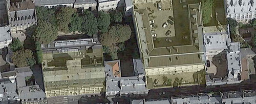
A task related to landuse characterization is landcover mapping (i.e. characterization of materials at the ground level), which in the last decade has seen a rising number of researches using remote sensing-based approaches (Homer et al. 2015, Postadjiana et al. 2017). While identifying different types of landcover classes based on their respective spectral signatures is possible, it is much harder to extract landuse related information from image bands, as the spectral information from the overhead imagery is not sufficient to differentiate the same (landcover) materials into different landuse classes. For example, a concrete building could belong to a school, a town hall, or a hospital (Figure 1).

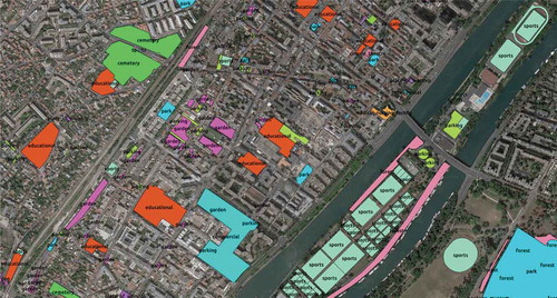
Figure 1. The highlighted building on the left is an educational institute and the one on the right is a government building. These two classes could be difficult to distinguish using only remotely sensed imagery. Source: Imagery from Google Maps of an area in the city of Paris.

Also, a landuse class is often composed of a series of objects, possibly made of different materials. For example, a hospital could enclose a park, roads and buildings within its boundaries. For these reasons, obtaining accurate landuse maps at the urban-object level from imagery (top-view) alone is challenging.² If recent remote sensing-based research has considered image textures and context to circumvent this problem (Pacifici et al. 2009, Tuia et al. 2015), it makes the assumption that different types of landuse show different morphological structures when seen from above.

To cope with these shortcomings, recent research has started utilizing geo-referenced ground-based pictures repositories as alternative data sources for characterizing land usages (Lefevre et al. 2017). Authors in Tracewski et al. 2017 use geo-tagged pictures available on social media (e.g. Flickr, Instagram) and online picture repositories (e.g. Geograph) to map landcover for the cities of London, United Kingdom and Paris, France. Authors of Zhou et al. (2014) studied the possibility of recognizing characteristic features of cities using geo-referenced pictures from the (now discontinued) social media platform Panoramio. Another study using Panoramio (Produit et al. 2014a), where authors considered the geographical conditions that make a location good to take an appealing picture. However, the use of ground-based pictures from social media raises a number of concerns such as:

1. Often, the content of the pictures does not point to the specific urban-object at that geo-localization. Pictures of social media being subjective in nature, they represent the perception of the user holding the camera and generally include far away touristic viewpoints, landscapes, or other unwanted content (from a landuse mapping perspective) such as selfies, macros of flowers or pets.

2. The distribution of pictures across the city is uneven: while touristic locations are often pictured, less frequented but important urban-objects like hospitals, government buildings or industry tend to be not proportionately represented in the user-generated content.

3. The accuracy of the geo-tags is variable because many pictures either lack metadata about the orientation and position of the camera or the geolocalization is inaccurate since entered directly by the user by clicking on a map with an inadequate zoom level (Produit et al. 2014b).

4. Depending on the source, the data is not densely available for many cities around the globe. For example, Geograph has a collection of images representative of $1km\times 1km$ grid square, which is quite sparse for the task of landuse mapping at urban-object level. It also is geographically limited to Great Britain, Ireland, and the Isle of Man.

For all these reasons, we consider an alternative source of ground-based pictures that is widely available, covers most urban-objects and is constantly updated: Google Street View (GSV). These pictures have the advantage of providing panoramic views along most streets in cities (in 2012, 39 countries with 3000 cities were already covered).³ GSV pictures can be downloaded via the GSV API.⁴ These accurately geo-referenced ground pictures objectively capture urban-objects, offering as well the possibility of multiple zoom levels. Some of the privacy issues are addressed by blurring faces, number plates, and house numbers. ⁵ In the last couple of years, researchers have started using GSV pictures to assess physical changes in urban areas (Naik et al. 2017), to catalog urban trees (Wegner et al. 2016), or to classify storefronts into types of shops (Movshovitz-Attias et al. 2015). Other works have used GSV pictures for understanding the socioeconomic attributes of areas in various US cities (Gebru et al. 2017) or for finding characteristic visual elements that distinguish European cities (Doersch et al. 2012).

Lately, researchers have also started to use GSV pictures for landuse characterization. For example (Workman et al. 2017) propose a methodology to use GSV pictures along with dense (public) ground truth annotations provided by the New York City Department of City Planning; with this data, they train a model predicting landuse at the pixel level for New York. Despite the impressive results, the method cannot easily be applied to other cities, as most do not have such high quality pre-processed labels. Furthermore, direct generalization to other cities seems unlikely because of inter-city domain adaptation problems (Chen et al. 2017). Finally, this kind of ground truth is not frequently updated because of economic reasons, availability of experts, time and efforts involved.

To tackle these issues we propose to train our landuse characterization models with ground labels extracted from an open, widely available data source: OpenStreetMap (OSM).⁶ OSM is an open and collaborative geographic data platform which provides labels for various urban-objects in cities worldwide. Using OSM as a data source, allows us: (i) to retrieve annotations for a large number of urban-objects and, (ii) to design a methodology that can be applied to many cities worldwide.

To summarize, in this paper we propose a model to exploit ground-based pictures from GSV and labels from OSM to characterize landuse at the urban-object level. Following the great success of deep learning methods (Goodfellow et al. 2016) in several data processing tasks (including those described above and general landcover/landuse mapping (Zhu et al. 2017)), we adopt a convolutional neural network (CNN) strategy, where the model is trained using the GSV pictures pertaining to an urban-object and the corresponding landuse class extracted from OSM. While CNNs have been used in other recent works aiming at urban landuse characterization (Workman et al. 2017, Zhu et al. 2018), we propose a method that exploits data coming from multiple views: given that a series of ground-based pictures are available to capture several views of the same urban-object, our proposed model combines features extracted from all the available ground images into a single representation, which is then used to predict the urban-object label in a common trunk of the network. Our model is inspired by Siamese Neural Networks (Bromley et al. 1994), and in particular, by the recent TI-Pooling model proposed to deal with rotation invariance (Laptev et al. 2016). With respect to the latter, our model called Variable Input Siamese Convolutional Neural Network (VIS-CNN) accepts a variable number of images corresponding to the number of GSV pictures available for the urban-objects and aggregates them to learn the urban-object categorization in an end-to-end manner.

The rest of the paper is as follows: our VIS-CNN method is explained in section 2 while the creation of the dataset is presented in section 3. Experimental results are shown in section 4 and discussed in section 5.

2. Model

2.1. CNNs for classification

Compared to other traditional machine learning algorithms, CNNs are unique since they perform feature extraction and classification jointly, that is, they learn both the image representation (the features) and the decision function (the classifier) performing the image recognition. A complete introduction to CNNs is beyond the scope of this paper, but the interested readers can find comprehensive information in the book by Goodfellow et al. (2016). In the following, we present the necessary concepts to understand our proposed Siamese architecture, described in subsection 2.2.

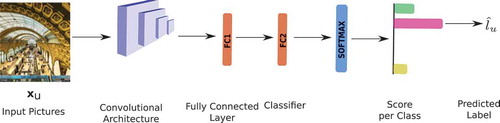
A standard pipeline for classification with CNN models is shown in Figure 2. CNNs are composed of a series of operations called convolutions: a convolution is a linear and local operator in which we compute the scalar product between a $mxm$ filter and each $mxm$ overlapping neighborhood in the input image, producing the so-called activation map. The convolution filter is then applied to the image as a sliding window, therefore providing an activation map. Since the same filter is applied all over the image, we say that such filter is shared spatially: this is one of the keys of the success of CNNs, as the number of parameters to be learned (corresponding to each cell of the convolution filters in the network) is greatly reduced.

Figure 2. Standard CNN Model for classification. Predicting one category per picture.

The convolution is a linear operator. Thus, a composition of multiple convolutions is also a linear operator. To allow such composition to provide a richer representation of the image data, capable of learning more complex patterns, a non-linear function is generally applied to each activation map. The nonlinearity that we use in this paper is called Rectified Linear Units (ReLU) (Nair and Hinton 2010) and corresponds to a gating function returning the activation value when it is positive and zero otherwise.

After the convolution and the nonlinearity, a stage of spatial reduction is also generally applied. Such spatial reduction, called pooling, downsamples the activation map and allows the model to recognize objects independently from their relative location in the image. Traditional pooling strategies involve max-pooling (taking the maximum in a $p\times p$ spatial window of the activation map) or average pooling (taking the average).

Convolutions, nonlinearity, and pooling are the three main components of a CNN block whose output is then fed as an input to the next block. In Figure 2, convolutional blocks are represented by purple parallelepipeds. As a direct consequence, the next range of convolutional filters will ‘see’ a wider part of the image (since the image has been downsampled) and will also recombine information coming from the previous layers: by doing so, the filters extracted become more and more semantic, that is, they represent characteristics specific of the class being observed (Zeiler and Fergus 2014). Each block is made up of several learnable filters and the number of convolutional blocks defines the ‘depth’ of a CNN.

The input picture undergoes a series of blocks of convolutions, nonlinearity and pooling operators resulting in a downsampled activation map. Afterward, fully connected layer(s) is(are) used to transform this activation map into a high-dimensional feature vector that can be fed to any classifier.

In Figure 2, fully connected layers are represented by orange blocks. For an input picture fed to the CNN block, we get an activation map which is transformed by the first fully connected layer (FC1) into a high-dimensional feature vector. CNNs for classification use the output of FC1 to learn a classifier (also a fully connected layer, FC2 in Figure 2) solving the task at hand (in our case, discriminating among different landuse classes). This fully connected layer is followed by a softmax operation (in blue in Figure 2) which is often used to convert the output of the classifier into scores between $[0,1]$ and summing to one. The class with the maximum score is the final predicted label.

During the training phase, a CNN learns all its parameters. This is done in CNNs by backpropagation: first a set of previously annotated samples is passed through the network (feed-forward pass) to obtain their classifications. A loss is then computed, using the classifications provided by the network and the ground truth labels of the samples. The loss is then backpropagated by computing its gradient with respect to the network parameters and updating them in the direction that corresponds to the maximum decrease of the empirical loss.

2.2. Proposed Siamese-like architecture

Our objective is to predict the class $l_u\in [1,...,K]$ of a given urban-object $u$, where $K$ is the number of classes. To obtain the classification for the urban-object $u$, we use a collection of $N_u$ pictures of this urban-object: ${\left\{{\mathbf{x}}_u^i\right\}}_{i=1}^{N_u}$.

These pictures capture different views of the urban-object and lead to a more descriptive representation of the urban-object as a whole. Our approach is to use each of these different pictures as an input to a CNN and then combine their feature vectors to learn a single classifier accounting for all of the pictures simultaneously. To this end, we use a Siamese Network (Bromley et al. 1994) but customized to accommodate a variable number of input images per object being predicted. A schematic representation of our model is shown in Figure 3.

Figure 3. Proposed VIS-CNN model. The GSV pictures for an urban-object $u$ are fed to a pre-trained network to give an activation vector $\mathbf{f}({\mathbf{x}}_u)$ per picture. Each activation vector is obtained as an output of the last fully connected layer of the CNN model (orange blocks). The resulting activation map is then flattened to give high-dimensional activation vector $\mathbf{g}(u)$, which is fed to the second stage leading to the prediction ${\hat{l}}_u$.

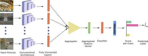
The convolutional part of the network (purple parallelepipeds) together with the fully connected layers (orange blocks) extract features from each image separately (see Figure 3). Note that we use the same network model (VGG16 (Simonyan and Zisserman 2014), pre-trained on the ImageNet database) to extract a feature vector from each image. In general, training a CNN model with millions of parameters requires a large amount of annotated data. Since we have a limited amount of data thus it is beneficial to use a pre-trained network, already trained for object recognition with a multi-million images dataset. Further, we fine-tune this pre-trained model with our dataset for the task of landuse classification. Proceeding this way, we diminish the risk of overfitting and also make the whole model trainable. Using this standard architecture, we extracted a set of $N_u$ feature vectors, $\mathbf{f}({\mathbf{x}}_u^i)$ one per each picture $i$ pertaining to urban-object $u$. Once the feature vectors $\mathbf{f}({\mathbf{x}}_u^i)$ are extracted for each image, we need to aggregate them to obtain a fixed-size vector that can be used as an input to the second part of the network that performs landuse classification based on the ensemble of pictures. To this end, we test two aggregators, inspired by spatial pooling strategies:

(1) $g(u{)}_{\mathrm{m}\mathrm{a}\mathrm{x}}^j=\underset{i}{max}f({\mathbf{x}}_u^i{)}^j,$(1)

(2) $g(u{)}_{\mathrm{a}\mathrm{v}\mathrm{g}}^j=\frac{1}{N_u}\sum _{i=1}^{N_u}f({\mathbf{x}}_u^i{)}^j,$(2)

where $f(\cdot {)}^j$ represents the $j^{th}$ element of vector $\mathbf{f}(\cdot )$. These two strategies lead to different interpretations of the data fusion:

– When using the MAX aggregator, one assumes that for every neuron in the fully connected layers, there is one image carrying the most discriminative information. In this sense, the CNN is performing inputs selection and picks the most important representation in a picture-wise manner per neuron.

– When using the AVG aggregator, the CNN summarizes all the images into average descriptors avoiding the kind of specialization described in the case of MAX aggregator. The average thus gives more importance to the most repeated attributes appearing in the ensemble of pictures associated with a given urban-object.

The aggregated feature vector $\mathbf{g}(u)$ is then used as an input to the final fully-connected classifier layer which maps the aggregated feature vector to the class of interest. As for a standard CNN, the softmax function is used to obtain the predicted class $\widehat{l_u}$ of the urban-object $u$ Figure 3). In our proposed VIS-CNN, all the parameters for both the convolutional and fully-connected layers are learned end-to-end. Therefore, for this classification task, we use a database of $N$ urban-objects that have been annotated (with classes $\left\{l_1,\dots ,l_N\right\}$) and their associated pictures sets $\left\{{\mathbf{x}}_1,\dots ,{\mathbf{x}}_N\right\}$. Note that every urban-object ${\mathbf{x}}_u$ is observed through a series of GSV pictures ${\left\{{\mathbf{x}}_u^i\right\}}_{i=1}^{N_u}$. The extraction of this database is discussed in section 3. We use the cross-entropy as a loss function:

(3) $L=\frac{1}{N}\sum _{u=1}^N\left[-\sigma (\widehat{l_u}=l_u|{\mathbf{x}}_u^1,\dots ,{\mathbf{x}}_u^{N_u})+log\left(\sum _{k=1}^{K}exp(\sigma (\widehat{l_u}=k|{\mathbf{x}}_u^1,\dots ,{\mathbf{x}}_u^{N_u}))\right)\right],$(3)

where $\sigma (\widehat{l_u}=k|{\mathbf{x}}_u^1,\dots ,{\mathbf{x}}_u^{N_u})$ is the softmax score given by the model for the urban-object $u$ and class $k$.

When using $\mathbf{g}(u{)}_{\mathrm{m}\mathrm{a}\mathrm{x}}$ (respectively $\mathbf{g}(u{)}_{\mathrm{a}\mathrm{v}\mathrm{g}}$), the aggregation step can be seen as a max (respectively, average) pooling on the different branches of the network pertaining to the single pictures. This allows updating the network parameters in a single backward pass. For this reason, we can use the same gradient backpropagation rules used in spatial pooling but applied picture-wise.

3. Dataset

We apply the proposed neural network to urban-objects dataset taken from the region of Île-de-France, France. For creating our urban-objects dataset we considered the metropolitan area of Paris and nearby suburbs including Versailles, Orsay, Orly, Aulnay-sous-Bois, Le Bourget, Sarcelles, Chatou and Nanterre enclosed within the region of Île-de-France. Since our proposed model is supervised, we need to obtain training data composed of a set of pictures per urban-object and their corresponding true labels. In the following, we detail the data collection procedure applied in this study.

3.1. Landuse footprints and annotations from OSM

To obtain the collection of urban-objects we used OSM. The OSM database contains a large variety of landuse categories from which we selected 16 classes (Table 1). After grouping the volunteer assigned labels into our selected $16$ landuse labels, we extracted all spatial footprints as polygon shapes and the corresponding label (Figure 4).

Table 1. Urban-objects dataset in Île-de-France, France.

			% Urban-Objects with #pictures in range of:
Landuse class	# OSM objects	# GSV pictures	1–8	9–16	17+
Educational	500	2970	81	14	5
Hospital	168	2102	51	26	23
Religious	500	2431	89	6	5
Shop	333	2606	71	17	12
Cemetery	259	2189	62	26	12
Forest	500	6476	63	18	19
Park	999	7477	77	14	9
Heritage	117	1948	59	15	26
Sports	500	1772	90	7	3
Government	500	2875	85	7	8
Post Office	108	329	99	0	1
Parking	500	2414	85	10	5
Fuel	152	416	94	4	2
Marina	43	1350	21	16	63
Hotel	423	2304	84	9	7
Industrial	339	5298	60	14	26
Total	5941	44957

Figure 4. Examples of polygon footprints and labels extracted from OSM.

To do so we looked for polygons which had an entry in the name column (in OSM shape layer attribute table). We then queried certain keywords (from a ‘keyword and corresponding landuse’ dictionary that we handcrafted) in the name column entry. These keywords generally are descriptive of the landuse class which we have designed. For example, the words ‘Lycée’ or ‘Ecole’ (respectively, “high-school’’ and “school’’ in French) correspond to the landuse ‘school’ in our keywords dictionary. Then, we searched again in the attribute table all the polygons with missing name column entry but with a unique volunteer assigned label in other columns. In total, 5941 urban-objects were gathered, whose class distribution is summarized in Table 1.

3.2. Pictures collected from GSV

For every urban-object, we downloaded two sets of pictures from GSV using the Google API (see Figure 5 for an example):

Figure 5. (a) Google Street View Pictures for an Urban-Object from outside location, (b) Labels from OpenStreetMap for the same Urban-Object, (c) Google Street View Pictures for an Urban-Object from inside location.

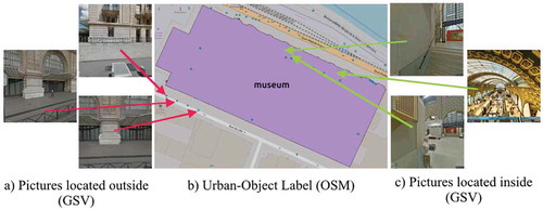
– Pictures located on streets surrounding the urban-object and looking towards it. In this case, we selected the roads nearest to the object (within a maximum distance of 12 meters from the polygon footprint). Within this buffer, we downloaded pictures (of size $640\times 640$ pixels) looking at the facade of the urban-object acquired by Google car.

– Pictures located within the urban-object are generally uploaded by users using the Google Street View Application. GSV allows the download of user-generated content. Pictures taken within urban-objects like industrial area can also be provided by Google car. We downloaded pictures for inside location in four directions if it was available.

In both cases, we downloaded only pictures uploaded after 2011, to reduce the risk of objects (in particular buildings) that might have changed the type of usage. The urban-objects dataset for this study has a total number of 5941 urban-objects that have in total 44,957 pictures (see Table 1). In Table 1 we present the number of urban-objects and GSV pictures per class. Additionally, for each landuse category, we show a coarse distribution of the number of pictures downloaded for each urban-object. We can observe that most of the urban-objects have at most 8 GSV pictures and very few of them have more than 16 GSV pictures. The majority of the urban-objects in our dataset contains only outdoor pictures. We observed that $5^{\prime }766$ urban-objects contain outdoor pictures (corresponding to ${26}^{\prime }691$ GSV pictures) and $1^{\prime }203$ urban-objects contain indoor pictures (corresponding to ${18}^{\prime }266$ pictures).

4. Experiments and results

4.1. Setup of experiments

For all methods, we use the VGG16 (Simonyan and Zisserman 2014) model as base feature extractor of individual pictures. This model outputs a feature vector of dimension 4096 for every input picture. In the case of our VIS-CNN, we train the whole system end-to-end using Stochastic Gradient Descent (SGD) with momentum (Krizhevsky et al. 2012). The batch size (number of urban-objects to be processed in every optimization iteration) is $4$. The initial learning rate is 0.001 and it is reduced by a factor of 0.1 every 10 epochs. We train the model for 50 epochs.

We compare our proposed method with two CNN-based models:

– CNN-MV. In the first baseline, we exploit the classic idea of majority voting. We replace the final layer of the VGG network with a fully connected layer mapping the 4096 dimensions to the 16 classes and retrieve a landuse prediction for each picture (as sketched in Figure 2). We then take the class which has been predicted the most (the mode among the predictions) as the final prediction for the urban-object. This widely-used strategy of majority voting has the advantage of being very simple to deploy. On the contrary, it assumes that the majority of the pictures per urban-object are characteristic of the correct landuse class, while we have observed that to describe one type of landuse we need the different points of view the images carry (see also the discussion in section 5).

– CNN-AVG. In this second baseline, we first extract the feature representation of all the pictures pertaining to the same urban-object with the VGG network, i.e, the 4096-dimensional vector. We then average the features and learn a standard multi-layer perceptron (MLP) to predict the landuse class of the urban-object (Srivastava et al. 2018).

In order to evaluate performances, we divided the dataset into train and test set, selecting 80% of the urban-objects from each class for the train set. We performed five such train/test splits. We report the average of both overall accuracy (OA) and average accuracy (AA) in Table 2. These evaluation metrics are computed using the confusion matrix $C$, which is a $(K\times K)$ matrix, where $K$ is the number of classes, and of which $C_{i,j}$ represents the number of samples of class $i$ which have been predicted as class $j$. The overall accuracy (OA) is defined as:

(4) $OA=\frac{\sum _{k=1}^K{C}_{k,k}}{N_{test}}\times 100,$(4)

Table 2. Numerical scores for Île-de-France urban-object dataset. Scores are averages over five splits, followed by the standard deviation.

Uniform Class Weight	$OA$	$AA$
CNN-MV	41.85$\pm$2.22	37.51$\pm$0.58
CNN-AVG	50.26$\pm$1.10	43.79$\pm$1.49
VIS-CNN with MAX Aggregator (proposed, Eq. (1))	62.25$\pm$1.33	58.30$\pm$ 1.51
VIS-CNN with AVG Aggregator (proposed, Eq. (2))	62.52 $\pm$1.12	60.24$\pm$1.71

where $N_{test}$ is the number of urban-objects in the test set. The average accuracy (AA) is the average of the per-class Producer’s accuracies and is defined as:

(5) $AA=\frac{100}{K}\times \sum _{k=1}^K\hspace{0.17em}\frac{C_{k,k}}{\sum _{t=1}^K\hspace{0.17em}{C}_{k,t}}$(5)

We ran the experiments on a GeForce GTX 1080 Ti GPU in a Linux workstation. We used PyTorch to implement our model.⁷ The training time for 50 epochs was between 10 and 12 h.

4.2. Numerical results

Numerical results are reported in Table 2. Among the baselines, CNN-AVG outperforms the classic majority voting CNN-MV: this was expected, since CNN-AVG does not make the assumption that the majority of pictures can alone discriminate landuse, but rather finds a common representation of the pictures set able to discriminate (e.g. for a hospital, both large buildings and green spaces are to be expected).

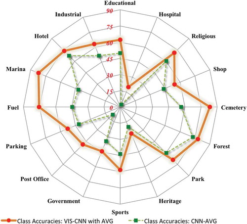
Comparing the baselines with our Siamese Network results, we see that VIS-CNN outperforms the competing methods, both in overall scores (Table 2) and per-class performance (Figure 6). The jump in accuracy is due to the fact that we are training end-to-end the network with ensembles of pictures for each urban-object. This process modifies the earlier layers of the CNN, which can then specialize in the type of structures observed in the landuse dataset. In other words, each picture brings a different point of view of the urban-object, and the representation is learned dynamically by the neural network, which can recombine landuse-tailored representations since the entirety of the VGG network is fine-tuned by the Siamese model. If we compare the two activation aggregators (MAX and AVG) we found that they perform similarly, with the exception of an advantage in AA when using the AVG aggregator.

Figure 6. Accuracies for 16 classes in Ile-de-France. The values are in percentage.

5. Discussion

5.1. Correct predictions

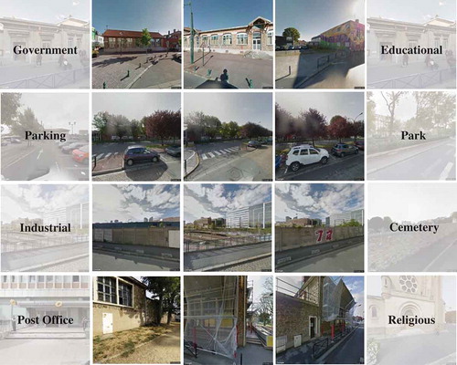
The per-class accuracy scores in Figure 6 shows that the increase in performance is not uniformly distributed among classes: some landuse types (educational institution, religious place, forest, park, fuel station, marina, hotel, industrial area) benefit strongly from the proposed architecture (increase up to 30%). This could be explained by the very discriminative visual cues that these classes carry. For example, in Figure 7, we can see that the architecture of religious places is quite different from any other building in the city. Some examples of correct predictions by VIS-CNN model are illustrated in Figure 7. Pictures for educational institute have visual cues like children, railings, flags while those of category park in the fourth row could be distinguished by the presence of trees, sidewalks, buildings, railings. Similarly, discriminative cues can be found for other classes in Figure 7. From these snapshots, we can appreciate the diversity of GSV pictures used to describe the urban-objects by multiplying the points of view. In addition, the user-generated content also includes complementary data that helps to discriminate some classes. For example, leftmost picture in the first row captures an indoor view of a religious place Figure 8 and it shows seats in rows, candles or statues, while in the second row (leftmost figure) the government building is photographed in the evening Figure 8.

Figure 7. Correct classification by the proposed VIS-CNN model, and examples of GSV pictures involved. Each row represents a single urban-object and some of the GSV pictures used.

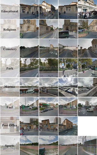
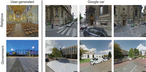
Figure 8. Example of user-generated vs Google car content in the case of (top) religious place and (bottom) governmental building.

5.2. Erroneous predictions

If we can see a general improvement of performance by the proposed model, we also observe that errors of VIS-CNN are not randomly distributed. The radial plots in Figure 9 represent four columns (corresponding to four landuse categories: hospital, heritage, religious, forest) of the confusion matrix obtained by VIS-CNN with the AVG operator (i.e. the types of errors committed for the four classes). In Figure 9, for instance, hospitals are often confused with governmental buildings, while heritage buildings are confused with religious places and government buildings (they all contain sculptures and paintings and tend to have grand exteriors).

Figure 9. Landuse characterization results for four classes. Each radial plot represents one class and the types of error committed. Values in percentages.

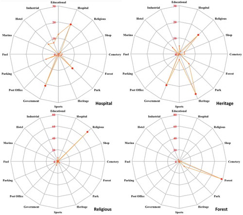
Figure 10. Errors committed by VIS-CNN. The leftmost column corresponds to the true label, while the rightmost column is the wrongly predicted class.

Comparing some of the GSV images (shown in Figure 10) confusion among several classes seems very likely, especially in cases where user-generated content was unavailable. For example, the Google car pictures of the religious place depicted in the first row of Figure 8 are very similar to each other. In contrast, user-generated content gives additional information since it is taken in different lighting conditions, indoor views and closer view-points.

Figure 10 shows examples of erroneous predictions by VIS-CNN, where we can appreciate the difficult task the model is confronted to. For example, the governmental building in the first row shows features similar to schools (low ceiling, wide area in front), while the parking in the second row is surrounded by a park and on some of the pictures show the presence of vegetation primes over the presence of cars. Another interesting example is the industrial area in the third row of Figure 10, which is wrongly predicted as a cemetery. We believe this is due to the long continuous walls that are visible on many pictures. These look like the ones enclosing all the cemeteries in the dataset, which is probably the strongest visual cue learned by the CNN for the cemetery class. The post office in the fourth row is wrongly classified as religious place, possibly because the walls are similar to those of religious places, and the yellow logo of ‘la poste’ is partly occluded.

5.3. Data quality and potential improvements

Although OSM polygons are generally useful to obtain GSV pictures, we found several cases where the OSM polygons did not match with the actual physical boundaries of the urban-objects. We visually verified many GSV pictures and observed that in most cases they captured characteristic features of the corresponding landuse. However, in some cases, the downloaded pictures did not depict the object of interest because of occlusions (for example, due to vehicles on the road, boundary walls, or trees) or poorly digitalized polygon boundaries.

As the boundaries of the urban-objects are digitalized by volunteers, a polygon may partially or completely cover its corresponding urban-object (see Figure 11(a)). Additionally, many urban-object polygons in OSM are not annotated. Therefore, other sources of urban landuse labels could be used to increase our urban-object dataset size.

Figure 11. Issues in our heuristic to download GSV pictures for urban-objects: a) The green lines show the actual physical boundary of urban-object of class ‘government’. This urban-object was assigned a smaller spatial extent by OSM volunteers represented by yellow polygon. Thus the gap between the yellow polygon and the street is more than 12m. As a consequence, the GSV pictures in the second row were missed during the download from Google Street View API. b) There exist building facades which do not face streets but are still at a distance less than 12m from a nearby street. In this case, the GSV pictures downloaded for this urban-object, which is an educational institution, belong to adjacent urban-object, in this case, a veterinary hospital.

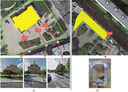
We also found some issues related to our heuristic to download GSV pictures associated with the urban-objects. As mentioned in Section 3, we used a threshold of 12 meters (maximum distance between the urban-object facades and streets in OSM data) to ensure that the pictures that are looking to a particular urban-object facade are taken from a nearby street. This heuristic alone is not a guarantee of extracting only relevant pictures. Sometimes using this threshold value leads to GSV pictures that are associated with another nearby urban-object falling in the distance range (Figure 11(b)). In other cases, GSV pictures of an urban-object are missing because the nearest street was at a distance greater than 12 meters. The latter problem happens also because OSM polygons sometimes cover a lesser spatial extent than the actual physical boundaries of the urban-objects (see Figure 11(a)).

An important potential improvement of the urban-object dataset is the availability of user-generated content: for many urban-objects, indoor views are missing in GSV, while we have observed that such pictures carry very distinctive information. In general, indoor and outdoor scenes depict different objects and visual cues. Taking church as an example, the corresponding indoor pictures contain objects like chandeliers, lamps, candles, statues, and chairs, while outdoor pictures depict visual attributes like large arches, stone walls and rose glasses. One possible solution would be to resort to pictures from alternative social media platforms. Although geo-referenced pictures available on social media require a lot of pre-processing, they could possibly be utilized to improve the training of the classifier. For example, pictures from within a shop or a restaurant would help discern the two classes which look similar from outside. Most pictures from GSV are during the daytime. Thus, adding pictures from other times of the day available on social media could probably make the classifier more robust to the lighting conditions. In addition to including more discriminative pictures in the dataset, we can also increase the number of labeled urban-objects by including annotations provided by Google places API, as in (Zhu et al. 2018).

6. Conclusion

This paper presents a new methodology for landuse characterization based on deep learning and open geospatial data. We demonstrated the usefulness of freely available data (GSV pictures and OSM shapes) to the task. Driven by intuition that landuse cannot be reduced to a single view of the territory, we proposed a deep learning solution capable of taking into account multiple image snapshots of an urban-object. To this end, we designed a CNN that takes a variable number of pictures as inputs. This specific characteristic makes the model versatile and able to predict landuse in very diverse situations, both in terms of content and images available. Our proposed model combines the various viewpoints to understand the context of the classes. Through a case study in Île-de-France, we showed that the accuracy of our proposed model has significant improvement over the competing methods.

Thanks to the fact that the convolutional layers are shared between the different branches of the network, the model stays light in terms of memory, is relatively fast to train and is robust to the variability of pictures pertaining to an urban-object. Such characteristics are desirable for a solution aiming at automating landuse characterization maps and their updates. In the future, our model could complement field-based methods which are traditionally time-consuming, expensive, and human resource intensive.

As a future work, this method should be tested in different urban areas, with a double objective: on the one hand, to stress-test its effectiveness in different architectural, climatic and cultural contexts, and on the other hand to study the potential of transferability of the learned model without landuse labels from the new city under study. We intend to improve the performances of VIS-CNN by using labels provided by Google Places API and integrating other sources of image data, including social media. Another promising research avenue would be to enrich the current model with additional informative visual cues such as detected outdoors marking signs (which could be helpful in recognizing text and keywords) or the use of overhead images.

Acknowledgments

The authors would like to thank Google and OSM for the access to pictures and objects’ footprints, respectively, through their APIs. This work has been supported by the Swiss National Science Foundation (SS, SL, DT, grant PZ00P2-136827, http://p3.snf.ch/project-136827) and by the São Paulo Research Foundation FAPESP (JEVM, grant 2017/10086-0).

Disclosure statement

No potential conflict of interest was reported by the authors.

Additional information

Funding

This work was supported by the Fundação de Amparo à Pesquisa do Estado de São Paulo [2017/10086-0];Schweizerischer Nationalfonds zur Förderung der Wissenschaftlichen Forschung [PZ00P2-136827]

Notes

1. http://www.un.org/en/development/desa/population/publications/pdf/urbanization/the_worlds_cities_in_2016_data_booklet.pdf.

2. We define an urban-object as a spatial construct in an urban space with a clear physical boundary of its own, which could be a closed construct (like shop, office), semi-open construct (like stadium), or an open space (natural like forest or man-made, like park).

3. For the most recent coverage, see https://www.google.com/streetview/understand/.

4. https://developers.google.com/maps/documentation/streetview/.

5. More information about privacy and blurring: https://www.google.com/streetview/privacy/; Usage terms and conditions: https://developers.google.com/maps/terms.

6. https://www.openstreetmap.org/.

7. http://pytorch.org/.

Appendix: per class landuse prediction plots

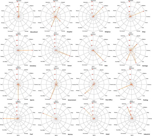
Figure A1 represents each column of the confusion matrix obtained by VIS-CNN with the AVG operator, or, in other words, the types of errors committed for each class.

Figure A1. Per-class landuse characterization results. Each radial plot represents one class and the types of error committed. Values in percentages.

References

- Bromley, J., et al., 1994. Signature verification using a “Siamese” time delay neural network. In: Proceedings of the 6th International Conference on Neural Information Processing Systems (NIPS'93), Denver, Colorado, 737-744.
- Chen, Y.H., et al., 2017. No more discrimination: cross city adaptation of road scene segmenters [online]. In: IEEE International Conference on Computer Vision (ICCV), 2011–2020, Venice, Italy. Available from: https://ieeexplore.ieee.org/document/8237482
- Doersch, C., et al. 2012. What makes paris look like Paris? ACM Transactions on Graphics, 31 (4), 101:1–101: 9. doi:10.1145/2185520.2185597
- Gebru, T., et al., 2017. Using deep learning and google street view to estimate the demo- graphic makeup of neighborhoods across the United States. Proceedings of the National Academy of Sciences.
- Goodfellow, I., Bengio, Y., and Courville, A., 2016. Deep Learning [online]. Cambridge, MA: MIT Press. Available from: https://scholar.googleusercontent.com/scholar.bib?q=info:MHq4MMenr-gJ:scholar.google.com/&output=citation&scisig=AAGBfm0AAAAAW-BR28x8tJC3_K616H6eijqFQDTM_U8m&scisf=4&ct=citation&cd=-1&hl=en
- Homer, C., et al., 2015. Completion of the 2011 National Land Cover database for the conter- minous United States–representing a decade of land cover change information. Photogram- Metric Engineering & Remote Sensing, 81 (5), 345–354.
- Krizhevsky, A., Sutskever, I., and Hinton, G.E., 2012. Imagenet classification with deep convo- lutional neural networks [online]. Advances in neural information processing systems, Lake Tahoe, Nevada, 1097–1105. Available from: https://dl.acm.org/citation.cfm?id=2999257
- Laptev, D., et al., 2016. TI-POOLING: transformation-invariant pooling for feature learning in convolutional neural networks [online]. In: Proceedings of the IEEE Conference on Computer Visionand Pattern Recognition (CVPR), Las Vegas, 289–297. Available from: https://www.cv-foundation.org/openaccess/content_cvpr_2016/html/Laptev_TI-Pooling_Transformation-Invariant_Pooling_CVPR_2016_paper.html
- Lefevre, S., et al. 2017. Towards seamless multi-view scene analysis from satellite to street- level. Proceedings of the IEEE, 105 (10), 1884–1899. doi:10.1109/JPROC.2017.2684300
- Movshovitz-Attias, Y., et al., 2015. Ontological supervision for fine grained classification of street view storefronts [online]. In: Proceedings of the IEEE Conference on Computer Vision and Pattern Recognition (CVPR), Boston, MA, 1693–1702. Available from: https://ieeexplore.ieee.org/document/7298778
- Naik, N., et al. 2017. Computer vision uncovers predictors of physical urban change. Proceed- Ings of the National Academy of Sciences, 114 (29), 7571–7576. doi:10.1073/pnas.1619003114
- Nair, V. and Hinton, G.E., 2010. Rectified linear units improve restricted boltzmann machines [online]. In: Proceedings of the 27th international conference on machine learning (ICML), Haifa, Israel, 807–814. Available from: https://dl.acm.org/citation.cfm?id=3104425
- Pacifici, F., Chini, M., and Emery, W.J., 2009. A neural network approach using multi-scale textural metrics from very high-resolution panchromatic imagery for urban land-use classi-fication. Remote Sensing of Environment, 113 (6), 1276–1292. doi:10.1016/j.rse.2009.02.014
- Postadjiana, T., et al., 2017. Investigating the potential of deep neural networks for large-scale classification of very high resolution satellite images [online]. ISPRS annals of the photogrammetry. Remote Sensing and Spatial Information Sciences, IV-1/W1, 4. Available from: https://www.isprs-ann-photogramm-remote-sens-spatial-inf-sci.net/IV-1-W1/183/2017/
- Produit, T., et al., 2014a. Do geographic features impact pictures location shared on the web? modeling photographic suitability in the Swiss Alps [online]. In: Environnmental Multimedia Retrieval co-located with ACM International Conference on Multimedia Retrieval, Glasgow, UK, 22–29. Available from: https://www.researchgate.net/publication/288711832_Do_geographic_features_impact_pictures_location_shared_on_the_Web_Modeling_photographic_suitability_in_the_Swiss_Alps
- Produit, T., et al., 2014b. Pose estimation of web-shared landscape pictures. ISPRS annals of the photogrammetry. Remote Sensing and Spatial Information Sciences, 2 (3), 127.
- Simonyan, K. and Zisserman, A., 2014. Very deep convolutional networks for large-scale image recognition. CoRR, abs/1409.1556.
- Srivastava, S., et al., 2018. Land-use characterisation using google street view pictures and openstreetmap [online]. In: Proceedings of the Association of Geographic Information Laboratories in Europe Conference (AGILE), Lund, Sweden. Available from: https://agile-online.org/conference_paper/cds/agile_2018/shortpapers/65%20Paper_ID_65_AGILE2018_Landuse_Characterisation.pdf
- Tracewski, L., Bastin, L., and Fonte, C.C., 2017. Repurposing a deep learning network to filter and classify volunteered photographs for land cover and land use characterization. Geo-Spatial Information Science, 20 (3), 252–268. doi:10.1080/10095020.2017.1373955
- Tuia, D., Flamary, R., and Courty, N., 2015. Multiclass feature learning for hyperspectral image classification: sparse and hierarchical solutions. ISPRS Journal of Photogrammetry and Remote Sensing, 105, 272–285. doi:10.1016/j.isprsjprs.2015.01.006
- Wegner, J.D., et al., 2016. Cataloging public objects using aerial and street-level images-urban trees. In: Proceedings of the IEEE Conference on Computer Vision and Pattern Recognition (CVPR), Las Vegas, 6014–6023.
- Workman, S., et al., 2017. A unified model for near and remote sensing. In: Proceedings of the IEEE International Conference on Computer Vision (ICCV), Venice, Italy.
- Zeiler, M.D. and Fergus, R., 2014. Visualizing and understanding convolutional networks. In: Proceedings of the European Conference on Computer Vision (ECCV). Zurich: Springer, 818–833.
- Zhou, B., et al., 2014. Recognizing city identity via attribute analysis of geo-tagged images. In: European conference on computer vision (ECCV). Zurich: Springer, 519–534.
- Zhu, X., et al. 2017. Deep learning in remote sensing: a comprehensive review and list of resources. IEEE Geoscience and Remote Sensing Magazine, 5 (4), 8–36. doi:10.1109/MGRS.2017.2762307
- Zhu, Y., Deng, X., and Newsam, S., 2018. Fine-grained Land Use classification at the city scale using ground-level images. arXiv:1802.02668 [cs]. ArXiv: 1802.02668.