Embedding road networks and travel time into distance metrics for urban modelling

ABSTRACT

Urban environments are restricted by various physical, regulatory and customary barriers such as buildings, one-way systems and pedestrian crossings. These features create challenges for predictive modelling in urban space, as most proximity-based models rely on Euclidean (straight line) distance metrics which, given restrictions within the urban landscape, do not fully capture spatial urban processes. Here, we argue that road distance and travel time provide effective alternatives, and we develop a new low-dimensional Euclidean distance metric based on these distances using an isomap approach. The purpose of this is to produce a valid covariance matrix for Kriging. Our primary methodological contribution is the derivation of two symmetric dissimilarity matrices ($B^{+}$ and $B^{2+}$), with which it is possible to compute low-dimensional Euclidean metrics for the production of a positive definite covariance matrix with commonly utilised kernels. This new method is implemented into a Kriging predictor to estimate house prices on 3,669 properties in Coventry, UK. We find that a  metric estimating a combination of road distance and travel time, in both ${\mathbb{R}}^2$ and ${\mathbb{R}}^3$, produces a superior house price predictor compared with alternative state-of-the-art methods, that is, a standard Euclidean metric in ${\mathbb{R}}^{\mathbb{N}}$ and a non-restricted road distance metric in ${\mathbb{R}}^2$ and ${\mathbb{R}}^3$. F

KEYWORDS:

• Geostatistics
• data mining
• Kriging
• non-Euclidean
• real-estate
• urban analytics
• isometric embedding
• multidimensional scaling

1. Introduction

By 2030, it is expected that 5 billion people will live in urban areas, 662 cities will have at least 1 million residents and there will be a total urban spread of 1.2 million km² (Biello 2012, Seto et al. 2012, Nations 2016). Hence, cities will continue to accommodate over 50% of the world’s population.

In the United Kingdom, over 82% of citizens live in its 64 cities, a figure which has grown by more than 13% in the past 30 years (Champion 2014). Many UK cities suffer from legacy infrastructure – the City of London, for example, relies on sewage infrastructure originally built in the 1860s – which impacts on their ability to support projected growth. Such challenges are well documented: Housing supply is not matching demand (Henretty 2018), commuting times are increasing (Gayle 2017) and there are shortages in services for the most vulnerable citizens (Stewart et al. 2003). Issues of urban growth and sustainability motivate the development of mathematical tools and models for explanatory and predictive analysis (Townsend 2015).

Urban models provide insight into the relationship between some chosen target value, house prices for example, and other potentially related variables, such as topography (Kok et al. 2011), building footprints (Pace et al. 1998) and crime (Thaler 1978). Space (Crosby et al. 2016) and time (Huang et al. 2010) consistently feature in most urban models, for example in house price prediction (Crosby et al. 2018), traffic flow prediction (Zou et al. 2012) and in the analysis of green space and its impact on well-being (Houlden et al. 2017). A typical approach to understanding spatial characteristics in this way is through geostatistical proximity-based modelling. An example of this approach is Kriging (defined in Section 4), which assumes random variables to be spatially dependent and non-stationary over space.

A common assumption in geostatistical models (including Kriging) is that proximity is based on Euclidean distance; this is in spite of the fact that dispersion in a city landscape is unlikely to exhibit such properties.

Traditionally, research in real-estate price modelling has considered distance to a specific location (e.g. workplace) and/or comparable prices of other sub-markets within close proximity. A more sophisticated approach to this is to include physical barriers such as buildings, road layout and non-accessible open space to the models, as distance, in practice, is clearly governed by such obstacles. This is evident in recent work on road distance-based Kriging, which has been shown to be highly effective for urban house price prediction (Crosby et al. 2018).

Our paper presents a natural extension to this earlier work by including travel time. In so doing, it integrates a number of otherwise difficult-to-capture variables such as traffic flow, road layout, junction priority and congestion caused by on-road parking. Our primary purpose is to show the effect that road distance and travel time have on predictive modelling; note that we do not prescribe reasons for these effects (i.e. we will not be considering any covariates).

Our methodological advances are motivated by our work in urban house price prediction; that is, we attempt to model unexplained variation through proximity between observations, to underpin and improve on hedonic pricing models already available in academia and in industry.

An essential prerequisite to geostatistical models is the production of a variogram and covariance function. Covariance and variogram functions must remain valid – positive definite (PD) and conditionally negative definite (CND), respectively (Curriero 2005, 2006) (see Section 4.1 for formal definition).

Given the extensive research based on Euclidean pairwise distance (straight lines), there is no guarantee that any non-Euclidean distance matrix (PD or otherwise) will produce valid covariance or variogram functions. For this reason, pairwise road distance and travel time matrices are unlikely to be valid. Hence, the purpose of this research is to propose an isometric embedding approach with which we can approximate road distance and travel time in a lower dimensional Euclidean space, to allow physical properties of cities to be represented in spatial prediction whilst still producing mathematically valid approximations.

In order to illustrate the benefits of these new distance metrics, a so-called real-estate automated valuation model (AVM) for residential properties is developed for the city of Coventry in the United Kingdom. This AVM is used to provide mathematically modelled individual market values for 3669 properties. The case study in Section 5 shows that a combination of road distance and travel time produces a superior Kriging predictor compared with a Euclidean approach for all assessed validation metrics.

1.1. Contributions

The contributions of this research are as follows:

• First, methodological contributions are made via the derivation of two symmetric dissimilarity matrices ($B^{+}$ and $B^{2+}$), with which it is possible to compute low-dimensional Euclidean metrics for the production of a PD covariance matrix with commonly utilised kernels and non-valid, non-Euclidean, input spaces.

• Second, we demonstrate the application of this new geostatistical approach to the calculation of (1) approximate restricted road distance, (2) approximate travel time and (3) combined road distance and travel time matrices, in each case within an embedded lower dimensional Euclidean space.

• Third, we compare a number of the most popularly employed cross-validation techniques to assess the ability of each to estimate how well our model generalises to unseen data.

1.2. Sections

The remainder of this paper is organised as follows: background research is detailed in Section 2; Section 3 motivates the need for this research through two practical examples; new methodological contributions are described in Section 4 and applications of these methods, to urban house price prediction, can be found in Section 5. The paper concludes in Section 6 in which we also document avenues for future research.

2. Related literature and key concepts

2.1. Constructing optimal urban Kriging predictors

Kriging is a geostatistical spatial predictor which accounts for spatial covariance. The method utilises observation distances to understand the spatial structure of a dataset and hence determine its own interpolation parameters (Cressie 2015). Kriging is used extensively for interpolation by ecologists (Little et al. 1997), geographers Changling (1987) application and geo-scientists (Hudson and Wackernagel 1994). The first stage of Kriging models the degree to which distance between observations is correlated. The experimental variogram does this by calculating an average difference between observations (termed the lag). If the experimental variogram is able to observe spatial patterns accurately, then Kriging applies the modelling coefficients to determine interpolation parameters (Matheron 1963). Parameter optimisation, kernel selection and lag sizes are the primary strategies used in optimising experimental variogram and Kriging algorithms (Cressie 1985, Garcıa-Soidán et al. 2004, Yu et al. 2007).

Kriging is commonly used in urban science and examples of its application include traffic flow prediction (Zou et al. 2012), and travel time (Miura 2010) and trip planning (Liebig et al. 2014). The use of Kriging for urban real-estate pricing is motivated by Dubin (1988), Basu and Thibodeau (1998) and Crosby et al. (2016) who together note that space and time are highly influential in house price prediction. Each of these approaches however uses Euclidean distance only.

A small number of non-Euclidean distance-based approaches have been employed to Kriging, including those based on Minkowski (including Manhattan) (Ganio et al. 2005, Theodoridou et al. 2015, Crosby et al. 2018), geodetic (Banerjee 2005) and water-based (shortest path over water) (Murphy et al. 2014) distances. Each offers its own benefits; however, it is difficult to assess whether each produces valid experimental variograms without access to the initial data; we show in Section 3 that relying on the fact that input distances are PD metrics is no guarantee of valid variograms.

In a similar manner to this research, Crosby et al. (2018) utilises Open Street Map (OSM) data to estimate restricted road distance and travel time between pairwise points. Crosby et al. (2018) uses a Minkowski $P$ value of 1.6, which demonstrates the highest correlation to road distance, travel time and a linear combination of both, with the OSM data. Their work also discovered that the same $P$ value returned positive results when applied to the domain of house price prediction. We directly compare the results of Crosby et al. (2018) with our new approach, see Section 5. Figure 1 provides a simple comparison of Minkowski distance (P = 1.6), a Euclidean distance, a Manhattan distance and regular road distance.

Research which bears similarity to our own can be found in Lu et al. (2014), who use geographically weighted regression (GWR) and a non-Euclidean distance metric for predicting London house prices. Their research also utilises road distance and travel time, however is limited to network shape and speed limit; our measures include a wealth of other data provided by OSM, see Table 5.

Table 1. A list of all datasets, sources and descriptions used in our case study.

Dataset	Source	Description
House prices	Land Registry	A list of $n$ actual sold prices for each house $i$ in Coventry
House locations	Ordnance Survey	A list of n long/lat points for location $i$
Restricted road	OSRM	A pairwise distance matrix containing an average daily restricted road distance
Travel time	OSRM	A pairwise distance matrix containing an average daily travel time
Road network	Ordnance Survey	A node-edge diagram of Coventry City with no legal or restrictive barriers, e.g. this network does not take into account one-way systems

Table 2. Example restrictions to road networks from OSM labels.

Restriction type	Description
Barrier	(Rising) bollard, cattle grid, toll booth etc.
Restriction	Motor vehicle, vehicle, permissive, designated, destination, private, agricultural, forestry, emergency, parking aisle etc.
Speed profile	Motorway, trunk, primary, secondary, tertiary etc.
Surface speeds	Concrete, paved, cement, compacted, paving stones, metal, grass, gravel, unpaved, cobblestone, stone, sand, mud etc.
Max speed	Urban, rural, trunk, motorway, single/dual carriageway
U-turns and traffic signal	Time (s)
One way	Boolean (y/n)
Route speed	Ferries, piers, movable bridges

Table 3. The $r^2$ values for each distance metric compared with actual road distance and travel time matrices.

Experiment	Distance Metric	Actual road Distance ($r^2$)	Actual travel Time ($r^2$)
1	$D_{Euc}$	0.377	0.359
2	$D_{Mink}$	0.379	0.359
3	$D_{FW}^{\prime }$	0.374	0.365
4	$D_{RD}^{\prime }$	0.621	0.592
5	$D_{TT}^{\prime }$	0.606	0.614
6	$D_{RDTT}^{\prime }$	0.446	0.419

Table 4. Selected hyperparameters for all experiments (1)–(6) (Exp. 1–6) with dead-zone 10-fold cross-validation.

	Euclidean	Minkowski	PD road	Road	Travel	Combined
	Distance (Exp. 1)	Distance (Exp. 2)	HaixongDistanceMatric (Exp. 3)	Distance (Exp. 4)	Time (Exp. 5)	Matrices (Exp. 6)
$Nugget$	0.03	0.003	0.0035	0.018	0.0015	0.008
$Sill$	0.07	0.03	0.02	0.03	0.05	0.05
$Range$	20,000	20,000	15,000	15,000	30	30,000
Kernel	Matern	Matern	Matern	Gaussian	Spherical	Spherical

Table 5. Results from four validation techniques: 10-fold cross-validation, spatially stratified 10-fold cross-validation, chequerboard holdout and spatial dead-zone 10-fold cross-validation.

Result tables
	Previously implemented techniques for comparison			Newly defined techniques
	P = 2 (Euclidean) (Exp. 1)	P = 1.6 (Minkowski) (Exp. 2)	No road restriction (Exp. 3)	Road distance (Exp. 4)	Travel time (Exp. 5)	Combined matrices (Exp. 6)	Optimistic
			10-Fold validation
$r^2$	0.81$\pm$0.3	0.8$\pm$0.18	0.79$\pm$0.03	0.82$\pm$0.06	0.81$\pm$0.06	0.82$\pm$0.04
$RMSE$	55,177$\pm$13,034	74,786$\pm$29,266	65,088$\pm$15,481	57,322$\pm$18,958	59,294$\pm$12,830	78,158$\pm$21,742
$MAPE$	17.9$\pm$1.1%	24.5$\pm$6.9%	20.7$\pm$1.74%	21.5$\pm$1.6%	18.1$\pm$1.9%	25.2$\pm$1.7%
			Spatial 10-fold stratified validation
$r^2$	0.42$\pm$0.21	0.44$\pm$0.26	0.47$\pm$0.34	0.46$\pm$0.24	0.46$\pm$0.17	0.44$\pm$0.25
$RMSE$	87,081.2$\pm$68,889	87,539$\pm$78,597	78,744$\pm$36,831	71,601$\pm$62,217	75,905$\pm$68,296	77,839$\pm$68,127
$MAPE$	32.3$\pm$21.2%	30.4$\pm$22.5%	26.8$\pm$11.5%	25.7$\pm$10.02	26.5$\pm$12.3	26.6$\pm$13.6%
			Chequerboard stratified validation
$r^2$	0.44	0.46	0.5	0.51	0.51	0.52
$RMSE$	82,972	81,940	76,850	72,770	75,226	74,816
$MAPE$	26.7%	26.2%	24.9%	23.8%	26.1%	25.3%
			Dead zone 10-fold cross-validation 20 m
$r^2$	0.23$\pm$0.13	0.29$\pm$0.32	0.53$\pm$0.16	0.5$\pm$0.09	0.4$\pm$0.15	0.56$\pm$0.05
$RMSE$	97,079$\pm$18,491	100,201$\pm$39,526	85,770$\pm$11,052	87,730$\pm$21,736	97,892$\pm$22,792	85,413$\pm$9138	Pessimistic
$MAPE$	31.2$\pm$3.4%	34.7$\pm$4.6%	28.3$\pm$2.5	26.5$\pm$3.02	31.3$\pm$3.9	27.2$\pm$2.9

Approaches based on GWR have advantages, in particular because there is no requirement for the matrix to be Euclidean [the matrix $w_i$ of weights is diagonal; hence, there is no need to check for positive definiteness, which is not the case with the covariance matrix used in Kriging (Curriero 2006)]. However, it is noted in Crosby et al. (2018) that Kriging typically outperforms GWR in spatial pricing models; this is especially true when implemented locally, which is the case in Ordinary Kriging which assumes intrinsic stationarity (i.e. a moving mean but a stationary variance between any two points).

2.2. Overcoming non-metric input spaces

For the most part, geostatistics relies on the assumption that each set of distances lie in a metric space $(\mathbf{M},d)$, where $\mathbf{M}$ is a set and $d$ is a metric on $\mathbf{M}$; for example, $d$ might be a function:

(1) $d:MXM\to {\mathbb{R}}^{+}.$(1)

${\mathbb{R}}^{+}\in \mathbb{M}$ is a set of non-negative real numbers whose values satisfy the properties P1–P4:

$d_{i,j}>0$ (P1: Non negativity)

$d_{i,j}=0\Leftarrow x_i=x_j$ (P2: Identity of indiscernibles)

$d_{i,j}=d_{j,i}(\mathrm{P}3:\mathrm{S}\mathrm{y}\mathrm{m}\mathrm{m}\mathrm{e}\mathrm{t}\mathrm{r}\mathrm{y})$

$d_{i,j}<d_{i,k}+d_{k,j}$ (P4: Triangle inequality).

There are three known methods which ensure that a distance matrix is valid (i.e. it produces a PD covariance matrix): the first uses isometric embedding to ensure a Euclidean input; the second is the use of kernel convolution so that the kernel fits any matrix; the third is to select a matrix which produces a valid covariance matrix. Previous research has assumed that the distance matrix does not have to satisfy P1–P4 per se, but that it must ensure a PD covariance matrix. We do not subscribe to this view, as the example in Section 3 highlights.

With regard to the three methods that ensure matrix validity: Isometric embedding provides a dimensionality reduction technique with which it is possible to build a low dimensional Euclidean approximation of non-Euclidean inputs for variogram modelling. Using simulated data with isotropic spatial dependence, Curriero (2006) builds four omnidirectional experimental variograms, each representing an $\alpha$ norm, for $\alpha$ = 1, …, 4 ($\alpha$ = 2 is Euclidean). When these data are applied with Kriging, the newly defined ‘stream’ distances outperform Euclidean distances in all cases; this is therefore our method of choice.

We note that other research proposes similar approaches to approximate road distance metrics, see Tenenbaum et al. (2000) and Zou et al. (2012). In Zou et al. (2012), the Floyd Warshall (FW) algorithm is applied to a road network to estimate the actual road distance between pairwise locations. We note however that FW only selects the shortest distance, irrespective of restrictions such as transport patterns and one-way systems.

The use of kernel convolutions, which can be used to express moving averages, assumes that correlated data can be expressed as linear combinations of uncorrelated data. This method has been successfully applied by Crawford and Young (2008); however, we note that this method can be difficult to implement on problems with large datasets and is hence not considered further in this work.

Finally, the selection or creation of a valid covariance function can be undertaken. For example, Curriero (2006) noted that a set of Manhattan distances produced non-valid variograms with Gaussian, Matern and spherical kernels but were valid for an exponential kernel. We are aware that this approach has several restrictions and is also time consuming to compute, and so for this reason, isometric embedding remains our method of choice.

3. Motivation

The contributions of this work are based on the following assertion: The only way to guarantee that a covariance matrix and variogram function are valid in this context is to ensure that a Euclidean distance metric is input for their calculation.

The only way to ensure that a variogram is valid is to input a Euclidean distance function. This implies that even PD distance functions cannot always produce a valid variogram, a concept which has potential to invalidate much previous research.

3.1. Non-PD inputs

Non-PD matrices produce non-PD kernels (covariance functions) which is usually as a consequence of the $L_2$ norm; note that Section 3.2 provides other examples where this is the case. Matrices 1 and 2 show a set of possible pairwise distances. These matrices are not symmetric, much like a road network containing one-way systems, and hence, they are not PD. To test whether each matrix always produces a valid variogram, we select a Gaussian covariance function ($C(h)={\sigma }^2{e}^{{(-h/a)}^2}$) with ${\sigma }^2$ = 0.5, 0.08 and a = 450, 1.5. The output vectors from this calculation are shown in Vectors 1 and 2.

Matrix 1. Road distance (m).Matrix 2. Travel time (min).

$\left[\begin{array}{cccccccc}\hspace{0.17em}& \mathbf{1}& \mathbf{2}& \mathbf{3}& \mathbf{4}& \mathbf{5}& \mathbf{6}& \mathbf{7}\\ \mathbf{1}& 0& 266.5& 459.4& 738.1& 602.5& 614.3& 640.6\\ \mathbf{2}& 266.5& 0& 321.6& 600.3& 464.8& 476.5& 502.8\\ \mathbf{3}& 459.4& 321.6& 0& 278.7& 143.1& 154.9& 181.2\\ \mathbf{4}& 738.1& 600.3& 278.7& 0& 346.6& 358.4& 342.4\\ \mathbf{5}& 602.5& 464.8& 143.1& 346.6& 0& 358.4& 342.4\\ \mathbf{6}& 614.3& 476.5& 154.9& 358.4& 222.8& 0& 133.8\\ \mathbf{7}& 640.6& 502.8& 181.2& 384.7& 249.1& 133.8& 0\end{array}\right]\left[\begin{array}{cccccccc}\hspace{0.17em}& \mathbf{1}& \mathbf{2}& \mathbf{3}& \mathbf{4}& \mathbf{5}& \mathbf{6}& \mathbf{7}\\ \mathbf{1}& 0& 0.81& 1.188& 1.186& 1.71& 1.628& 1.75\\ \mathbf{2}& 0.702& 0& 0.855& 1.523& 1.38& 1.29& 1.42\\ \mathbf{3}& 1.133& 0.8& 0& 0.67& 0.522& 0.44& 0.56\\ \mathbf{4}& 1.8& 1.47& 0.67& 0& 0.96& 0.982& 1.05\\ \mathbf{5}& 1.55& 1.212& 0.412& 0.956& 0& 0.603& 0.723\\ \mathbf{6}& 1.681& 1.348& 0.548& 0.98& 0.72& 0& 0.44\\ \mathbf{7}& 1.7& 1.36& 0.56& 0.99& 0.72& 0.44& 0\end{array}\right]$

Vector 1. Road distance.Vector 2. Travel time.

$\left[\begin{array}{c}2.09991\\ 0.74078\\ 0.27006\\ 0.22365\\ 0.13790\\ 0.04218\\ -0.0145\end{array}\right]\mathrm{a}\mathrm{n}\mathrm{d}\left[\begin{array}{c}0.38814\\ 0.098924\\ 0.03598\\ 0.018321\\ 0.010134+0.00194i\\ 0.010134-0.00194i\\ -0.014469\end{array}\right]$

In view of the negative roots in Vectors 1 and 2, it is clear that both covariance functions are not conditionally PD (${\sum }_{i=1}^n{\sum }_{j=1}^n{\alpha }_i{\alpha }_{j}C(h)\ge 0$) and hence road distance and travel time are not valid for variogram modelling.

3.2. PD inputs

Additionally, non-Euclidean PD matrices may also produce non-PD kernels, a fact that previous research has been known to overlook. Matrix 3 below represents the same roads as in Matrix 1 and 2, but this time, the road distance is not restricted (much like the work by Zou et al. 2012); that is to say, one-way systems are not considered and hence are completely PD. The same covariance function and hyperparameters are used.

Matrix 3. Road distance (m).

$\left[\begin{array}{cccccccc}\hspace{0.17em}& \mathbf{1}& \mathbf{2}& \mathbf{3}& \mathbf{4}& \mathbf{5}& \mathbf{6}& \mathbf{7}\\ \mathbf{1}& 0& 266.5& 459.4& 738.1& 602.5& 614.3& 640.6\\ \mathbf{2}& 266.5& 0& 321.6& 600.3& 464.8& 476.5& 502.8\\ \mathbf{3}& 459.4& 321.6& 0& 278.7& 143.1& 154.9& 181.2\\ \mathbf{4}& 738.1& 600.3& 278.7& 0& 346.6& 358.4& 384.7\\ \mathbf{5}& 602.5& 464.8& 143.1& 346.6& 0& 222.8& 249.1\\ \mathbf{6}& 614.3& 476.5& 154.9& 358.4& 222.8& 0& 133.8\\ \mathbf{7}& 640.6& 502.8& 181.2& 384.7& 249.1& 133.8& 0\end{array}\right]$

Vector 3. PD road distances.

$\left[\begin{array}{c}2.1346\\ 0.74503\\ 0.30465\\ 0.153779\\ 0.12919\\ 0.039961\\ -0.0072856\end{array}\right]$

Vector 3 shows that the output eigenvector still contains negative roots, which itself means that the covariance function is not conditionally PD, despite the input matrix being PD. This motivates our new approach for estimating non-Euclidean, non-PD distance matrices in a Euclidean space in order to produce valid covariance and variogram functions.

4. Method

We describe how current state-of-the-art approaches estimate city-based proximity (i.e. non-Euclidean distance metrics) and compare these approaches to our new method. We show how our proposed approach, isometric embedding with two symmetric dissimilarity matrices ($B^{+}$ and $B^{2+}$), produces a PD covariance matrix. As a result of this, we then show application of this new technique to the establishment of an urban real-estate price predictor.

4.1. Distance matrix calculation

To undertake geostatistical modelling, a pairwise distance metric is required. This pairwise distance metric is populated with distances $d_{i,j}$ from a list of locations {$x_i,i=1,\dots ,n$} in Euclidean space ${\mathbb{R}}^n$. The matrix provides the basis for a valid metric if all $d_{i,j}$ satisfy P1–P4, see Section 2.2.

As we have previously shown, road distance and travel time are not natural metrics. Given this, we compare four methods for calculating conforming geostatistical distance metrics from these inputs: (1) A Euclidean distance (see Section 4.1.1), (2) a Minkowski approximation of restricted road distance and travel time (see Section 4.1.2), (3) an isomap estimate of road distance (see Section 4.1.3) and (4) a newly formulated improved isometric embedding approach to estimating restricted road distance and travel time (see Section 4.1.3).

4.1.1. Euclidean distance

Unless otherwise stated, it is typical to assume a Euclidean function when referring to distance. Assuming two sites as vectors s = $(s_1,\dots ,s_d)$ and u = $(u_1,\dots ,u_d)$, in Euclidean space ${\mathbb{R}}^d$, then the Euclidean distance is

(2) $\left|\left|\mathbf{s}-\mathbf{u}\right|\right|={\left\{\sum _{i=1}^d(s_i-u_i{)}^2\right\}}^{\frac{1}{2}},$(2)

where $d$ is the number of dimensions (or attributes) and $s_i$ and $u_i$ are the attributes.

4.1.2. Minkowski distance

Assuming the same notation as above, the Minkowski distance is

(3) $\left|\left|\mathbf{s}-\mathbf{u}\right|\right|={\left\{\sum _{i=1}^d||(s_i-u_i{)}^P\right\}}^{\frac{1}{P}},$(3)

where $P$ is an user-defined parameter. Manhattan and Euclidean distances are special cases of Minkowski, with P = {1,2}, respectively. Crosby et al. (2018) show that Minkowski distances with $P\ne$ {1,2} can better estimate road distance and travel time compared with Manhattan or Euclidean distances.

4.1.3. Isometric embedding and isomap

Isometric embedding provides the spatial transformation of a new metric space ${\zeta }^{\prime }$=$(s^{\prime },d^{\prime })$ from $\zeta =(s,d)$, with point set $s=(s_1,s_2,\dots ,s_n)$, distance function D of $\zeta$ and distance function D′ of ${\zeta }^{\prime }$. All associated $s$ and $d_{ij}$ values are intrinsic. If D $\simeq$ D′, then the transformation still preserves topological adjacency among points in the original space $\zeta$. Dimensionality reduction is a good means of achieving isometric embedding; multidimensional scaling (MDS) is the most popular such scheme.

Isomap, in addition to isometric embedding, attempts to detect the intrinsic characteristics of non-linear data, in which $\zeta$ may be a non-metric space. For example, isometric embedding assumes a Euclidean distance, whereas isomap supports other spatial features such as non-restricted approximate road (Zou et al. 2012) and geodesic (Banerjee 2005) distances on a set of discrete points (Tenenbaum et al. 2000). Figure 2 provides an example of a road distance layout (left) transformed into a low-dimensional Euclidean space (right) using isomap.

As stated, MDS is a dimensionality reduction technique used to achieve isometric embedding or isomap. Given an input metric D (which is e.g. Euclidean) in n-dimensional metric space $\zeta$, the first stage of MDS is to calculate the dissimilarity matrix $B$

(4) $B=\frac{1}{2}\left\{a_{ij}-a_i.-a_j.+a..\right\}$(4)

where $a_i.$ is the average of all $a_{ij}$ across $j$. Formally, each element $B_{ij}$ in matrix $B$ is calculated by

(5) $B_{ij}^{\ast }=\frac{1}{2}\left(-d_{ij}^2+\frac{1}{n}\sum _{l=1}^n{d}_{il}^2+\frac{1}{n}\sum _{l=1}^n{d}_{lj}^2-\frac{1}{n^2}\sum _{l=1}^n\sum _{m=1}^n{d}_{lm}^2\right)$(5)

where B is a new set of isometric distances which mimics a kernel where B is doubly centred. Although B is semi-PD, it is not guaranteed to produce a PD covariance function or a CND variogram (see proof in Section 3). B is definitely valid only when the input distance matrix D= ${\left\{d_{ij}\right\}}_{nxn}$ is symmetric and positive. Given this, classical MDS requires that the eigenvalues of B are ${\lambda }_1\le {\lambda }_2\le \dots \le {\lambda }_{\alpha }$, where $\alpha$ is a user-selected value based on an optimal $\kappa$:

(6) $\kappa =\frac{{\sum }_{i=1}^k{\lambda }_i}{{\sum }_{i=1}^n\left|{\lambda }_i\right|},$(6)

where ${\lambda }_{\alpha }>0$. The optimal $\kappa$ provides the smallest value of $\alpha$ given some user-defined minimum variation threshold. Thereafter, the corresponding eigenvectors ($\mathrm{\Gamma }={ϵ}_i$, for $i=1,\dots ,\alpha$) are calculated. The penultimate step of MDS is to calculate a new dataset of points in the new $\alpha$-dimensional subspace ${\zeta }^{\prime }$=$(s,d)$, where $s^{\prime }=\mathrm{\Gamma }{\mathrm{\Lambda }}^{\frac{1}{2}}$ and $\mathrm{\Lambda }=diag({\lambda }_1,{\lambda }_2,\dots ,{\lambda }_k)$. This new $s^{\prime }$ point set is the isometric subspace which best describes point set D; this process is called eigenvalue decomposition and explains the variance of the data in a lower dimension. In the final stage of isomap, the new coordinates in $s^{\prime }$ are used to calculate a new approximate distance metric using the Euclidean function.

If some inputs are non-metric, such as may be the case with travel time or restricted road distance, the dissimilarity matrix B may not be semi-PD with an $L_2$-norm, a property which is essential for MDS. For this reason, a new $B^{+}$ dissimilarity matrix is proposed in which D is forced to be symmetric within the calculation:

(7) $B_{ij}^{+}=\frac{1}{2}\left(-\frac{1}{2}(d_{ij}^2-d_{ji}^2\right)+\frac{1}{2n}\left(\sum _{l=1}^n{d}_{il}^2+\sum _{l=1}^n{d}_{jl}^2+\sum _{l=1}^n{d}_{lj}^2+\sum _{l=1}^n{d}_{li}^2\right)-\frac{1}{n^2}\sum _{l=1}^n\sum _{m=1}^n{d}_{lm}^2)$(7)

Additionally, $B_{ij}^{2+}$ takes a combination of both road distance and travel time matrices (the maximum and minimum distances are normalised between 0 and 1) to produce isometric distances, where ${\delta }_{ij}$ represents the normalised road distance and ${\tau }_{ij}$ represents the normalised travel time distance between each $i$ and $j$:

(8) $\begin{array}{c}{B}_{ij}^{2+}=\frac{1}{2}(-\frac{1}{2}({\delta }_{ij}^2+{\tau }_{ij}^2-{\delta }_{ji}^2-{\tau }_{ji}^2)+\frac{1}{2n}(\sum _{l=1}^n({\delta }_{il}^2+{\tau }_{il}^2)+\sum _{l=1}^n({\delta }_{jl}^2+{\tau }_{jl}^2)+\sum _{l=1}^n({\delta }_{lj}^2+{\tau }_{lj}^2)+\\ \sum _{l=1}^n({\delta }_{li}^2+{\tau }_{li}^2))-\frac{1}{n^2}(\sum _{l=1}^n\sum _{m=1}^n{\delta }_{lm}^2+{\tau }_{lm}^2))\end{array}$(8)

Each new $B_{ij}^{+}$ and $B_{ij}^{2+}$ solves the problem of non-symmetry for travel time and restricted road networks. This ensures that $B$ is semi-PD so that the process of MDS and the output distance matrices is also both valid. $B_{ij}^{+}$ and $B_{ij}^{2+}$ are key contributions of this research.

‘Stress’ validates the effectiveness of classical MDS – it tests the goodness of fit for D′ with the input metric D (the normalised sum of squares), such that

(9) $Stress=\sqrt{\frac{{\sum }_i{\sum }_j(d_{ij}-{d^{\prime }}_{ij})}{{\sum }_i{\sum }_j{d}_{ij}^2}}.$(9)

However, when implementing non-metric inputs, Stress should be calculated differently such that $d_{ij}^{b^{+}}$ and $d_{ij}^{b^{2+}}$ are the Euclidean functions on space $B^{+}$ and $B^{2+}$, respectively. The reason for this is because we are no longer reconstructing elements $d_{ij}$. Rather, we reconstruct the dissimilarity matrix for the new metric space. A metric space can be confirmed such that

$d_{ij}^2=(\overrightarrow{b_i}-\overrightarrow{b_j}{)}^T(\overrightarrow{b_i}-\overrightarrow{b_j})$ where $(\overrightarrow{b_i}-\overrightarrow{b_j})=[b_{i1}-b_{j1},\dots ,b_{in}-b_{jn}]$

hence

$d_{ij}^2=(b_{i1}-b_{j1}{)}^2+(b_{i2}-b_{j2}{)}^2+\dots =\sum _{d=1}^n(b_{in}-b_{jn}{)}^2$ (Euclidean)

Given that we can define a Euclidean metric from B, we are assured that it is indeed a valid metric space.

5. Case study: real-estate valuation

Real-estate valuation has become a much more data-driven and quantitative process. This said, the process of estimating the value of a property or land parcel through market appraisal remains the de rigueur of skilled market professionals. Having now worked in this domain for several years, our aim has been to scale-up and semi-automate the use of big data for real-estate valuation.

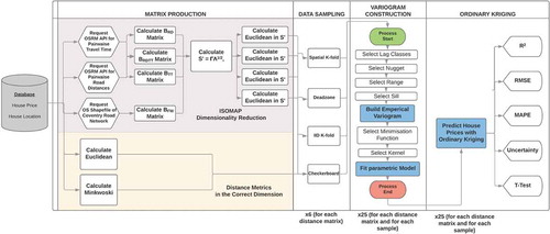
To this end, we build a so-called AVM for a sample of 3669 residential properties in the city of Coventry in the United Kingdom, using Ordinary Kriging with a target valuation date of 1 January 2017. We develop a new approximate road distance and travel time metric for variogram calculations. Figure 3 diagrammatically depicts the entire process in this study and Algorithm 1 represents the purple coloured section of the diagram.

Algorithm 1. Pseudocode for the entire isomap algorithm displayed in the purple coloured section of Figure 3.

Figure 1. A comparison of the actual road, Euclidean, Minkowski and Manhattan distances between two points on a map (OpenStreetMap Contributors 2008).

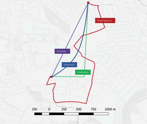
Figure 2. Illustration of the spatial transformation from road distance (or travel time) into a Euclidean space.

Figure 3. A flow diagram diagrammatically depicting the entire experimental process for the UK real-estate valuation case study described in this paper.

Require: $D=\left\{d_{ij}\right\}$, $\zeta =(s,d{)}_i$, $x$, Floyd–Warshall, $B_{ij}^{+}$, $B_{ij}^{\ast }$, $B_{ij}^{2+}$, $\kappa$, S.

1:  for experiment in 3–6 do

2:    Let: $\zeta =(s,d{)}_i$ be a metric space with point set $s=(s_1,s_2,\dots ,s_n{)}_i$ and distancefunction $d$ and $x=x_n$ is the point set of midpoints for each vertex.

3:    if {i = 3}

4:    $D=\left\{d_{ij}\right\}$ $\leftarrow$ Floyd–Warshall

5:    Map D to a semi-PD distance metric with Eq. (5)

6:    else if {i = 4,5}

7:    $D=\left\{d_{ij}\right\}$ $\leftarrow$ OSRM restricted road distance, travel time

8:    Map D to a semi-PD distance metric with Eq. (7) ($r<n$)

9:    else

10:    $D=\left\{d_{ij}\right\}$ $\leftarrow$ OSRM restricted road distance, travel time

11:    Map D to a semi-PD distance metric with Eq. (8) ($r<n$)

12:    end if

13:    Embed into low-dimensional Euclidean space ${\zeta }^{\prime }=(s^{\prime },d^{\prime }{)}_i$ such that $\alpha <r$ (Eq. 6)

14:    Collect new coordinates $s^{\prime }$ given $S^{\prime }$ in ${\zeta }^{\prime }$

15:    Calculate the new Euclidean distances

16:  end for

For the purpose of comparison, and to ensure robust results, we run six experiments where each contains a different input distance metric:

1. Euclidean (vector norm of 2);

2. Optimal Minkowski (P = 1.6) Crosby17;

3. FW on a road network (PD Road) HaixongDistanceMatric;

4. OSM road distance with restrictions;

5. OSM travel time with restrictions;

6. A combination of normalised road distance and travel time with restrictions.

Each experiment is subsequently referred to using the numerical identifier (1–6).

5.1. Data description

Our AVM uses input data regarding all houses that were sold in Coventry in 2016. For each of these 3669 properties, the percentage change in house price, between the date sold and 1 January 2017, is calculated using the predicted change in value in each output area as defined by the UK Office for National Statistics. This provides a predicted price per property for the data as at the 1 January 2017.

The datasets that we use are all open source. The house prices are obtained from Her Majesty’s Land Registry. In addition, experiment (3) requires road network data, which is also sourced from the Ordnance Survey. Experiments (4)–(6) all require distances between points along a roadway and the time that it takes to travel these distances; this is sourced from the Open Street Routing Machine (OSRM) powered by OSMs. Table 1 provides a description of each dataset and Table 2 lists roadway restrictions routinely used in the calculations by the OSRM.

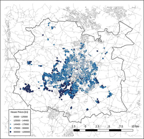
Figure 4 provides a graphical representation of all house prices from a low price (small, light-coloured circles) to a high price (large, dark-coloured circles). Empirically, it can be seen that the south west of the city of Coventry has a larger proportion of more expensive houses compared with the north east; hence, there exists some global spatial autocorrelation (SAC). Formally, a standard Moran’s I test was implemented (see definition by Moran 1950) to confirm a statistically significant SAC. This dataset showed a strong result for $I_{observed}=0.1559136>>I_{expected}=-0.00267094$, with a standard deviation of $0.001123158$ and a P-value $\simeq 0$. These results allow us to reject the null hypothesis that there is no SAC present at $\alpha$ = $0.05$. This result supports the notion that spatial regression is appropriate for our application.

Figure 4. A plot of all locations and prices in the houses dataset. Small and light points represent cheaper houses and large dark points represent the more expensive.

5.2. Matrix construction

We process five distance matrices for our six experiments. Experiments (1) and (2) require a Euclidean and a Minkowski distance metric, respectively, which are valid for variogram modelling (see the beige-coloured portion of Figure 3). Experiment (2) uses a P-value of 1.6 which was previously reported to perform best on the same dataset, see Crosby et al. (2018). Experiments (3)–(6) require pre-processing using isomap (see purple-coloured portion of Figure 3). Experiment (3) utilises a road network to calculate a shortest path using the FW algorithm. Experiment (3) embeds the input distance matrix using dissimilarity matrix $B^{\ast }$. Experiments (4) and (5) embed the distance matrices sourced from OSRM and dissimilarity $B^{+}$. Finally, experiment (6) utilises the same distance matrices sourced from OSRM but now implementing the $B^{2+}$ dissimilarity matrix. This entire process is depicted in the matrix production column in Figure 3, the purple-coloured portion of which is captured in Algorithm 1 and used in experiments (3)–(6). Table 3 provides a comparison of all distance metrics calculated in our experiment compared with OSRM's actual road distance and travel time matrices.

5.3. Data sampling for cross-validation

The most sophisticated validation sampling techniques (hold-out and $k$-fold) assume data in both the test and training sets to be independent of each other. This is an assumption that may be unrealistic with datasets containing SAC, especially if the purpose of the modelling is for interpolation or close proximity extrapolation (Pohjankukka et al. 2017). As such, four sampling techniques are considered, three of which consider spatial dependence for comparison (see ‘data sampling’ in Figure 3):

1. 10-Fold cross-validation on the full dataset of 3669 properties;

2. spatially stratified 10-fold cross-validation (spatially stratified k-fold cross-validation [SSKCV]) on the full dataset of 3669;

3. chequerboard holdout on a training set of 1832 properties, with a test set of 1837 properties;

4. spatial k-fold cross-validation (SKCV) (Pohjankukka et al. 2017) on samples of the entire dataset, with each sample including 3187 properties $\pm$ 135 for each fold.

5.3.1. k-Fold cross-validation

k-Fold cross-validation (KCV) randomly partitions a dataset into $k$ equally sized subsets. One of these subsets is retained for testing, whereas the other k − 1 are considered for training. For each fold, a different subset is retained for testing until all $k$ subsets are tested. Figure 5(e,f) shows 2 of the 10-folds in our 6 experiments. KCV overestimates statistical effects on spatial random variables and hence produces an optimistic estimate of generalisation performance for unseen data.

Figure 5. A comparison of all sampling techniques: (a) chequerboard holdout: training points (black grid) and testing points (white grid); (b) spatial k-fold with dead-zone radii: yellow points are removed from the training set; (c) blue points are the training set and brown points are the test set, spatial K = 1; (d) blue points are the training set and brown points are the test set, spatial K = 2; (e) blue points are the training set and brown points are the test set, standard K = 1; and (f) blue points are the training set and brown points are the test set, standard K = 2.

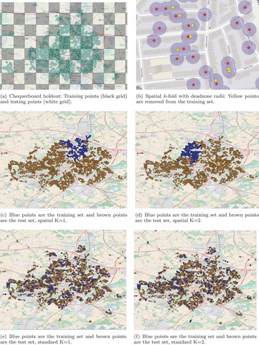
5.3.2. Chequerboard holdout

Chequerboard holdout trains approximately 50% of the data and tests the remaining data based on whether they lay in the black or white grid squares (see Figure 5(a)). Our case study uses a training and test set of 1832 and 1837 properties, respectively. Chequerboard holdout is quick to apply, simple and removes some SAC. On the other hand, it removes a significant amount of training data and still contains bias at block borders.

5.3.3. SSKCV

SSKCV processes data in a similar manner to standard k-fold; however, the data splits are spatial and not random. Two of the 10-folds are shown in Figure 5(c,d). As can be seen, each test subset is spatially separated from the training set, which can appropriately remove some bias caused by SAC. However, the data splits still contain SAC at and near sample borders.

5.3.4. SKCV

SKCV estimates a predictor’s performance by implementing traditional k-fold cross-validation, whilst at the same time removing all training points within an empirically designed Euclidean dead zone from all test points (Pohjankukka et al. 2017). Figure 5(b) demonstrates this method where training points within 20 m of each test point are in yellow for a specific fold. This method more efficiently removes SAC than the other methods. However, it relies on a user-defined dead zone with no given heuristic and removes training points which in turn can cause pessimistic results. For our case study, we apply 20 m dead-zones, which removes approximately 8% of the total training points: this parameter value is selected as it is at this level that we see the most significant change in results; close inspection shows that this removes on average 3–5 of properties’ closest neighbours.

5.4. Variogram construction and ordinary Kriging

Let $s\in {\mathbb{R}}^d$ be a single location representing a house in a d-dimensional Euclidean space and suppose that the house price Z($s$) at spatial location $s$ is a random quantity. Then, let $s$ vary over index set $D$, which is a subset of ${\mathbb{R}}^d$ ($D\subset {\mathbb{R}}^d$), so as to generate the random process $\mathbf{Z}(s):s\in D$.

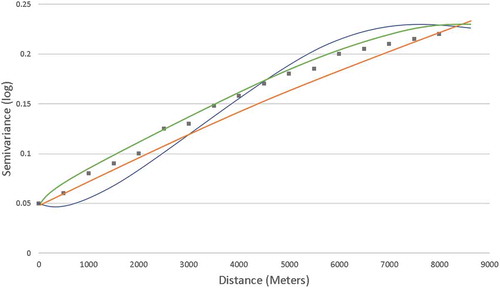
For each experiment (six in total) and each sampling technique (four in total), a new variogram is produced together with a parametric model (kernel); see ‘variogram construction’ in Figure 3. The maximum distance and lag classes are empirically selected. The nugget, sill and range are selected by ordinary least squares. For each fold in a k-fold sampling technique, a new variogram is estimated. By means of an example, Figure 6 graphically displays the variogram for the first fold of experiment (4) (restricted road distance metric) with its three best performing kernels: Gaussian, spherical and Matern (in improving order). We undertake two approaches to selecting the best variogram: (1) the user empirically selects the kernel; and (2) a maximum likelihood estimator (MLE) selects the best kernel (Lark 2002). We find that the empirical fitting approach, although lengthy to undertake, produces in all cases a matching or better predictor result. Hence, Section 5.6 reports the optimal results with empirical fitting for all sampling techniques as well as MLE for k-fold cross-validation as evidence that we selected the best approach. Table 4 provides the selected parameters and hyperparameters for each experiment with our most realistic sampling approach – SKCV. It can be seen that the kernel used can change between each experiment; this is because we select the kernel which produces the best Kriging result for each experiment. The kernels show that different distance matrices can make a significant difference to the parameters and weightings of an optimal Kriging predictor. Given that we provide the best result, irrelevant of the kernel, we are providing a more robust like-for-like comparison than we would if we just selected one kernel for all experiments. We believe that this avoids overly optimistic results for one or two experiments and pessimistic results for the remainder.

Figure 6. A graph of the three best kernels for a road distance matrix.

5.5. Validation

Three validation metrics are utilised: (1) $r^2$, (2) root mean squared error (RMSE) and (3) mean absolute percentage error (MAPE) (see Equations (10)–(12)). The $r^2$ calculation measures the predictor’s ‘goodness of fit’, the RMSE calculates the square root of the sum of the mean squared errors and MAPE is the mean absolute error expressed as a percentage.

(10) $r^2={\left(\frac{n(\sum xy)-({\sum }^x)(\sum y)}{\sqrt{(n\sum (x^2)-{(\sum x)}^2)(n\sum (y^2)-{(\sum y)}^2)}}\right)}^2.$(10)

(11) $RMSE=\sqrt{\frac{1}{n}\sum _{i=1}^n{(y_i-{\hat{y}}_i)}^2}$(11)

(12) $MAPE=\frac{100}{n}\left(\frac{\sum _{i=1}^n{\left(y_i-{\hat{y}}_i\right)}^2}{y_i}\right)$(12)

5.6. Results and analysis

A summary of all results is recorded in Table 5, which provides the validation results for each experiment (1–6) for all validation techniques (k-fold, chequerboard, SSKCV and SKCV). All values in bold represent the experiment which provides the best house price predictor for each sampling technique. If more than one experiment is selected for one sampling technique, then all results between are statistically insignificant based on a t-value of 0.05 on a paired t-test, and hence, all are optimal. It can be seen that prior state-of-the-art Euclidean and Minkowski consistently under-perform compared with the urban road distance and travel time-based models. For example, Euclidean-based Kriging delivers an $r^2$ of 0.23 compared with a combination of road distance and travel time of $r^2$ of 0.56 (>x² goodness of fit) on the most pessimistic/realistic sampling technique (SKCV). In addition, we note that by considering the shortest path with restrictions (i.e. experiments (4)–(6)), unlike the current state of the art in isomap (experiment (3)), we are able to find a statistically improved house price regression in 3 out of 4 sampling techniques.

Notably, the significance of the improvements between our new approaches (experiments (4)–(6)) compared to Euclidean distances increases as the sampling technique becomes more pessimistic. This is intuitive because in SKCV, a Euclidean dead zone is utilised to penalise the over bias caused by SAC. Additionally, our novel approaches take account of a more sophisticated SAC which better infers the covariates of an urban environment and hence is less affected by the assumption of independent and identically distritributed (IID) in k-fold cross-validation.

As previously discussed (Section 5.4), Table 6 presents the results for all experiments with a MLE. These are inferior to the empirical approach; hence, we opted to undertake all experiments with the empirical approach; these results are shown in Table 5. Table 7 emphasises this point by reporting that our empirically selected kernels produce improved urban house price Kriging predictors compared with the MLE approach undertaken in Crosby et al. (2018).

Table 6. Maximum likelihood results with dead zone spatial k-fold cross-validation.

	Euclidean distance (Exp. 1)	Minkowski distance (Exp. 2)	PD road HaixongDistanceMatric (Exp. 3)	Road distance (Exp. 4)	Travel time (Exp. 5)	Combined matrices (Exp. 6)
$r^2$	0.187	0.236	0.431	0.413	0.327	0.457
$RMSE$	102,155.62	108,238	91,047	94,655.37	104,157	92,051
$MAPE$	32.60	33.25	36.01	29.62	27.79	28.04

Table 7. A comparison of the results from Crosby et al. (2018) with those from this research using 10-fold cross-validation.

	P = 2 New	P = 2 Crosby17	P = 1.6 New	P = 1.6 Crosby17
$r^2$	0.801	0.663	0.8	0.6901
$RMSE$	55,177	58,913	74,786	57,013
$MAPE$	17.9%	18.12%	24.5%	17.895%

Overall, we see that our isomap approach can, in some cases, deliver a goodness of fit which is twice as good as results from an approach using Euclidean distance. This statistically significant outcome highlights the potential of using restricted road distance, travel time and non-Euclidean distance matrices, in urban studies and in other geostatistical applications such as restricted stream distances.

Isomap is representative of a network’s global structure and is theoretically understood across disciplines. Local isometric embedding, on the other hand, attempts to preserve the local geometry of data; these methods include sparse matrix computations that speed up calculation and utilise local geometry and Euclidean distances in a network, which may otherwise be non-Euclidean globally. Given that we have utilised the commonly understood global approach, further research would include testing against local isometric embedding, especially if one were interested in producing real-time applications which require a low computational complexity.

6. Conclusion

Through the use of a practical urban modelling case study, we demonstrate that variogram functions do not always remain valid with non-Euclidean distance inputs, and therefore establishing the validity of each distance function becomes essential. Using isomapping – a method for nonlinear dimensionality reduction – we show that it is possible to produce PD Euclidean distance metrics, and as a result valid variogram functions.

In contrast to previous research, we demonstrate that shortest path link-based road distances do not always improve the output of geostatistical models compared with Euclidean-based approaches. However, road networks which consider real-world restrictions, such as one-way systems, congestion and the presence of traffic lights can significantly improve modelling accuracy. Two such approaches presented in this research are travel time and a combination of restricted road distance and travel time, the latter of which accounts for a greater number of factors than road distance alone.

More specifically, a newly defined isomap approach is presented, which shows that road distance and travel time can both be more accurately modelled against a PD approximation of both, compared to Euclidean, Minkowski and link-based approaches (Zou et al. 2012, Crosby et al. 2018). In some cases, this provides a goodness-of-fit value which is twice as good as state-of-the-art approaches.

Furthermore, an extensive comparison of spatial cross-validation techniques is conducted, in which we conclude that k-fold cross-validation does not accurately estimate how well a model generalises to unseen data in a spatial setting – SKCV is shown to be a more appropriate sampling technique for cross-validation.

We highlight that using an inappropriate validation sampling technique can lead to an incorrect selection of prediction models. In the case study that we present, the results for our combined road distance and travel time method are significantly better with SAC removal than with standard k-fold cross-validation. Our results show that restricted road distance and travel time predictions produce a statistically improved house price predictor with an $r^2$ = 0.56; this compares with a Euclidean-based approach which achieves a result of $r^2$ = 0.23 in the case of sampling with a pessimistic/realistic dead-zone k-fold cross-validation technique (SKCV).

Further avenues of research include the introduction of covariates for an optimal AVM, the production of a restricted road distance and travel time kernel for urban variogram modelling, and an improved estimate of combined road distance and travel time metrics.

Acknowledgements

We would like to thank the Engineering and Physical Sciences Research Council (EPSRC) Centre for Doctoral Training in Urban Science (EP/L016400/1) and the Alan Turing Institute (EP/N510129/1) grants. In addition, we are supported by the Lloyd’s Register Foundation programme on Data Centric Engineering. Finally, our gratitude goes to all the open source mapping contributors.

Disclosure statement

No potential conflict of interest was reported by the authors.

Additional information

Funding

This work was supported by the Engineering and Physical Sciences Research Council: [Grant Number EP/L016400/1 and EP/N510129/1].

Notes on contributors

Henry Crosby

Henry Crosby is a PhD candidate at the Centre for Doctoral Training in Urban Science in the Warwick Institute for the Science of Cities. He received his BSc (Hons) degree in Business and Mathematics from Aston University, United Kingdom, and his MSc in data analysis at the University of Warwick.

Theodore Damoulas

Theodore Damoulas is an associate professor in Data Science with a joint appointment in the Department of Statistics and Department of Computer Science at the University of Warwick. He is also a Turing Fellow of the Alan Turing Institute and affiliated with NYU as a visiting exchangeprofessor at the Center for Urban Science and Progress (CUSP). Previously, he was a research associate at Cornell University. His studies were undertaken at the University of Edinburgh, Manchester and Paul Scherrer Institut, Switzerland.

Stephen A. Jarvis

Stephen A. Jarvis studied at London, Oxford and Durham Universities before taking his first lectureship at the Oxford University Computing Laboratory. After a short secondment to Microsoft Research in Cambridge, he joined the University of Warwick, rising to professor in 2009. He acted as Director of Research from 2008 to 2013 at which point he was appointed chair of department. Professor Jarvis is a visiting exchange professor at New York University and is engaged with the Alan Turing Institute. He is presently deputy pro vice chancellor (research) at the University of Warwick.

References

- Banerjee, S., 2005. On geodetic distance computations in spatial modeling. Biometrics, 61 (2), 617–625. doi:10.1111/biom.2005.61.issue-2
- Basu, S. and Thibodeau, T.G., 1998. Analysis of spatial autocorrelation in house prices. The Journal of Real Estate Finance and Economics, 17 (1), 61–85. doi:10.1023/A:1007703229507
- Biello, D., 2012. Gigalopolises: urban land area may triple by 2030. Scientific American, https://www.scientificamerican.com/article/cities-may-triple-in-size-by-2030/.
- Champion, T., 2014. People in cities: the numbers. Future of cities: working paper. Foresight, Government Office for Science.
- Changling, W.G.G., 1987. Application of the Kriging technique in geography. Acta Geographica Sinica, 4, 008.
- Crawford, C.A.G. and Young, L.J., 2008. Geostatistics: whats hot, whats not, and other food for thought. In: Proceedings of the 8th International Symposium on Spatial Accuracy Assessment in Natural Resources and Environmental Sciences, Shanghai, PR China, 8–16.
- Cressie, N., 1985. Fitting variogram models by weighted least squares. Journal of the International Association for Mathematical Geology, 17 (5), 563–586. doi:10.1007/BF01032109
- Cressie, N., 2015. Statistics for spatial data. Hoboken, NJ: John Wiley & Sons.
- Crosby, H., et al., 2016. A spatio-temporal, Gaussian process regression, real-estate price predictor. In: Proceedings of the 24th ACM SIGSPATIAL International Conference on Advances in Geographic Information Systems, San Francisco, WA, USA, p. 68.
- Crosby, H., et al. 2018. Road distance and travel time for an improved house price kriging predictor. Geo-Spatial Information Science, 21 (03), 185–194. doi:10.1080/10095020.2018.1503775
- Curriero, F.C., 2005. On the use of non-Euclidean isotropy in geostatistics. Baltimore, MD: Johns Hopkins University, Department of Biostatistics Working Papers.
- Curriero, F.C., 2006. On the use of non-Euclidean distance measures in geostatistics. Mathematical Geology, 38 (8), 907–926. doi:10.1007/s11004-006-9055-7
- Dubin, R.A., 1988. Estimation of regression coefficients in the presence of spatially autocorrelated error terms. The Review of Economics and Statistics, 70 (3), 466–474. doi:10.2307/1926785
- Ganio, L.M., Torgersen, C.E., and Gresswell, R.E., 2005. A geostatistical approach for describing spatial pattern in stream networks. Frontiers in Ecology and the Environment, 3 (3), 138–144. doi:10.1890/1540-9295(2005)003[0138:AGAFDS]2.0.CO;2
- Garcıa-Soidán, P.H., Febrero-Bande, M., and González-Manteiga, W., 2004. Nonparametric kernel estimation of an isotropic variogram. Journal of Statistical Planning and Inference, 121 (1), 65–92. doi:10.1016/S0378-3758(02)00507-4
- Gayle, D., 2017. Daily commute of two hours reality for 3.7m UK workers. The Guardian UK. Work Life Balance.
- Henretty, N., 2018. Housing affordability in England and Wales: 2017. Manchester: Office of National Statistics.
- Houlden, V., Weich, S., and Jarvis, S., 2017. A cross-sectional analysis of green space prevalence and mental wellbeing in England. BMC Public Health, 17 (1), 460. doi:10.1186/s12889-017-4401-x
- Huang, B., Wu, B., and Barry, M., 2010. Geographically and temporally weighted regression for modeling spatio-temporal variation in house prices. International Journal of Geographical Information Science, 24 (3), 383–401. doi:10.1080/13658810802672469
- Hudson, G. and Wackernagel, H., 1994. Mapping temperature using kriging with external drift: theory and an example from Scotland. International Journal of Climatology, 14 (1), 77–91. doi:10.1002/(ISSN)1097-0088
- Kok, N., Monkkonen, P., and Quigley, J.M., 2011. Economic geography, jobs, and regulations: the value of land and housing. In: AREUEA Meetings Denver, Denver, USA.
- Lark, R., 2002. Optimized spatial sampling of soil for estimation of the variogram by maximum likelihood. Geoderma, 105 (1–2), 49–80. doi:10.1016/S0016-7061(01)00092-1
- Liebig, T., et al., 2014. Predictive trip planning-smart routing in smart cities. In: EDBT/ICDT Workshops, Athens, Greece, 331–338.
- Little, L.S., Edwards, D., and Porter, D.E., 1997. Kriging in estuaries: as the crow flies, or as the fish swims? Journal of Experimental Marine Biology and Ecology, 213 (1), 1–11. doi:10.1016/S0022-0981(97)00006-3
- Lu, B., et al. 2014. Geographically weighted regression with a non-Euclidean distance metric: a case study using hedonic house price data. International Journal of Geographical Information Science, 28 (4), 660–681. doi:10.1080/13658816.2013.865739
- Matheron, G., 1963. Principles of geostatistics. Economic Geology, 1246–1266. doi:10.2113/gsecongeo.58.8.1246
- Miura, H., 2010. A study of travel time prediction using universal kriging. Top, 18 (1), 257–270. doi:10.1007/s11750-009-0103-6
- Moran, P.A., 1950. Notes on continuous stochastic phenomena. Biometrika, 37 (1/2), 17–23. doi:10.1093/biomet/37.1-2.17
- Murphy, R.R., et al. 2014. Water-distance-based kriging in Chesapeake Bay. Journal of Hydrologic Engineering, 20 (9), 05014034. doi:10.1061/(ASCE)HE.1943-5584.0001135
- Nations, U., 2016. The Worlds City’s in 2016. World Urbanization Prospects Report ISBN 978-92-1-151549-7, Department of Economic and Social Affairs, United Nations.
- OpenStreetMap Contributors, 2008. OpenStreetMap: user-generated street maps. IEEE Pervasive Computing, 7 (4), 12–18. doi:10.1109/MPRV.2008.80
- Pace, R.K., et al. 1998. Spatiotemporal autoregressive models of neighborhood effects. The Journal of Real Estate Finance and Economics, 17 (1), 15–33. doi:10.1023/A:1007799028599
- Pohjankukka, J., et al. 2017. Estimating the prediction performance of spatial models via spatial k-fold cross validation. International Journal of Geographical Information Science, 31 (10), 2001–2019. doi:10.1080/13658816.2017.1346255
- Seto, K.C., Güneralp, B., and Hutyra, L.R., 2012. Global forecasts of urban expansion to 2030 and direct impacts on biodiversity and carbon pools. Proceedings of the National Academy of Sciences, 109 (40), 16083–16088. doi:10.1073/pnas.1211658109
- Stewart, S., et al. 2003. Heart failure and the aging population: an increasing burden in the 21st century? Heart (British Cardiac Society), 89 (1), 49–53. doi:10.1136/heart.89.1.49
- Tenenbaum, J.B., De Silva, V., and Langford, J.C., 2000. A global geometric framework for nonlinear dimensionality reduction. Science, 290 (5500), 2319–2323. doi:10.1126/science.290.5500.2319
- Thaler, R., 1978. A note on the value of crime control: evidence from the property market. Journal of Urban Economics, 5 (1), 137–145. doi:10.1016/0094-1190(78)90042-6
- Theodoridou, P.G., et al., 2015. Geostatistical analysis of groundwater level using Euclidean and non-Euclidean distance metrics and variable variogram fitting criteria. In: EGU General Assembly Conference Abstracts, Vienna, Austria, Vol. 17.
- Townsend, A., 2015. Cities of data: examining the new urban science. Public Culture, 27 (2 (76)), 201–212. doi:10.1215/08992363-2841808
- Yu, K., Mateu, J., and Porcu, E., 2007. A kernel-based method for nonparametric estimation of variograms. Statistica Neerlandica, 61 (2), 173–197. doi:10.1111/stan.2007.61.issue-2
- Zou, H., et al. 2012. An improved distance metric for the interpolation of link-based traffic data using kriging: a case study of a large-scale urban road network. International Journal of Geographical Information Science, 26 (4), 667–689. doi:10.1080/13658816.2011.609488