An experimental analysis of least-cost path models on ordinal-scaled raster surfaces

ABSTRACT

Selection of optimal paths or sequences of cells from a grid of cells is one of the most basic functions of raster-based geographic information systems. For this function to work, it is often assumed that the optimality of a path can be evaluated by the sum of the weighted lengths of all its segments – weighted, i.e. by the underlying cell values. The validity of this assumption must be questioned, however, if those values are measured on a scale that does not permit arithmetic operations. Through computational experiments with randomly generated artificial landscapes, this paper compares two models, minisum and minimax path models, which aggregate the values of the cells associated with a path using the sum function and the maximum function, respectively. Results suggest that the minisum path model is effective if the path search can be translated into the conventional least-cost path problem, which aims to find a path with the minimum cost-weighted length between two terminuses on a ratio-scaled raster cost surface. On the other hand, the minimax path model is found mathematically sounder if the cost values are measured on an ordinal scale and practically useful if the problem is concerned not with the minimization of cost but with the maximization of some desirable condition such as suitability.

KEYWORDS:

• Least-cost paths
• raster cost surfaces/suitability surfaces
• shortest path problem
• lexicographic preference
• scales of measurement

1. Introduction

Geographic information systems (GIS) are frequently used by planners to facilitate land evaluation, which is a process of evaluating each piece of land in a given study area for a certain use and precedes a process of selecting one or more candidate sites for that use (see, e.g. Jankowski and Richard (1994), Malczewski (2004), and Church and Murray (2008) for reviews on land evaluation and site selection within a GIS platform). If a raster-based GIS is used, land evaluation can be seen as ‘transformation of one or more sets of values associated with a grid of cells into another set of such values through a function reflecting one or more criteria’ (Murekatete and Shirabe 2018). Its output is a raster surface of ‘suitability’ or ‘cost’ (depending on context), which often takes numerical values within a set range.

Planners may find a cost surface particularly useful if they seek a path and aim to minimize some kind of cost (or risk or any other undesirable consequence) associated with its location. This is because the search for a least-cost path on a cost surface can be easily cast as the problem of finding the shortest path in a graph by equating cells and pairs of adjacent cells with nodes and arcs, respectively, and there are efficient algorithms (e.g., most notably Dijkstra’s (1959) and its variants) for its solution. A variety of applications of raster least-cost path models are found in the literature, some concerning right-of-ways for large-scale infrastructures such as highways (Lombard and Church 1993, Yu et al. 2003, Scaparra et al. 2014), power lines (Huber and Church 1985, Monteiro et al. 2005, Bagli et al. 2011) and pipelines (Feldman et al. 1995, Kang and Lee 2017) and others concerning conservation corridors for wildlife (Adriaensen et al. 2003, Chetkiewicz and Boyce 2009, Rayfield et al. 2010). Here we point out one nontrivial assumption that a least-cost path model, implicitly or explicitly, relies on. That is, no matter what cost is considered, it is measured on a scale such that the aggregation of individual cost values, e.g., by addition or multiplication, is meaningful. To see this, consider a typical cost surface on which a value is assigned to each cell indicating a cost per unit length within that cell. Then the cost of a line segment contained in a cell can be calculated as the product of the length of that line segment and the value of that cell, and the cost of a sequence of such line segments given by the sum of their ‘cost-weighted’ lengths.

The quantification of cost is often done by reclassifying land cover types (e.g., Ray et al. 2002, Chardon et al. 2003, Nikolakaki 2004, Kautz et al. 2006, Driezen et al. 2007, Stevenson-Holt et al. 2014, Ziółkowska et al. 2014). Alternatively, cost is parameterized into multiple environmental variables (e.g., vegetation, slope, and proximity to targets) whose relationships may be defined according to expert opinions (e.g., Knaapen et al. 1992, Chardon et al. 2003, Gonzales and Gergel 2007, LaRue and Nielsen 2008, Spear et al. 2010). In another frequently used approach, cost is inversely or negatively related to some advantageous quality generally referred to as ‘suitability’ (e.g., Ferreras 2001, Wang et al. 2008, Chetkiewicz and Boyce 2009, Poor et al. 2012, Trainor et al. (2013), Reding et al. (2013), Ziółkowska et al. 2014) assuming that if a location is less suitable for a certain use, it will cost more to use that location for that use. In any case, cost is nothing but an estimate from supposedly relevant data with various degrees of uncertainty and subjectivity (see, e.g., Beier et al. (2008), Rayfield et al. (2010), Spear et al. (2010), Zeller et al. (2012), Ligmann-Zielinska and Jankowski (2014) for reviews).

The assumption noted above is clearly satisfied if cost is measured on a ratio scale. Cost of driving in US dollars per mile (Hallett and McDermott 2011), inverse of travel speed in minutes per meter (Mulrooney et al. 2017), and energy expense per unit distance (Ray et al. 2002) are such examples. There are cases, however, in which cost values, though encoded numerically, only reflect their rank order, and their differences are defined arbitrarily. How ranks are numbered depends on the application or the convention of the domain to which it belongs. For example, Graham (2001) assigned 1, 2, and 3 as cost values to three land cover classes in the reverse order of habitat suitability for keel-billed toucans. As another example, Rabinowitz and Zeller (2010) assigned the integers from 0 to 10 to ‘no cost’ to ‘high cost’ for the jaguar movement.

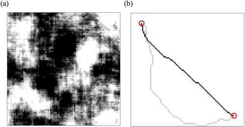
It is true that a commercial GIS accepts an ordinal-scaled cost surface (as long as numerically encoded) as input to its least-cost path function. It is generally known, however, that the location of a least-cost path on a cost surface is affected by the range or increment of cost values (e.g. Schadt et al. 2002, Larkin et al. 2004, Driezen et al. 2007, Gonzales and Gergel 2007, Rayfield et al. 2010, Murekatete and Shirabe 2018) and also by the definition (or location) of the zero cost value, which determines the relative differences of cost values. To illustrate the latter effect (which may be less obvious), let us take a raster surface consisting of 10 classes as shown in Figure 1(a), assign those classes two sets of consecutive integers, 1–10 and 11–20, as cost values, and find, for each set, a least-cost path between a common pair of cells. It may seem counterintuitive but we have two different least-cost paths; more specifically, the one associated with the 11–20 range is straighter than the one associated with the 1–10 as seen in Figure 1(b). This is actually a result of a systematic bias and, as discussed in the next section, may well arise when the conventional least-cost path model is applied to a cost surface converted from a suitability surface.

Figure 1. (a) A 100-by-100 raster surface consisting of 10 different classes, to which two sets of cost values, 1 to 10 and 11 to 20, are assigned. Note that darker cells have higher cost values. (b) Two least-cost paths between two terminal cells (circled) on the cost surface with the different sets of values. The path generated with the cost values of 1 to 10 (lightly shaded) deviates from that with the cost values of 11 to 20 (darkly shaded)

This leads to our research questions: is there a more mathematically sound and consistent approach to evaluating the quality of a path and finding a path that optimizes that quality, when no information is available on the location of the zero cost (or suitability) value, the difference between cost (or suitability) values, or the conversion between cost and suitability values? If so, what is its practical utility compared with the conventional approach? To our best knowledge, most of the relevant studies found in the literature focus on the sensitivity of the location of least-cost paths to changes in (spatial or non-spatial) distribution of cost values rather than to changes in optimization function or model.

The purpose of the paper is therefore to provide a theoretical account for how the use of the conventional least-cost path model can be problematic and present an alternative to it, and compare their merits and limits through a series of computational experiments with a number of randomly generated hypothetical cost or suitability surfaces. The remainder of the paper is structured as follows. Section 2 reviews theories underlying the evaluation and optimization of paths. Section 3 describes the procedures of the experiments, whose results are reported in Section 4. Section 5 summarizes major findings from the experiments and discusses their implications.

2. Evaluation and optimization of paths

2.1. Shortest path problem

Given a network of a set of n nodes and a set of m arcs, each with an associated length, the problem of finding a path from a node designated as the origin to another designated as the destination such that the sum of the lengths of its arcs is minimized is known as the shortest path problem. Many algorithms have been developed for its solution and the best-known is perhaps the one proposed by Dijkstra (1959). In its original form, Dijkstra’s algorithm solves the shortest path problem in $O\left(n^2\right)$ time. Its runtime efficiency can be improved in theory with special data structures such as the ‘Fibonacci heap’ (Gabow et al. 1986) to $O\left(nlogn+m\right)$ time or in practice with heuristic techniques such as the ‘search algorithm A*’ (Hart et al. 1968).

2.2. Variants of shortest path problem

While it is most common to define the length of a path as the sum of the lengths of its arcs, it is possible to use other functions to aggregate those lengths. The max and min functions are two alternatives. The use of the max function redefines the length of a path as the greatest length of any arc of the path and modifies the shortest path problem to the ‘minimax path’ problem (Oded and Handler 1987), which can be solved by Dijkstra’s algorithm with little modification. If the problem is considered in an undirected network, it can be solved in $O\left(m\right)$ time by repeating a depth-first search (DFS) for a feasible path in each progressively reduced subnetwork of the network (Camerini 1978).

Similarly, if the min function replaces the sum function, the length of a path is redefined as the smallest length of any arc in the path. While it is trivial (and of limited practical use) to find a path that minimizes the smallest arc length, it is worth considering maximizing the smallest arc length in the path search. The ‘maximin path’ problem as such is mathematically equivalent to the minimax path problem mentioned above and thus can be solved as well. The problem was first introduced as ‘the maximum capacity route problem’ by Pollack (1960) and may be called by different names such as ‘the bottleneck shortest path problem’ (Gabow and Tarjan 1988) and ‘the widest path problem’ (Wang and Crowcroft 1995) depending on the context. It is important to note that if the sum function were used for the aggregation of arc lengths, the maximization problem would be computationally intractable, as it is an NP-hard problem known as ‘the longest path problem’ (Lawler 1976).

2.3. Least-cost paths on raster cost surfaces

Where there are spatial entities between which adjacency and metric relationships are defined, the shortest path problem and its variants can be considered. In the case of raster space, two grid cells sharing one grid edge or one and only one grid vertex are often assumed to be (orthogonally or diagonally, respectively) adjacent to each other and a path is represented by a sequence of adjacent cells or of arcs implied by adjacent cells.

If, as is often the case with raster-based GIS, the distance between two adjacent cells is calculated as the straight-line distance between their centers multiplied by their mean value, the following formula gives the length of a path, P, on a surface, f, which is here referred to as path P’s ‘sum-f length’ and denoted by $l_{sum}\left(P,f\right)$.

(1) $l_{sum}\left(P,f\right)={\sum }_{\left(i,j\right)\in P}\left[\left(\frac{f\left(i\right)+f\left(j\right)}{2}\right)\cdot l\left(i,j\right)\right]$(1)

where $f\left(i\right)$ and $l\left(i,j\right)$ indicate the value of cell i on surface f and the straight-line distance between the centers of cells i and j, respectively.

If surface f represents the cost, the above equation is equivalent to the definition of the conventional cost(-weighted) length. Thus, what is commonly known as a least-cost path is a path that minimizes this length, and here referred to as a ‘minisum-cost path’ for consistency in our terminology.

Although it is less conventional, the optimality of path P may be evaluated in terms of the maximum value among all its cells on surface f, which is here referred to as path P’s ‘max-f length’ and denoted by $l_{max}\left(P,f\right)$. It is formally expressed by:

(2) $l_{max}\left(P,f\right)=\underset{i\in P}{max}f\left(i\right)$(2)

The problem of finding a path with the smallest max-cost length – or a ‘minimax-cost path’ in our terminology – between two terminal cells is a raster version of the minimax path problem. Minimizing the max-cost length certainly does not mean minimizing the sum-cost length but has an indirect effect of decreasing it. A real advantage of using this length in the least-cost path problem is that its solution is sensitive only to the order of cost values not their magnitudes. So, if information is not available on the absolute or relative differences between cost values, which may invalidate the use of the sum-cost length, the minimax-cost path problem is still well defined and solved.

Be aware here that when the cost is only measurable on an ordinal scale, max-cost lengths cannot be meaningfully compared by their (absolute or relative) differences. To see this, suppose that there is a cost surface having five cost values, 1, 2, 3, 4, and 5, measured on an ordinal scale, and suppose also that two paths are situated on this grid and their max-cost lengths are 2 and 4. Then, if the cost values are relabeled, say, as 1, 3, 5, 7, and 9, their max-cost lengths will change to 3 and 7. This implies that the difference between those lengths can be arbitrarily increased or decreased.

2.4. Most-suitable paths on raster suitability surfaces

There may be cases where path planners are interested not in minimizing the cost but in maximizing some desirable condition or ‘suitability’ in general. On a given raster surface that assigns each cell a value indicating the degree of suitability for a certain use at that cell, the planners might expect GIS to be able to find a ‘most-suitable’ path between any chosen cells. If, just like the least-cost counterpart, the most-suitable path is meant to be one that has the greatest sum-suitability length – or a ‘maxisum-suitability path’ in our terminology, we have the NP-hard longest path problem. The problem is in general intractable as mentioned earlier, but its raster version is trivial because a solution can be obtained by traversing all cells on the suitability surface. This is, however, not the kind of solution that would normally be expected in practice.

An alternative approach frequently found in the literature and in practice is to convert a suitability surface to a cost surface, on which a minisum-cost path is searched for as a most-suitable path. The suitability-to-cost conversion may be done by inversely or negatively relating cost and suitability (e.g. Ferreras 2001, Wang et al. 2008, Chetkiewicz and Boyce 2009). As a simple example, a set, S, of suitability values {1, 5, 9} can be reversed into a set of cost values {9, 5, 1} by the following linear function:

(3) $cost=minS+maxS-suitability$(3)

While this type of conversion is intuitive and easy to implement, it does not necessarily maintain the order of optimality of paths. To see this, with reference to Equation (3)(3) $cost=minS+maxS-suitability$(3) , consider two paths such that they have the same $l_{sum}\left(P,suitability\right)$ value but one is geometrically longer than the other. Because both paths get penalized additionally and constantly – by 10 (= 1 + 9) in the present example – for every unit length, the longer path has the greater $l_{sum}\left(P,cost\right)$ value, which contradicts the two paths’ equal optimality in terms of suitability. For the same reason, a minisum-cost path on a cost surface transformed from a suitability surface through a function involving a constant term has a systematic tendency to become straighter and less sensitive to the spatial distribution of original suitability values as the constant term becomes larger. The difference of the two paths shown in Figure 1 was actually caused by this effect, since the cost values of 11 to 20 could be seen as a result of adding 10 to each of the cost values of 1 to 10.

Therefore, no matter how a solution is generated, its optimality should be evaluated in terms of the original suitability rather than of the artificial cost derived from it. As discussed already, however, the sum-suitability length may not be a good means for this, because it monotonically increases with the geometric length and thus gives an unfair advantage to a longer path. A straightforward resolution of this bias normalizes the sum-f length of each path, P, by its geometric length to obtain path P’s ‘mean-f length.’ Letting $l_{mean}\left(P,f\right)$, denote this length, it is formally expressed by:

(4) $l_{mean}\left(P,f\right)=l_{sum}\left(P,f\right)/{\sum }_{\left(i,j\right)\in P}l\left(i,j\right)$(4)

Assuming that it is agreed that a path with a greater mean-suitability length is more suitable for the use under consideration, a question arises: how to find an optimal path in terms of this length? Is a minisum-cost path on a cost surface transformed from a suitability surface a satisfactory solution, if not optimal? Another important question is: how is suitability measured in the first place? Is it measured on a scale that makes the (absolute or relative) differences of any two values meaningful? If not, neither the sum-suitability length nor mean-suitability length is a valid metric.

These questions lead to the use of another kind of length similar to the max-f length introduced earlier to the least-cost path problem. Given a path, P, and a surface, f, it is path P’s ‘min-f length,’ denoted by $l_{min}\left(P,f\right)$ and defined by:

(5) $l_{min}\left(P,f\right)=\underset{i\in P}{min}f\left(i\right)$(5)

Certainly, the relevance of this length to the most-suitable path problem must be tested. If suitability is safely assumed to be measured on a ratio scale, it should be just fine to evaluate the optimality of a path in terms of mean-suitability length. On the other hand, if suitability is measured on an ordinal scale, min-suitability length seems to be a reasonable optimality measure. The problem of finding a path with the greatest min-suitability length – or a ‘maximin-suitability path’ in our terminology – between two terminal cells is a raster version of the maximin path problem. It is, as discussed earlier, equivalent to the well-solved minimax path problem. This means that no suitability-to-cost conversion is necessary for its solution. In fact, a maximin-suitability path on a suitability surface is a minimax-cost path on the cost surface derived from the suitability surface by Equation (3)(3) $cost=minS+maxS-suitability$(3) .

3. Method

Two experiments were conducted using random raster surfaces representing cost or suitability. The first experiment was designed to evaluate the relative performance of minisum-cost paths and minimax-cost paths. Two what-if questions were expected to be answered: (1) if the underlying cost values are measured on a ratio scale, how poor minimax-cost paths would be in terms of sum-cost length (compared with their minisum counterparts) and (2) if the underlying cost values are measured on an ordinal scale, how poor minisum-cost paths would be in terms of max-cost length (compared with their minimax counterparts)? The second experiment was designed similarly but concerned with two kinds of most-suitable paths, minisum-unsuitability paths – unsuitability, i.e. cost transformed from suitability by Equation (3)(3) $cost=minS+maxS-suitability$(3) – and maximin-suitability paths.

For these experiments, we implemented two algorithms based on Dijkstra’s, one for shortest paths and the other for minimax/maximin paths, in Java and run them on a 2.80 GHz Intel Core i7-7600 U CPU processor with 32.8 GB of RAM.

3.1. Experiment 1

3.1.1. Data

We generated two sets of 1000 random raster cost surfaces referenced to a common 200-by-200 grid but with two different spatial structures referred to as ‘cloudy’ (i.e. having values fairly continuously varying) and ‘patchy’ (i.e. comprising patches of constant values separated by distinct boundaries). The generation of these sample data was facilitated by a PYTHON software package, NLMpy, developed by Etherington et al. (2015). It allowed us to access a variety of algorithms for creating realistic neutral landscape models with different spatial configurations.

Each of the 1000 cloudy cost surfaces (see Figure 2(a,b) for examples) was generated using an NLMpy function that implements the ‘mid-point displacement method’ (Fournier et al. 1982). It takes two parameters, nRow and nCol, that specify the numbers of rows and columns and a parameter, h, that controls the level of spatial autocorrelation, and returns a grid of cells with random values ranging from 0 to 1 according to the specification. We set both nRow and nCol to 200, and h to a value randomly chosen from 0 (slightly autocorrelated) to 1 (highly autocorrelated). The output grid was then converted to a cost surface by mapping its values to equally (or as equally as possible) spaced integers defined by three parameters, each of which was randomly chosen from its respective range with an equal probability. The three parameters were (1) the number of unique cost values, numCost, ranging from 3 to 10, (2) the lowest cost value, minCost, greater than or equal to 1, and (3) the highest cost value, maxCost, smaller than or equal to 100, with condition that minCost + numCost – 1 ≤ maxCost so that all the cost values could take integers between minCost and maxCost.

Figure 2. Examples of (a) and (b) cloudy cost surfaces and (c) and (d) patchy cost surfaces. Note that darker shades represent higher values

Each of the 1000 patchy cost surfaces (see Figure 2(c,d) for examples) was generated using NLMpy’s ‘random cluster nearest-neighbor algorithm.’ It randomly divides a grid of specified dimensions (i.e. nRow = nCol = 200 in the present experiment) into ‘irregularly shaped and reasonably consistently sized patches’ (Etherington et al. 2015) and randomly assigns a value ranging from 0 to 1 to each patch. The algorithm takes another input parameter that controls the approximate patch size, s. We set s to an integer randomly selected from 100 cells (corresponding to 0.25% of the 200-by-200 grid) to 1111 cells (corresponding to 2.78% of the 200-by-200 grid). The output grid was then converted to a cost surface in the same manner as done for the cloudy cost surfaces using the three parameters, numCost, minCost, and maxCost.

3.1.2. Analysis

For each of the 1000 cloudy cost surfaces and the 1000 patchy cost surfaces, we randomly selected two different cells and computed a minisum-cost path and a minimax-cost path between them. It is important to note that in almost all cases, there was more than one minimax-cost path between the selected terminal cells. Many of those most likely had ‘ordinally non-dominant’ (Schäfer et al. 2020) sets of cost values – roughly, a set (or vector) of values are said to ‘ordinally dominate’ (Schäfer et al. 2020) another if each element of the former is at least as good as the corresponding element of the latter – and an enumeration of them would be tractable only in some special cases, e.g., when the underlying graph is acyclic, as assumed by Schäfer et al. (2020).

Therefore, for the present experiment, we decided to employ a tie-breaking rule, which was chosen from possible tie-breaking rules (e.g., select one arbitrarily, select one that was found first, and select one with the shortest length) that remain valid in the case of ordinal cost values. It is based on two assumptions. First, a path is more preferable than another if the former has the smaller maximum cost value than the latter. Second, if two paths have the same maximum cost value, the one with a shorter length of segments that intersect cells of that value is more preferable. If there are two or more equally preferable paths, the same assumptions hold for the kth (k = 2, 3, …) maximum cost value. That is, preference is given to one with the shortest length of segments intersecting cells with the second highest cost value, then one with the shortest length of segments intersecting cells with third highest cost value, and so on. After the last tie-break, any remaining ties are broken arbitrarily.

As shown in Appendix, the search for a path that satisfies the tie-breaker described above can be cast as an instance of the multicriteria shortest path problem with a ‘lexicographic preference relation’ (Perny and Spanjaard 2005) and solved by a modification of Dijkstra’s shortest path algorithm in polynomial time. The modified algorithm has a higher computational complexity than the original Dijkstra’s algorithm but remains reasonably efficient. In the present experiment, it took 436 seconds to generate all 2000 minimax-cost paths (i.e., approximately 0.218 seconds each), while it took 372 seconds to generate all 2000 minisum-cost paths (i.e., approximately 0.186 seconds each).

As a result, we obtained a sample of 1000 pairs of a minisum-cost path and minimax-cost path on cloudy cost surfaces, and another such sample on patchy cost surfaces. For each pair of these paths, we calculated their sum-cost lengths and max-cost lengths on their common cost surface. Obviously, by definition, the sum-cost length of the minisum-cost path was smaller than or equal to that of the minimax-cost path, and the max-cost length of the minimax-cost path was smaller than or equal to that of the minisum-cost path. Hence, our interest was the extent of their differences.

The use of sum-cost lengths assumes that cost values are measured on a ratio scale and thus allows quantification of their differences. This is not the case, however, for max-cost lengths, which are primarily used when cost values are assumed to be measured on an ordinal scale, because, as discussed in Section 2, their differences would be meaningless. Therefore, as an alternative, for each pair of a minisum-cost path and minimax-cost path, we measured the length of segments intersecting ‘undesirable’ cells, i.e. cells whose cost values were greater than or equal to the max-cost length of the minimax-cost path. In addition, we calculated their 75th percentile, 50th percentile, 25th percentile, and minimum-cost values, so that we could compare the two paths’ more comprehensive compositions of cost values. Note that the pth percentile of a path is defined herein as the cost value such that at least p% of the total length of the path intersects cells whose cost values are smaller than or equal to that cost value.

Below is an example of these characterizations using a pair of a minisum-cost path and minimax-cost path in a small cost surface illustrated in Figure 3. The max-cost length (i.e. the maximum cost value), 75th percentile, 50th percentile, and 25th percentile, and minimum-cost values of the minisum-cost path (enclosed by bold lines) are 15, 13, 7, 6, and 5, respectively. Those of the minimax-cost path (shaded) are 14, 7, 6, 5, and 5, respectively. The minisum-cost path and the minimax-cost path intersect undesirable cells (whose cost values are greater than or equal to 14) over lengths of 2.12 and 1.5, respectively.

Figure 3. (a) a minisum-cost path (enclosed by bold lines) and (b) a minimax-cost path (shaded) in a raster cost surface. Note that the number in each cell represents the cost value assigned to that cell

3.2. Experiment 2

3.2.1. Data

1000 cloudy surfaces and 1000 patchy surfaces were created in the same manner as in the first experiment, except that their values were assumed to represent suitability instead of cost. Then, we applied the suitability-to-cost conversion defined by Equation (3)(3) $cost=minS+maxS-suitability$(3) to all 2000 suitability surfaces and obtained 2000 cost surfaces, which were referred to as ‘unsuitability’ or ‘reversed suitability’ surfaces in this experiment so as to articulate what they really were.

3.2.2. Analysis

For each of the 1000 cloudy suitability surfaces and the 1000 patchy suitability surfaces, two different cells were randomly selected, and a minisum-unsuitability path and a maximin-suitability path were computed between them on the same computational platform as in the first experiment. For the latter path, we employed a tie-breaking rule and algorithm (see Appendix) similar to the one used in the first experiment, which selects a path with the shortest length of segments intersecting cells with the lowest suitability value, and if there are more than one such path, break ties by sequentially giving priority to paths with the shortest length of segments intersecting cells with the 2nd, 3rd, … lowest suitability values. It took 495 seconds to generate all 2000 maximin-suitability paths (approximately 0.248 seconds each), while it took 458 seconds to generate all 2000 minisum-unsuitability paths (approximately 0.229 seconds each).

As a result, we obtained two samples – each consisting of 1000 pairs of a minisum-unsuitability path and maximin-suitability path – one generated on cloudy suitability surfaces and the other on patchy suitability surfaces. Similarly to the first experiment, we compared each pair of these paths in terms of their mean-suitability lengths, min-suitability lengths, and lengths of segments intersecting ‘undesirable’ cells, i.e. cells whose suitability values were smaller than or equal to the min-suitability length of the maximin-suitability path. Also, we compared their maximum, 75th percentile, 50th percentile, and 25th percentile suitability values. Figure 4 shows an example of these measures using the same raster surface used in Figure 3 but assuming that its values represent suitability instead of cost. The maximum, 75th percentile, 50th percentile, and 25th percentile suitability values, and the min-suitability length (i.e. the minimum suitability value) of the minisum-unsuitability path (enclosed by bold lines) are 19, 17, 14, 8, and 5, respectively. Those of the maximin-suitability path (shaded) are 19, 16, 13, 8, and 6, respectively. The minisum-unsuitability path and the maximin-suitability path intersect undesirable cells (whose suitability values are smaller than or equal to 6) over lengths of 3.5 and 1.71, respectively.

Figure 4. (a) a minisum-unsuitability path (enclosed by bold lines) and (b) a maximin-suitability path (shaded) in a raster suitability surface. Note that the number in each cell represents the suitability value assigned to that cell

4. Results

4.1. Experiment 1

Table 1 shows partial results of the first experiment, which correspond to the first 10 (of 1000) pairs of a minisum-cost path and minimax-cost path generated on cloudy cost surfaces and those on patchy cost surfaces. The following notation is used throughout this subsection: l(minisum), l(minimax), and l(minimax)/l(minisum) represent the sum-cost length of a minisum-cost path, that of its paired minimax-cost path, and the ratio of the latter to the former, respectively; u(minisum), u(minimax), and u(minisum)/u(minimax) represent the length of segments intersecting undesirable cells in a minisum-cost path, that in its paired minimax-cost path, and the ratio of the former to the latter, respectively.

Table 1. Results of experiment 1 corresponding to the first 10 pairs of a minisum-cost path and minimax-cost path generated (a) on cloudy cost surfaces and (b) on patchy cost surfaces

(a) on cloudy cost surfaces
ID	l(minisum)	l(minimax)	l(minimax)/l(minisum)	u(minisum)	u(minimax)	u(minisum)/u(minimax)
0	5367.85	23948.80	4.46	53.55	8.50	6.30
1	6547.54	9940.37	1.52	32.50	0.71	45.96
2	9221.12	16348.73	1.77	9.71	0.50	19.41
3	17930.41	30560.30	1.70	87.65	20.31	4.31
4	12488.44	14738.97	1.18	46.54	21.85	2.13
5	14004.10	19949.95	1.42	3.50	0.50	7.00
6	3740.07	6630.79	1.77	61.96	13.12	4.72
7	10308.83	24668.78	2.39	30.24	1.00	30.24
8	3523.52	9755.05	2.77	27.44	12.71	2.16
9	15030.88	22237.88	1.48	5.71	0.50	11.41
:	:	:	:	:	:	:
(b) on patchy cost surfaces
ID	l(minisum)	l(minimax)	l(minimax)/l(minisum)	u(minisum)	u(minimax)	u(minisum)/u(minimax)
0	1923.38	3554.99	1.85	19.68	6.50	3.03
1	3887.98	8180.55	2.10	24.50	3.50	7.00
2	8238.54	15090.07	1.83	10.50	7.78	1.35
3	4574.52	4924.34	1.08	17.02	17.02	1.00
4	17957.38	21520.68	1.20	89.64	79.36	1.13
5	4232.78	33616.26	7.94	21.21	10.00	2.12
6	1357.39	1360.76	1.00	10.71	10.50	1.02
7	6511.62	8286.68	1.27	31.96	23.92	1.34
8	7888.04	17254.47	2.19	46.67	5.04	9.27
9	499.26	540.02	1.08	38.81	38.75	1.00
:	:	:	:	:	:	:

Note that ID represents the unique identifier of each pair.

As Figure 5 shows, l(minimax)/l(minisum) had a heavily right-skewed distribution. Its range, median, and mean were [1, 21.1], 1.50, 1.88, respectively, on cloudy cost surfaces, and [1, 11.1], 1.33, 1.68, respectively, on patchy cost surfaces. The minimax-cost path generally had a greater sum-cost length than its paired minisum-cost path.

Figure 5. Frequency distributions of l(minimax)/l(minisum) (a) on cloudy cost surfaces and (b) on patchy cost surfaces

As Figure 6 shows, u(minisum)/u(minimax), too, has a heavily right-skewed distribution, with its range, median, and mean being [0.37, 136], 3.01, 8.90, respectively, on cloudy cost surfaces, and [0.071, 153], 1.75, 4.39, respectively, on patchy cost surfaces. The minisum-cost path generally had longer segments intersecting undesirable cells than its paired minimax-cost path.

Figure 6. Frequency distributions of u(minisum)/u(minimax) (a) on cloudy cost surfaces and (b) on patchy cost surfaces

We regressed both l(minimax)/l(minisum) and u(minisum)/u(minimax) on each of the parameters controlling the spatial distribution (i.e. h or s) or non-spatial distributions (i.e. numCost, minCost, and maxCost) of the underlying cost surfaces. We found that their correlations with each of those parameters were weak, as the corresponding regression coefficient (or slope) and coefficient of determination (or r² s) were small.

The advantage of the minimax-cost paths over the minisum-cost paths – particularly when their associated cost values are ordinal – was evaluated also by counting the number of cases in which the maximum, 75th percentile, 50th percentile, 25th percentile, or minimum-cost value of the minimax-cost path was smaller than, equal to, or greater than that of the minisum-cost path. Those counts are presented in Table 2.

Table 2. Numbers of cases in which minimax-cost paths performed better than (1st column), equal to (2nd column), or worse than (3rd column) their paired minimum-cost path with respect to the maximum, 75th percentile, 50th percentile, 25th percentile, or minimum-cost value (a) on cloudy cost surfaces and (b) on patchy cost surfaces. (a) On cloudy cost surfaces (b) On patchy cost surfaces

(a) on cloudy cost surfaces
	Minimax < Minisum	Minimax = Minisum	Minimax > Minisum
Maximum	349	651	0
75th percentile	677	304	19
50th percentile	577	407	16
25th percentile	432	560	8
Minimum	202	797	1
(b) On patchy cost surfaces
	Minimax < Minisum	Minimax = Minisum	Minimax > Minisum
Maximum	325	675	0
75th percentile	589	376	35
50th percentile	433	504	63
25th percentile	279	683	38
Minimum	136	858	6

The top-left cell of the first table, for example, indicates that there were 349 cases in which minimax-cost paths had lower maximum cost values than their paired minisum-cost paths. The rest of the table are interpreted similarly. It was found that not only the minimax-cost path, by definition, had a lower maximum cost value than its paired minisum-cost path, but also it comprised larger proportions of lower-cost cells.

The above findings suggest that if the underlying cost values are measured on a ratio scale and sum-cost length is employed as a measure of optimality, minimax-cost paths can be significantly worse than minisum-cost paths. Likewise, if they are measured on an ordinal scale and max-cost length is chosen as the measure of optimality, minisum-cost paths can be significantly worse than minimax-cost paths. These tendencies generally hold regardless of the underlying spatial or non-spatial distribution of cost values, but to a lesser degree when the cost surface consists of patches of constant cost values.

4.2. Experiment 2

The pairwise comparison of 2000 minisum-unsuitability paths and maximin-suitability paths (summarized graphically in Figures 7 and 8) found (1) that the maximin-suitability path generally had a little longer (on average, 9% longer on cloudy suitability surfaces and 6% longer on patchy suitability surfaces) mean-suitability length than its paired minisum-unsuitability path, and (2) that the minisum-unsuitability path generally intersected undesirable cells over much longer (on average, 7.76 times longer on cloudy suitability surfaces and 4.20 times longer on patchy suitability surfaces) lengths than its paired maximin-suitability path. A regression analysis found that these tendencies did not depend on the parameters controlling the spatial or non-spatial distribution of suitability values.

Figure 7. Frequency distributions of the ratio of the mean-suitability length of a maximin-suitability path to that of its paired minisum-unsuitability path (a) on cloudy suitability surfaces and (b) on patchy suitability surfaces

Figure 8. Frequency distributions of the ratio of the length of segments intersecting undesirable cells in a minisum-unsuitability path to that in its paired maximin-suitability path (a) on cloudy suitability surfaces and (b) on patchy suitability surfaces

Another finding was that the maximin-suitability path generally comprised larger proportions of higher-cost cells than its paired minisum-unsuitability path, as shown in Table 3.

Table 3. Numbers of cases in which maximin-suitability paths performed better than (1st column), equal to (2nd column), or worse than (3rd column) their paired minimum-unsuitability path with respect to the maximum, 75th percentile, 50th percentile, 25th percentile, or minimum suitability value (a) on cloudy suitability surfaces and (b) on patchy suitability surfaces

(a) On cloudy suitability surfaces
	Maximin > Minisum	Maximin = Minisum	Maximin < Minisum
Maximum	205	794	1
75th percentile	399	592	9
50th percentile	592	391	17
25th percentile	588	382	30
Minimum	304	696	0
(b) on patchy suitability surfaces
	Maximin > Minisum	Maximin = Minisum	Maximin < Minisum
Maximum	153	844	3
75th percentile	307	637	56
50th percentile	443	495	62
25th percentile	673	312	15
Minimum	372	628	0

Note that ‘Maximin > Minisum’ represents the number of cases in which the maximin-suitability path had a better (i.e. greater) maximum, 75th percentile, 50th percentile, 25th percentile, or minimum suitability value than the minisum-unsuitability path. The two other columns are interpreted similarly.

It was also found, initially by visual inspection (see Figure 9 for examples), that the minisum-unsuitability paths were generally straighter than the maximin-suitability paths. To verify this, we calculated the sinuosity of each path as its geometric length divided by the straight-line distance between its terminal cells. The mean sinuosity of the minisum-unsuitability path was 1.12 on cloudy surfaces and 1.10 on patchy surfaces, whereas that of the maximin-suitability path was 2.37 on cloudy suitability surfaces and 1.98 on patchy suitability surfaces.

Figure 9. First two pairs of a minisum-unsuitability path (solid line) and maximin-suitability path (dashed line) and maximin-suitability path (dashed line) between two terminal cells (circled) generated (a) on cloudy cost surfaces and (b) on patchy cost surfaces. Note that darker shades represent higher values

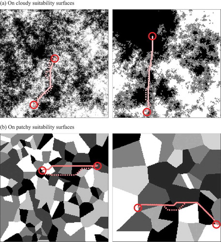
The above findings suggest that even if the underlying suitability values are measured on a ratio scale, maximin-suitability paths are likely to be fairly comparable with minisum-unsuitability paths in terms of mean-suitability length. On the other hand, if they are measured on an ordinal scale, minisum-unsuitability paths are likely to intersect unsuitable cells over longer lengths than maximin-suitability paths and suffer the ‘the-shorter-the-more-suitable’ bias.

5. Discussion and conclusions

When it is safe to assume that the value of each cell in a given raster surface is measured on a ratio scale representing the cost (or suitability) per unit distance of traversal over that cell, the conventional least-cost path model – which was referred to as the minisum-cost path model in this paper – remains a simple yet powerful tool for path planning. We argue, however, that it is worth trying or at least acknowledging alternatives that do not rely on this assumption if the value of each cell only indicates the ordinal category of cost (or suitability) of intersecting that cell. We considered the minimax-cost path model – or mathematically equivalently, the maximin-suitability path model – as one such alternative and demonstrated its merits and limits through computational experiments with artificial raster surfaces with two different spatial structures, cloudy (i.e. having values fairly continuously varying) and patchy (i.e. comprising patches of constant values separated by distinct boundaries).

One obvious advantage of the minimax-cost path model is its insensitivity to the magnitude of cost values. This allows planners to focus on which types of land are more costly for the land use under consideration, without worrying about how much or how many times more. As reported in many studies in the literature, subjectivity in the quantification of cost is a major source of uncertainty in locating the least-cost paths. Of course, if we have sufficient information on the magnitude of cost values, the evaluation of a path in terms of sum-cost length remains reasonable and so is the use of the minisum-cost path model.

The alternative model is found even more valuable when paths are searched for over a suitability surface, since it directly takes the suitability surface – on which greater values indicate higher suitability – as input and does not require an error-prone process of suitability-to-cost conversion. Unfortunately, this is not the case in the application of the minisum-cost path model to the search for most suitable paths. Furthermore, our experiments demonstrated that if the suitability-to-cost conversion has the effect of adding a positive constant, it will drive the resulting minisum-cost paths to be geometrically shorter and straighter. This tendency may not be convenient unless the minimization of geometric length is explicitly considered as a path selection criterion.

Lastly, a practical implication of this study is that there are different computational approaches to dealing with the uncertainty and subjectivity inherent in path planning. As found in the literature, trying different models of a cost (or suitability) surface – on each of which a least-cost (or most-suitable) path is searched for – is one approach. We have shown that different but equally computationally tractable models can be considered for a least-cost (or most-suitable) path, too, and applied to a given cost (or suitability) surface, which is another approach. The two approaches are not necessarily mutually exclusive but complementary to each other when planners test how their models respond to any change in their assumptions. If similar solutions are generated from different least-cost (or most-suitable) path models with different cost (or suitability) surface models, the planners can be more confident about the models’ robustness. Otherwise, the planners will obtain a pool of alternative plans, each plausible in its own way, and analyze them further possibly with additional criteria that might not be initially available. Still, we admit that this is a speculation that needs to be tested with actual problems in future studies.

Data and codes availability statement

The data and codes that support the findings of this study are available with a DOI at [https://doi.org/10.6084/m9.figshare.11800173].

Acknowledgments

The authors thank the editor and anonymous reviewers for their valuable and constructive comments on an earlier draft of the article. They also thank Dr. Thomas Etherington for his detailed explanation of models and algorithms used in the NLMpy software. Any errors remain, of course, the sole responsibility of the authors.

Disclosure statement

No potential conflict of interest was reported by the author(s).

Additional information

Funding

This work was supported by the Svenska Forskningsrådet Formas 942-2015-1513; the Swedish International Development Authority under Grant 51160059-06.

Notes on contributors

Rachel Mundeli Murekatete

Rachel Mundeli Murekatete is a PhD student in Geoinformatics at the Royal Institute of Technology (KTH), Sweden. She is also Assistant Researcher at the Centre for Geographic Information Systems and Remote Sensing (CGIS), University of Rwanda. She has a degree in geoinformation science for urban and regional planning from the University of Twente, Faculty of Geoinformation Science and Earth Observation (ITC), Netherlands. Her current research focus is on the design, evaluation and application of GIS-based spatial optimization models and methods for spatial planning practices with emphasis on raster-based model.

Takeshi Shirabe

Takeshi Shirabe is currently an Associate Professor of Geoinformatics at the Royal Institute of Technology (KTH), Sweden. He has a Ph.D. in City and Regional Planning from the University of Pennsylvania, USA and a habilitation of Geoinformation from the Vienna University of Technology, Austria. His main research area is spatial optimization and its application to planning and design.

Appendix

The ‘preferred paths problem’ (Perny and Spanjaard 2005) is a generalization of the shortest path problem whose solutions are ranked according to an arbitrary preference relation, which is not necessarily defined by a single additive scalar function. While this problem in general cannot be solved in polynomial time, there are tractable special cases that satisfy what is called the ‘independence axiom,’ such as the multicriteria shortest path problem with a ‘lexicographic preference relation’ (Perny and Spanjaard 2005).

This special case is considered in a graph in which each edge and path has a set of nonnegative lengths arranged in a certain order of preference, and the ith length of a path is defined as the sum of the ith lengths of its edges. We say that a path is preferred to another when the former is shorter than the latter in terms of one of those multiple lengths while the two paths are tied in terms of all the preceding lengths. The formulation of this preference relation is given in Example 9 of Perny and Spanjaard (2005) as follows:

A path, A, is preferred to a path, B, if and only if

(6) ${\sum }_{\left(m,n\right)\in A}{l}_k\left(m,n\right)<{\sum }_{\left(m,n\right)\in B}{l}_k\left(m,n\right)\mathrm{f}\mathrm{o}\mathrm{r}\mathrm{s}\mathrm{o}\mathrm{m}\mathrm{e}k\in I$(6)

(7) ${\sum }_{\left(m,n\right)\in A}{l}_i\left(m,n\right)={\sum }_{\left(m,n\right)\in B}{l}_i\left(m,n\right)\mathrm{f}\mathrm{o}\mathrm{r}\mathrm{a}\mathrm{l}\mathrm{l}i<k$(7)

where I represents the ordered set of indices of edge lengths, and $l_i\left(m,n\right)$ represents the ith length of an edge (m, n), i.e. edge between vertices m and n.

The multicriteria shortest path problem with the lexicographic preference relation formulated above can be solved by a modification of the classic shortest path algorithm of Dijkstra (Algorithm 1). In the original form of Dijkstra’s algorithm, a shortest path from the origin to a vertex, n, and its length, $d\left(n\right)$, are updated when the inequality $d\left(n\right)>d\left(m\right)+l\left(m,n\right)$ holds, where $l\left(m,n\right)$ is the length of edge (m, n). The modified algorithm performs a similar update when the inequality $d_k\left(n\right)>d_k\left(m\right)+l_k\left(m,n\right)$ holds for some index, k, and the equality $d_i\left(n\right)=d_i\left(m\right)+l_i\left(m,n\right)$ hold for all i < k, where $d_i\left(n\right)$ is the ith length of a shortest path from the origin to vertex n, and $l_i\left(m,n\right)$ is the ith length of edge (m, n). Pseudocode of the algorithm is presented below with the following notation.

• N represents a set of vertices.

• A(m) represents a set of vertices adjacent to vertex m.

• I represents an ordered set of edge/path length indices.

• s represents a vertex designated as the origin.

• l_i(m, n) represents the ith length of the edge between vertices m and n.

• d_i(m) represents the ith length of a path from the origin to vertex m.

• p(m) represents vertex m’s predecessor vertex.

• Algorithm 11 for each m $\in$ N

• 2 for each $i\in I$

• 3 d_i(m): = $\mathrm{\infty }$

• 4 end for

• 5 p(m):= null

• 6 end for

• 7 for each $i\in I$

• 8 d_i(s): = $0$

• 9 end for

• 10 Q: = N

• 11 while Q is not empty

• 12 find in Q a vertex, m, whose lengths are lexicographically shortest, and remove it

• 13 for each n $\in$ A(m)

• 14 for each $k\in I$

• 15 if d_k(n) > d_k(m) + l_k(m, n) then

• 16 for each $i\in I$

• 17 d_i(n): = d_i(m) + l_i(m, n)

• 18 end for

• 19 p(n):= m

• 20 break

• 21 else if d_k(n) < d_k(m) + l_k(m, n) then

• 22 break

• 23 end if

• 24 end for

• 25 end for

• 26 end while

Algorithm 1 is almost identical to Dijkstra’s algorithm, except that it initializes more than one path length for a vertex at Lines 2-3 and 7-8, searches for a vertex whose multiple lengths are lexicographically shortest at Line 12, tests the path lengths update condition for a vertex at Lines 14-15 and 21, and updates each path length for a vertex at Lines 16 to 17. These tasks require an iteration over I, which makes the complexity of Algorithm 1 $O\left({\left|N\right|}^2{\left|I\right|}^2\right)$ and higher than the complexity of Dijkstra’s algorithm, $O\left({\left|N\right|}^2\right)$.

The tie-breaking rule employed in the experiments reported in Section 3 can be considered as an instance of the lexicographic preference relation. To see this, suppose that a raster cost surface is given that contains q unique values. Then, convert it to a graph by creating a vertex for each cell and an edge for each pair of adjacent cells. Then, assign each edge (m, n) a set of q lengths in the following manner. Assume that the values of cells m and n are the rth and sth highest of the q unique values in the cost surface. If r = s, set $l_r\left(m,n\right)$ to the straight-line distance between the centers of cells m and n. If r ≠ s, set both $l_r\left(m,n\right)$ and $l_s\left(m,n\right)$ to half of the straight-line distance between the centers of cells m and n. And, in either case, set $l_i\left(m,n\right)$ to 0 for each i that is not r or s. Notice that for any path, its ith length indicates the total geometric length of subpaths that intersect cells with the ith highest value in the cost surface.

We give some examples of the calculation of edge lengths and the interpretation of path lengths with reference to the cost surface in Figure 3, which contains 19 unique values. The edge between cells at (row 1, column 1) and (row 1, column 2) has a set of 19 lengths {0, 0, 0, 0, 0, 1, 0, 0, 0, 0, 0, 0, 0, 0, 0, 0, 0, 0, 0}, as both cells have a value of 14 (the sixth highest cost value) and the distance between them is 1. The edge between cells at (row 1, column 1) and (row 2, column 2) has a set of 19 lengths {0, 0, 0, 0, √2/2, √2/2, 0, 0, 0, 0, 0, 0, 0, 0, 0, 0, 0, 0, 0}, as the first cell has a value of 14 and the second cell has a value of 15 (the fifth highest cost value) and the distance between them is √2. As for path lengths, the path enclosed by bold lines in Figure 3 has a set of lengths {0, 0, 0, 0, 1.41, 0.71, 1.41, 0, 0, 0, 1.41, 0, 2.41, 3.53, 2.41, 0, 0, 0, 0}, which means that its geometric lengths over cells with cost values of 15, 14, 13, 9, 7, 6, and 5 are 1.41, 0.71, 1.41, 1.41, 2.41, 3.53, and 2.41, respectively. The shaded path in Figure 3 has a set of lengths {0, 0, 0, 0, 0, 1.5, 0, 1, 0, 0, 1, 1, 3.21, 5.91, 6.62, 0, 0, 0, 0}, which means that its geometric lengths over cells with costs of 14, 12, 9, 8, 7, 6, and 5 are 1.5, 1, 1, 1, 3.21, 5.91, and 6.62, respectively.

References

- Adriaensen, F., et al., 2003. The application of ‘least-cost’ modelling as a functional landscape model. Landscape and Urban Planning, 64 (4), 233–247. doi:10.1016/S0169-2046(02)00242-6
- Bagli, S., Geneletti, D., and Orsi, F., 2011. Routing for power lines through least cost path analysis and multicriteria evaluation to minimize environmental impacts. Environmental Impact Assessment Review, 31 (3), 234–239. doi:10.1016/j.eiar.2010.10.003
- Beier, P., Majka, D.R., and Spencer, W.D., 2008. Forks in the road: choices in procedures for designing wildland linkages. Conservation Biology, 22 (4), 836–851. doi:10.1111/j.1523-1739.2008.00942.x
- Camerini, P.M., 1978. The min-max spanning tree problem and some extensions. Information Processing Letters, 7 (1), 10–14. doi:10.1016/0020-0190(78)90030-3
- Chardon, J.P., Ariaensen, F., and Matthysen, E., 2003. Incorporating landscape elements into a connectivity measure: a case study of the speckled wood butterfly (Parage aegeria L.). Landscape Ecology, 18, 561–573. doi:10.1023/A:1026062530600
- Chetkiewicz, C.-L.B. and Boyce, M.S., 2009. Use of resource selection functions to identify conservation corridors. Journal of Applied Ecology, 46, 1036–1047. doi:10.1111/j.1365-2664.2009.01686.x
- Church, R.L. and Murray, A.T., 2008. Business sites selection, locational analysis and GIS. New York: John Wiley and Sons, Inc.,, 303.
- Dijkstra, E.W., 1959. A note on two problems in connexion with graphs. Numerische Mathematik, 1, 269–271. doi:10.1007/BF01386390
- Driezen, K., et al., 2007. Evaluating least-cost model predictions with empirical dispersal data: A case-study using radiotracking data of hedgehogs (Erinaceus europaeus). Ecological Modelling, 209, 314–322. doi:10.1016/j.ecolmodel.2007.07.002
- Etherington, T.R., Holland, E.P., and O’Sullivan, D., 2015. NLMpy: a Python software package for the creation of neutral landscape models within a general numerical framework. Methods in Ecology and Evolution, 6 (2), 164–168. doi:10.1111/2041-210X.12308
- Feldman, S.C., et al., 1995. A prototype for pipeline routing using remotely sensed data and geographic information system analysis. Remote Sensing of Environment, 53 (2), 123–131. doi:10.1016/0034-4257(95)00047-5
- Ferreras, P., 2001. Landscape structure and asymmetrical inter-patch connectivity in a metapopulation of the endangered Iberian lynx. Biological Conservation, 100, 125–136. doi:10.1016/S0006-3207(00)00213-5
- Fournier, A., Fussell, D., and Carpenter, L., 1982. Computer rendering of stochastic models. Communications of the ACM, 25, 371–384. doi:10.1145/358523.358553
- Gabow, H.N., et al., 1986. Efficient algorithms for finding minimum spanning trees in undirected and directed graphs. Combinatorica, 6 (2), 109–122. doi:10.1007/BF02579168
- Gabow, H.N., and Tarjan, R.E., 1988. Algorithms for two bottleneck optimization problems. Journal of Algorithms, 9 (3), 411–417.
- Gonzales, E.K. and Gergel, S.E., 2007. Testing assumptions of cost surface analysis-a tool for invasive species management. Landscape Ecology, 22, 1155–1168. doi:10.1007/s10980-007-9106-6
- Graham, C., 2001. Factors influencing movement patterns of keel-billed Toucans in a fragmented tropical landscape in Southern Mexico. Conservation Biology, 15 (6), 1789–1798. doi:10.1046/j.1523-1739.2001.00070.x
- Hallett, L.F. and McDermott, D., 2011. Quantifying the extent and cost of food deserts in Lawrence, Kansas, USA. Applied Geography, 31 (4), 1210–1215. doi:10.1016/j.apgeog.2010.09.006
- Hart, P.E., Nilsson, N.J., and Raphael, B., 1968. A formal basis for the heuristic determination of minimum cost paths. IEEE Transactions of Systems Science and Cybernetics, 4, 2. doi:10.1109/TSSC.1968.300136
- Huber, D.L. and Church, R.L., 1985. Transmission corridor location modeling. Journal of Transportation Engineering, 111 (2), 114–130. doi:10.1061/(ASCE)0733-947X(1985)111:2(114)
- Jankowski, P. and Richard, L., 1994. Integration of GIS-based suitability analysis and multicriteria evaluation in a spatial decision support system for route selection. Environment and Planning B: Planning and Design, 21 (3), 323–340. doi:10.1068/b210323
- Kang, J.Y. and Lee, B.S., 2017. Optimisation of pipeline route in the presence of obstacles based on a least-cost path algorithm and laplacian smoothing. International Journal of Naval Architecture and Ocean Engineering, 9 (5), 492–498. doi:10.1016/j.ijnaoe.2017.02.001
- Kautz, R., et al., 2006. How much is enough? Landscape-scale conservation for the Florida panther. Biological Conservation, 130, 118–133. doi:10.1016/j.biocon.2005.12.007
- Knaapen, J.P., Scheffer, M., and Harms, B., 1992. Estimating habitat isolation in landscape planning. Landscape and Urban Planning, 23, 1–16. doi:10.1016/0169-2046(92)90060-D
- Larkin, J.L., et al., 2004. Landscape linkages and conservation planning for the black bear in west-central Florida. Animal Conservation, 7 (23), 23–34. doi:10.1017/S1367943003001100
- LaRue, M.A. and Nielsen, C.K., 2008. Modelling potential dispersal corridors for cougars in Midwestern North America using least-cost path methods. Ecological Modelling, 212, 372–381. doi:10.1016/j.ecolmodel.2007.10.036
- Lawler, E.L, 1976. Combinatorial optimization: networks and matroids. Rinehart and Winston: New York: Holt.
- Ligmann-Zielinska, A. and Jankowski, P., 2014. Spatially-explicit integrated uncertainty and sensitivity analysis of criteria weights in multicriteria land suitability evaluation. Environmental Modelling & Software, 57, 235–247. doi:10.1016/j.envsoft.2014.03.007
- Lombard, K. and Church, R.L., 1993. The gateway shortest path problem: generating alternative routes for a corridor location problem. Geographical Systems, 1, 25–45.
- Malczewski, J., 2004. GIS-based land suitability analysis: a critical overview. Progress in Planning, 62, 3–65. doi:10.1016/j.progress.2003.09.002
- Monteiro, C., et al., 2005. GIS spatial analysis applied to electric line routing optimization. Transactions on Power Delivery, 20 (2), 934–942. doi:10.1109/TPWRD.2004.839724
- Mulrooney, T., et al., 2017. A comparison of raster-based travel time surfaces against vector-based network calculations as applied in the study of rural food deserts. Applied Geography, 78, 12–21. doi:10.1016/j.apgeog.2016.10.006
- Murekatete, R.M. and Shirabe, T., 2018. A spatial and statistical analysis of the impact of transformation of raster cost surfaces on the variation of least-cost paths. International Journal of Geographical Information Science, 32 (11), 2169–2188. doi:10.1080/13658816.2018.1498504
- Nikolakaki, P., 2004. A GIS site-selection process for habitat creation: estimating connectivity of habitat patches. Landscape and Urban Planning, 68, 77–94. doi:10.1016/S0169-2046(03)00167-1
- Oded, B. and Handler, G.Y., 1987. Optimal minimax path of a single service unit on a network to nonservice destinations. Transportation Science, 21 (2), 115–122. doi:10.1287/trsc.21.2.115
- Perny, P. and Spanjaard, O., 2005. A preference-based approach to spanning trees and shortest paths problems. European Journal of Operational Research, 162 (3), 584–601. doi:10.1016/j.ejor.2003.12.013
- Pollack, M., 1960. Letter to the editor-the maximum capacity through a network. Operations Research, 8 (5), 733–736. doi:10.1287/opre.8.5.733
- Poor, E.E., et al., 2012. Comparing habitat Suitability and connectivity modeling methods for conserving pronghorn migrations. PLoS ONE, 7 (11), 1–12. doi:10.1371/journal.pone.0049390
- Rabinowitz, A. and Zeller, K.A., 2010. A range-wide model of landscape connectivity and conservation for the jaguar, Panthera onca. Biological Conservation, 143, 939–945. doi:10.1016/j.biocon.2010.01.002
- Ray, N., Lehmann, A., and Joly, P., 2002. Modeling spatial distribution of amphibian populations: a GIS approach based on habitat matrix permeability. Biodiversity and Conservation, 11, 2143–2165. doi:10.1023/A:1021390527698
- Rayfield, B., Fortin, M.J., and Fall, A., 2010. The sensitivity of least cost habitat graphs to relative cost surface values. Landscape Ecology, 25 (4), 519–532. doi:10.1007/s10980-009-9436-7
- Reding, D.M., et al., 2013. Linking movement behavior and fine-scale genetic structure to model landscape connectivity for bobcats (Lynx rufus). Landscape Ecology, 28, 471–486. doi:10.1007/s10980-012-9844-y
- Scaparra, M.P., Church, R.L., and Medrano, F.A., 2014. Corridor location: the multi-gateway shortest path model. Journal of Geographical Systems, 16 (3), 287–309. doi:10.1007/s10109-014-0197-8
- Schadt, S., et al., 2002. Rule-based assessment of suitable habitat and patch connectivity for the Eurasian Lynx. Ecological Applications, 12 (5), 1469–1483. doi:10.1890/1051-0761(2002)012[1469:RBAOSH]2.0.CO;2
- Schäfer, L.E., et al., 2020. Shortest paths with ordinal weights. European Journal of Operational Research, 280 (3), 1160–1170. doi:10.1016/j.ejor.2019.08.008
- Spear, S.F., et al., 2010. Use of resistance surfaces for landscape genetic studies: considerations for parameterization and analysis. Molecular Ecology, 19, 3576–3591. doi:10.1111/j.1365-294X.2010.04657.x
- Stevenson-Holt, C.D., et al., 2014. Defining landscape resistance values in least-cost connectivity models for the invasive grey squirrel: a comparison of approaches using expert-opinion and habitat suitability modelling. PLoS ONE, 9 (11), 1–11. doi:10.1371/journal.pone.0112119
- Trainor, A.M., et al., 2013. Empirical estimation of dispersal resistance surfaces: a case study with red-cockaded woodpeckers. Landscape Ecology, 28 (4), 755–767. doi:10.1007/s10980-013-9861-5
- Wang, I.J., Savage, W.K., and Shaffer, H.B., 2008. Landscape genetics and least-cost path analysis reveal unexpected dispersal routes in the California tiger salamander (Ambystoma californiense). Molecular Ecology, 18, 1365–1374. doi:10.1111/j.1365-294X.2009.04122.x
- Wang, Z. and Crowcroft, J., 1995, Bandwidth-delay based routing algorithms, Global Telecommunications Conference 1995 (GLOBECOM ’95), Singapore: IEEE 3, 2129–2133.
- Yu, C., Lee, J., and Munro-Stasiuk, M.J., 2003. Extensions to least-cost path algorithms for roadway planning. International Journal of Geographical Information Science, 17 (4), 361–376. doi:10.1080/1365881031000072645
- Zeller, K.A., McGarigal, K., and Whiteley, A.R., 2012. Estimating landscape resistance to movement: a review. Landscape Ecology, 27, 777–797. doi:10.1007/s10980-012-9737-0
- Ziółkowska, E., et al., 2014. Effects of different matrix representations and connectivity measures on habitat network assessments. Landscape Ecology, 29, 1551–1570. doi:10.1007/s10980-014-0075-2