Benford’s law and geographical information – the example of OpenStreetMap

ABSTRACT

Few laws about geographical information are known, partly because geographical information is inherently complex. Tobler’s first law of Geography and, to a lesser degree, also his second law are among the rare exceptions. In this article, we explore the validity of Benford’s law in the context of the example of OpenStreetMap. More specifically, we compare the distribution of several numerical features of geographical entities to the Benford distribution. It is demonstrated that the numerical features examined are in accordance with Benford’s law to a varying degree with little variation between the types of geographical entities. Spatial patterns in the deviation from Benford’s law are shown to be similar for some aspects but to strongly differ for other ones. We show that many aspects of the data tend to deviate more than average from the Benford distribution in Africa, Greenland, smaller island countries, and, to a lesser degree, in South America. Also, the scale-dependency of Benford’s law is explored. Motivated by the use of Benford’s law to detect indications for fraud in economic and other datasets, future prospects and limitations to systematically develop intrinsic data quality measures are discussed.

KEYWORDS:

• Benford’s law
• data quality
• Volunteered Geographic Information (VGI)
• Geographical Shared Data Sources (GSDS)
• OpenStreetMap (OSM)

1. Introduction

Volunteered Geographic Information (VGI) and Geographical Shared Data Sources¹ (GSDS) in general are of increasing importance because geospatial applications and services steadily improve. The offered services often become more personalized and accurate, which creates the need for detailed geospatial information at high resolutions. Besides conventional data sources, some GSDSs are able to offer the necessary details because volunteers add information whenever needed. OpenStreetMap (OSM) is no different at this point: for instance, the number of tags increases steadily over time (Mocnik et al. 2017).

A large number of services make use of OSM data. Similar to the original intention of OSM, the data are rendered as a multi-purpose online map (http://www.openstreetmap.org). Also, thematic variants exist, such as a map for cyclists (http://www.opencyclemap.org), a map for sailors (http://www.openseamap.org), and a general purpose topographic map (http://www.opentopomap.org). Besides such map services, routing capabilities are offered by some services (http://www.openstreetmap.org and http://www.openrouteservice.org); as well as a (reverse) geocoder (http://nominatim.openstreetmap.org); and services for humanitarian aid and disaster management (http://www.hotosm.org). OpenStreetMap is even used by a number of commercial companies.

Data quality is an important issue for OSM because the data are subject to constant change (Haklay 2010, Goodchild and Li 2012). People add new geometries, they modify their meaning, and they delete geometries. There are currently more than 6 billion nodes, more than 700 million ways, and more than 8 million relations in the OSM dataset.² Most changes of the data are intended and improve their quality, but some changes are of more problematic nature. For instance, bots can have very positive effects on the data but they can also impair quality in individual cases or even systematically. Some human contributors even vandalize by adding geometries that have no correspondence in reality (Neis et al. 2012). The OSM dataset thus needs appropriate monitoring and maintenance in order to maintain and, where easily possible, increase the quality of the data.

How can data of low quality, misleading data, or even wrong data be detected? Neis et al. (2012) have shown that vandalism can in many cases be detected based on user reputation, the creation date of the user account, and black lists. In general, there exist several general ways of how to uncover quality flaws, which have been summarized as a grounding-based ontology by Mocnik et al. (2018). For automatic assessment, it seems to be favourable to ground the data in rules, patterns, or knowledge in order to identify quality defects. That is, patterns and rules are derived either from the data themselves or from the environment, to then be compared to the entire dataset or parts of it. These patterns and rules can be expected to apply to the contributed data, but in case they do not, vandalism or erroneous data can be suspected. This creates the question of which laws, patterns, and rules apply to geographical datasets. Examples of such laws and patterns include Tobler’s first and second law of Geography (Tobler 1970, 2004, Miller 2004, Sui 2004, Bjorholm et al. 2008, Hecht and Moxley 2009, Westlund 2013) and the polynomial volume law for spatial networks (Mocnik and Frank 2015, Mocnik 2018b). Motivated by the existing research on Benford’s law in the context of non-geographical datasets, we focus on the example of Benford’s law and OSM data in the following.

The leading digits of numbers in real datasets appear at uneven frequency. At first hand, it could be assumed that the leading digits of numbers in a dataset are random without following any systematic pattern. That is, it could be assumed that each digit is equally likely, as is the case for uniformly distributed numbers. In real datasets, however, leading digits are often not equally distributed. It can be observed that smaller digits occur much more frequently than larger ones, namely in about one-third of all cases (Benford 1938). This is much more than the roughly 11% that would be statistically expected if leading digits are equally distributed. A near-exponential distribution of numbers that span several orders of magnitude, e.g., leads to a more frequent occurrence of smaller leading digits, but the same unequal distribution of leading digits can be found even beyond exponential distributions. It has turned out that in many cases not only smaller leading digits occur more frequently, but that these digits also follow a more exact distribution, known as Benford’s law. The law claims that the probability of $a$ being the leading digit is given by the Benford distribution as

$B(a)={log}_{10}\left(\frac{a+1}{a}\right).$

Benford’s law is remarkably robust for real datasets, even if counter examples exist. This is why the law has been used to detect fraud data: if Benford’s law does not apply to a particular dataset while it applies to many comparable ones, it suggests itself to hypothesize that the considered dataset is not generated by the same process as the other datasets compared with. Non-compliance with the law does, however, not necessarily mean that the data are fraudulent because non-compliance can also happen by accident. Rauch et al. (2011) have tested whether Benford’s law applies to the macroeconomic data reported by the EU member states in the context of the Stability and Growth Pact between 1999 to 2009. They found that the data about Greece deviate strongest from what Benford’s law predicts, compared with all euro countries. The suspicion of fraud has been confirmed in so far as Greece has admitted fraud when joining the euro later on. Benford’s law was an effective indication of fraud in that case.

Can Benford’s law in the same way be used to identify bad data quality and vandalism in OSM? To provide an answer, it needs first to be checked to which aspects of the OSM data Benford’s law applies, and secondly, whether erroneous data and data that have been created by vandalism are not any longer in accordance with Benford’s law. This article is devoted to the first of these questions, while the second one remains as future work. In this article, we thus examine the ways the various aspects of OpenStreetMap are in accordance with Benford’s law:

RQ1a: Which aspects of OSM data are in accordance with Benford’s law?

RQ1b: Are there pairs of aspects where coincidence often occurs in deviation from the law?

RQ1c: Are there aspect-related patterns in the various ways the data do or do notfollow Benford’s law, such as regimes in heterogeneity?

RQ2a: Are there spatial regimes in which the law applies more or less than average?

RQ2b: Are there countries in which several aspects coincidentally do not followBenford’s law?

RQ2c: Are there spatial patterns in the various ways the data do or do not followBenford’s law, such as regimes in spatial heterogeneity?

RQ3a: Do the data show more similarity to Benford’s law at larger sample sizes?

RQ3b: What is the effect of the spatial scale of analysis on whether the law applies to thedata?

The article is structured as follows. First, we review related work with respect to the examined OSM dataset and Benford’s law (Section 2). Then, we describe in more detail the methods we use in our study, in particular which aspects we consider and the way we quantify how well data is in accordance with Benford’s law (Section 3). The results of our study show that Benford’s law applies to parts of the OSM dataset, depending on the considered aspects and the study region (Section 4). The various results are set into a broader context, both with respect to OSM data and beyond (Section 5). Having the possibility to utilize Benford’s law for data quality assessment in mind, we outline corresponding prospects and limitations of this approach based on the results (Section 6). Finally, conclusions are drawn and future work related to Benford’s law and geographical datasets is discussed (Section 7).

2. Related work

Already in 1881, Newcomb noted that the digits 1 to 9 do not equally often occur as a leading digit of the numbers that can be found in logarithmic tables (Newcomb 1881). This finding went largely unnoticed until 1938, when Benford published his article ‘The law of anomalous numbers’. He examined in his article the frequency distribution of leading digits in numbers representing the area of rivers, population, mathematical and physical constants, atomic weights, street numbers, and numbers related to other topics. He found that this distribution can, in average, be described well by the formula given in the introduction. He even provided a law for the subsequent digits by claiming that the probability of $a,\dots ,q$ to be the leading digits of a number is, in many datasets, given by the Benford distribution

$B(a,\dots ,p,q)=\frac{{log}_{10}\left(\frac{a\cdot \dots \cdot (q+1)}{a\cdot \dots \cdot q}\right)}{{log}_{10}\left(\frac{a\cdot \dots \cdot (p+1)}{a\cdot \dots \cdot p}\right)}.$

Despite the fact that reasons for why the law holds have been discussed early (Benford 1938), it is unclear why the law holds for many real datasets with otherwise very differing characteristics. This is why a number of explanations have been discussed (Goudsmit and Furry 1944, Furry and Hurwitz 1945, Fewster 2009, Gauvrit and Delahaye 2009). A detailed examination of the limitations of previous explanations and further reasons for why a dataset is in accordance with Benford’s law has been provided by Raimi (1976, 1985). One interesting explanation has been provided by Pinkham (1961) who motivates Benford’s law by its scale invariance with respect to the units used. That is, he made use of the fact that, if the frequency distribution related to Benford’s law applies to a set of numbers, it statistically also applies to the multiples of these numbers. Such scale invariance as well as base invariance have also been discussed by Hill (1995b). The latter refers to the fact that Benford’s law is not only valid in the context of the decimal system but that the formula can be generalized to also apply to other bases. Hill (1995a) has even shown that such base invariance can be used to derive Benford’s law. Formann (2010) has examined for which distributions of numbers Benford’s law applies. He was able to show that the distribution of the leading digits of random samples from randomly selected distributions converges to the distribution predicted by Benford’s law. Despite the variety of explanations, Berger and Hill (2011b) have pointed out that explanations of the law are often more complex than in the many discussed prototypical cases. A thorough overview of many of these considerations can be found in an article by Berger and Hill (2011a).

Benford’s law applies to many datasets – geographical data are no different in this aspect. It has, e.g., been demonstrated that Benford’s law applies to seismic time series (Sottili et al. 2012); to aspects of volcanological data (Geyer and Martí 2012); to the area of rivers (Benford 1938); to the population size of countries and regions (Benford 1938, Sandron 2004); to street numbers (Benford 1938); to the votes of elections (Deckert et al. 2011); and to the tax income in some cities and regions (Mir et al. 2014). If data are not in accordance with Benford’s law while it could be expected to be, this is an indication that the data might be erroneous or even fraudulent. This principle is, e.g., used in the context of taxes (Nigrini 1996, Niskanen and Keloharju 2000, Watrin et al. 2008); for accounting data (Durtschi et al. 2004, Nigrini and Wells 2012); in the context of earnings (Thomas 1989, Skousen et al. 2004); for financial data in the Global South (Shi et al. 2018); for survey data (Judge and Schechter 2009); and for health-related data (Crocetti and Randi 2016). In addition, Benford’s law is used to detect hidden messages in image data (Jolion 2001, Pérez-González et al. 2007, Zaharis et al. 2011).

3. Methods

This section is dedicated to a brief description of which aspects of the OSM dataset have been examined in this study, and to the techniques used for comparing the actual frequency distribution to the distribution predicted by Benford’s law.

3.1. Aspects of OpenStreetMap data

Geographical information is complex. It often comprises phenomena happening at several co-occurring scales, it describes spatial as well as a variety of non-spatial aspects, and it often exposes high levels of heterogeneity. OpenStreetMap data expose many of these characteristics as they encode all the information needed and related to the production of maps. In addition and because OSM is a VGI project and the corresponding dataset a GSDS, the data are the result of a social process, which also generates information about the contributions themselves (Mayer et al. 2020). The OSM history dataset accordingly contains detailed information about when OSM elements have been added, modified, or deleted. The history of the data thus offers numerous aspects (including spatial ones) that can be investigated with respect to whether they follow Benford’s law. The OSM data are much more complex in their structure than the data originally examined by Benford (1938), which made it necessary to choose among the available aspects in the context of this article.

For this study, we have made a selection of aspects that cover a wide range of topics, including many of those that seem to be relevant for data quality assessment, a potential application discussed in more detail in Section 6. Each aspect considered is composed of a set of OSM elements (Table 1) together with a set of numerical features (Table 2). A set of elements hereby is the result of restricting the set of all OSM elements to a certain type of elements (such as nodes or ways), as well as by requiring the elements of the set to have a certain tag. The set ‘nodes with tags’, e.g., is relevant because many geographical features represented as a single node are often replaced by more complex geometries at a later point in time. That is, the geometrical information available tends to become more detailed over time. Further, ways, buildings, and several types of roads are among the most common geographical features represented in OSM. For each such set of elements, different numerical features have been considered. As an example, for each road (tagged as “highway”) all numerical features of the category ‘open way’ were examined, such as the ‘bearing’ of the line connecting the start and the end point of the street (segment). Many of the numerical features listed in Table 2 relate to aspects that might be relevant in the context of data quality assessment. For instance, the bearing of geographical features is often systematically biased in data imports. The distance between nodes, the number of nodes in a geometry, the length, and the areas of OSM elements can relate to the generalization of the data, which might be different for data imports as well. That is, the data imported might only represent certain geographical features with a given minimum area while ignoring smaller features. In case of vandalism, the number of versions and the timespan between these might expose different patterns. Altogether, 111 aspects have been considered, each of them yielding a set of numbers and a corresponding frequency distribution.

Table 1. Sets of elements of the OSM dataset the numerical features of which are compared to Benford’s law

Set of elements	Type	Required tag	Numerical features^a considered
nodes with tags	node	has some tag^b	node
ways	way	–	open way
buildings	way	"building"	closed way
residential areas	way	"landuse"="residential"	closed way
retail areas	way	"landuse"="retail"	closed way
roads	way	"highway"	open way
primary roads	way	"highway"="primary"	open way
secondary roads	way	"highway"="secondary"	open way
tertiary roads	way	"highway"="tertiary"	open way
residential roads	way	"highway"="residential"	open way
tracks	way	"highway"="track"	open way
tram tracks	way	"railway"="tram"	open way
waterways	way	"waterway"	open way
rivers	way	"waterway"="river"	open way
water bodies	way	"natural"="water"	closed way
all buildings	any	"building"	building
towns	any	"place"="town"	town
peaks	any	"natural"="peak"	peak

^acompare Table 2

^bThe set ‘nodes with tags’ requires each element to have at least one tag independent of what this tag is.

Table 2. Numerical features of an OSM element or of a tag value that are compared to Benford’s law

Numerical feature	Node	Open way	Closed way	Building	Town	Peak
number of versions	✓	✓	✓	–	–	–
timespan between versions	✓	✓	✓	–	–	–
tag value length^a	✓	✓	✓	–	–	–
number of nodes	–	✓	✓	–	–	–
distance between nodes^b	–	✓	✓	–	–	–
length^c	–	✓	–	–	–	–
bearing^d	–	✓	–	–	–	–
bearing normalized^e	–	✓	–	–	–	–
area^f	–	–	✓	–	–	–
street number^g	–	–	–	✓	–	–
levels^h	–	–	–	✓	–	–
population^i	–	–	–	–	✓	–
elevation^j	–	–	–	–	–	✓

^aThe ‘tag value length’ is computed for each tag of each element.

^bThe ‘distance’ has been represented in metres.

^cThe ‘length’ has been represented in metres.

^dThe ‘bearing’ refers to the line connecting the first and the last node of the way and has been represented in degrees.

^eThe ‘bearing’ has been normalized to [$0,1$).

^fThe ‘area’ has been represented in square metres.

^gValue related to the OSM key “addr:housenumber”

^hValue related to the OSM key “building:levels”

ⁱValue related to the OSM key “population”

^jValue related to the OSM key “ele”

The quality of the OSM data varies strongly across regions, which is the result of the data being inherently spatial. It can be expected that the existing spatial patterns have an effect on where and to what degree Benford’s law applies to certain aspects of the OSM data. In order to investigate this spatial dependency, we examine OSM data at two different spatial scales: at the country and at the local level. For the first case, the countries have been extracted from the OSM data themselves. Each element with the tag “admin_level”=“2” and the key “ISO3166-1:alpha3” was considered, the latter of which provides the ISO 3166-1 alpha-3 code of the country. If more than one element met these criteria, we chose the one having the key “boundary”. As a result, the geometries of 217 countries were extracted. These geometries were used to restrict the sets of OSM elements considered before to a specific country. Only elements were considered that intersect the geometry of the country in question. Hence, we were able to compare the resulting aspects and the way they relate to Benford’s law across countries. In the second case, the data have been restricted to local neighbourhoods, which were centred at one of the following, exemplarily chosen locations: The Museum of Modern Art, also known as MoMA, New York City, NY, USA; the Eiffel Tower, Paris, France; and the Faculty of Geo-Information Science and Earth Observation (ITC), University of Twente, Enschede, the Netherlands. The size of the rectangular neighbourhoods was varied systematically from about 200 km down to 2 m, making possible to study the spatial scale dependency of Benford’s law. In the next section, it is discussed how the aspects, either restricted or not restricted to a specific region, were compared to Benford’s law.

3.2. Comparison of the actual data to Benford’s law

The sets of numbers, each of them related to a particular aspect of the OSM dataset as described in the previous section, have been tested for their accordance with Benford’s law. Given such a set of numbers, the frequency distribution $F$ of leading digits has been computed. This actual frequency distribution has then been compared to the distribution $B$ predicted by Benford’s law by means of the Hellinger distance (Hellinger 1909) and, at an early stage of our study, also by the Kullback-Leibler divergence (Kullback and Leibler 1951). Both distance functions describe how similar two frequency distributions are, which is in contrast to a chi-square statistic. The latter have often been used in similar contexts but are not appropriate here due to the diversity of processes generating OSM data. The chi-square statistic would, in our case, test the probability that the actual set of numbers related to OSM is generated by a process that follows Benford’s law. All deviation of the actual frequency distribution from Benford’s law would accordingly be assumed to have its origin in the fact that the leading digit of each number only statistically follows Benford’s law. For larger sample sizes, the overall frequency distribution would thus be assumed to converge to the frequency distribution predicted by Benford’s law. Acknowledging the fact that numbers contained in the OSM data are generated by a diversity of processes, this presumption made by the chi-square statistic is not met in the examined case, because the processes generating the data might in many cases lead to a distribution similar but never identical to the Benford distribution. Other processes involved in the generation of the data rather lead to deviation from the latter. The Hellinger distance and the Kullback-Leibler divergence do not test whether the generation process exactly matches Benford’s law, but they rather compare the resulting frequencies only and characterize their similarity.

The Hellinger distance and the Kullback-Leibler divergence are conceptually related. They compare the actual frequency distribution $F$ to the distribution $B$ predicted by Benford’s law by aggregating the difference between $F(a)$ and $B(a)$ for each digit $a$. The Hellinger distance thereby considers the point-wise square root difference of both distributions, which is then aggregated by the Euclidean norm:

$\mathrm{d}\mathrm{i}\mathrm{s}{\mathrm{t}}_{\mathrm{H}}(F,B)=\sqrt{\frac{1}{2}\sum _{a=1}^9{\left(\sqrt{F(a)}-\sqrt{B(a)}\right)}^2}.$

By doing so, the Hellinger distance is a metric on the space of (discrete) distributions. The Kullback-Leibler divergence, in contrast, is not symmetric and thus not a metric, as it refers to the point-wise logarithmic difference. The distance, mostly called divergence in this case, is then the expectation value with regards to $F$:

$\mathrm{d}\mathrm{i}\mathrm{s}{\mathrm{t}}_{\mathrm{K}\mathrm{L}}(F,B)=-\sum _{a=1}^{9}F(a)\cdot log\frac{B(a)}{F(a)}.$

It needs to be noted that the right-hand side of this equation is only defined if $F$ is strictly positive. Otherwise, the Kullback-Leibler divergence vanishes per definition.

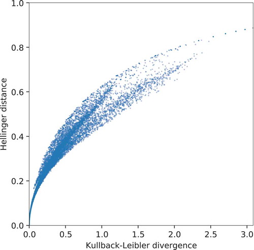
There is very little practical difference between the Hellinger distance and the Kullback-Leibler divergence in the context of this article. As can be seen in Figure 1, both measures correlate strongly in case of OSM data. For small distances, both distance measures relate almost one-to-one. Larger deviations can only be observed for medium distances. The Hellinger distance is more sensitive towards small deviations from Benford’s law, which is why we decided to focus on the Hellinger distance in the scope of this article.

Figure 1. Comparison of the Hellinger distance and the Kullback-Leibler divergence. The plot contains data for all combinations of aspects considered and all countries

4. Results

This section outlines the findings derived by using the methods explained in the Methods Section. Following these methods, many aspects of the OSM dataset have been extracted, thus yielding a chunk of data for each aspect and each country. These chunks of data, in turn, have been compared to Benford’s law. First and as a result of this comparison, thematic patterns are discussed, to then explore spatial patterns related to these thematic aspects. Finally, the effect of scale and sample size on Benford’s law is studied.

4.1. Thematic patterns

It has been demonstrated by Benford (1938) that many aspects of geographical data follow Benford’s law. Not every aspect, however, follows the law, which is why we exemplarily examine several aspects of OSM data and check which of them are in accordance with Benford’s law. As becomes visible by the vertical stripe pattern in Figure 2 (i.e., the patterns in long direction), whether Benford’s law describes the data well or not depends, for the most part, only on the aspect examined. In contrast to this, there is only little systematic variance among the different countries, which leads to less distinct horizontal patterns compared to the vertical ones, an observation discussed later on in more detail.

Figure 2. Comparison of several aspects of the OSM data to Benford’s law. High similarity (short Hellinger distance) between the actual distribution of an aspect in the OSM data and the Benford distribution is depicted in yellow, while low similarity (large Hellinger distance) is depicted in red and purple

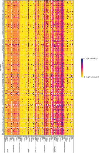
The vertical pattern correlates, with minor exceptions only, well to the numerical features. For example, the distance between the nodes defining a geometry and the length of linear features are in accordance with Benford’s law independent of the considered set of elements. The bearing defined by the first and last node of a linear feature does, however, not follow the law, which is an effect of being in the range of 0° to 360°. Even when normalizing the bearing to $0$ to $1$, the resulting values do not follow the law as every cardinal direction can be expected to appear about as often as any other one. Also, the length of tag values does not follow Benford’s law. There is one predominant tag for each set of elements because this predominant tag is presumed by the very definition of a set of elements (such as “building”=“yes” for buildings and “landuse”=“residential” for residential areas). In addition, the list of tags is often fairly short, which is why this predominant tag distorts the statistical properties of the list of tags to a high degree. Further, the number of versions does not follow the law because the great majority of elements has too few versions. In case of the elevation of peaks and the population of towns and cities, the limited availability of data has an effect on the statistical significance. This argument might be part of the explanation for why these aspects do not follow the law to the same degree, but this argument is not able to serve as an explanation alone. As becomes apparent by these examples, the vertical patterns can often be explained in terms of the ways the numerical features are defined and the resulting distribution of the corresponding values.

The nature of the numerical features cannot explain the vertical patterns alone as the same numerical feature can be very different for different sets of OSM elements. One such exception is, e.g., the number of versions in case of secondary and tertiary roads. In these cases the number of versions follows Benford’s law while it does not in other cases. The latter can be understood at the example of buildings, for which the law does not apply in general as most buildings have never been modified and thus have only one version. In overall, no difference could be detected with respect to the law in whether an aspect is part of the actual contributed data, or whether it is metadata describing the contribution. These observations provide answers to RQ1a.

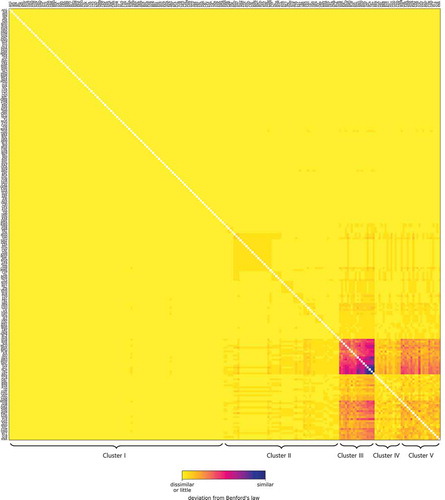
While the vertical patterns are very distinctive, the values in the matrix of Figure 2 expose statistical variance. Figure 3 explores how similar this statistical variance is within a pair of columns of the matrix. For each pair of aspects, it is counted for how many countries these two aspects do coincidentally not follow Benford’s law. As such a comparison is of particular relevance for aspects that generally follow the law, only those aspects with a Hellinger distance larger than $0.1$ for at least 80% of the countries have been considered. In order to study the clusters formed by aspects with similar spatial patterns, the rows and columns have been reordered likewise. To achieve such clusters, the rows and columns have, first, been clustered hierarchically using the Ward variance minimization algorithm (Ward 1963). Then, these hierarchical clusters have been flattened to a cophenetic distance of half of the maximal distance. For each of these resulting clusters, the clustering was repeated recursively. As a result, the matrix exposes a block form, describing how the statistical variance of several aspects clusters.

Figure 3. Similarity of spatial patterns for pairs of aspects. Each cell encodes the number of countries for which these two aspects do coincidentally not follow Benford’s law, i.e., for which the Hellinger distance between the actual distribution and the Benford distribution is larger than $0.1$. Only aspects for which at least 80% of the countries follow the law have been included. The rows and columns have been reordered in order to achieve a block form

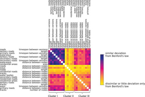
In the matrix of Figure 3, three clusters can be distinguished. The aspects of Cluster I are mutually strongly similar by the fact that there are many countries in which Benford’s law does coincidentally not apply to neither of the considered aspects. This is in contrast to the Clusters II and III, the aspects of which expose no or only much weaker mutual similarity. Remarkably, the aspects from Clusters I and III are more similar than the aspects of Clusters III mutually are. This demonstrates that there exists a predominant pattern in the way Benford’s law applies to an aspect of OSM data. The assignment of the aspects to the clusters does not seem to follow any obvious pattern. These observations provide answers to RQ1b.

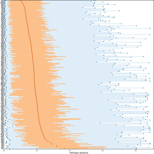
Figure 4 explores again the heterogeneity that can be found in the matrix of Figure 2. In contrast to Figure 3, which explores the similarity of pairs of columns in this matrix, Figure 4 depicts information about the heterogeneity per column. That is, it shows the median and the the 25%–75%-quantile of the Hellinger distance between the distribution in the actual data (country level) and the Benford distribution for each of the aspects. This way, the heterogeneity of the Hellinger distance across the countries can be visually assessed.

Figure 4. Spatial heterogeneity of the Hellinger distance for several aspects. For every aspect, the lowest and highest Hellinger distance observed are depicted in dark blue. The 25%–75%-quantile is depicted in bright orange, and the median is depicted in dark orange

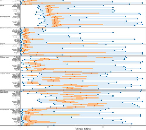
The heterogeneity of Hellinger distances varies across numerical features. As is apparent by Figure 4, the minimum, median, and maximum of the Hellinger distances vary considerably across the various aspects. This is despite the fact that for most aspects, there exist countries in which the data do not follow the law, even if the median is very low and the aspect can be considered to follow Benford’s law in general. There are only very few exceptions, such as the distance between the nodes in case of primary roads, residential areas, residential roads, and roads in general. In these cases, even the maximum value is relatively low. Besides the minima, medians, and maxima themselves, also their heterogeneity strongly depends on the numerical feature considered. The minima expose, e.g., very little heterogeneity in case of the distance between nodes and the length of linear features, while exposing high heterogeneity in case of the number of nodes, the number of versions, and the tag value length. In general, the heterogeneity of the minima and medians is much higher in cases where the average distance between the actual distribution and the Benford distribution is larger. In case of high average similarity, i.e., small distance of the actual distribution to the Benford distribution, the heterogeneity of the minima and medians is much lower, indicating that Benford’s law is relatively stable across different sets of OSM elements for the same numerical feature. These observations provides answers to RQ1c.

4.2. Spatial patterns related to thematic aspects

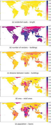
The degree to which OSM data follow Benford’s law exposes spatial patterns. In this section, we examine the global spatial patterns in more detail. Figure 5 shows the Hellinger distance to the Benford distribution, thereby illustrating whether neighbouring countries follow Benford’s law in the same way. In some cases, there is little variance in the Hellinger distance to the Benford distribution across the countries, as is the case for the length of residential roads (Figure 5a) and the number of versions of buildings (Figure 5b). In particular in the case of Figure 5a, no significant spatial patterns can be observed. In other cases, the similarity is spatially less homogeneously distributed (Figure 5c–e). That is, there exist strong spatial patterns in the heterogeneity of the similarity values. In particular, countries in Africa and to a lesser degree also in South America expose a much higher heterogeneity for single aspects than countries on other continents. This observation applies across multiple aspects, and it applies to some countries outside Africa too, e.g., to Greenland, India, Afghanistan, Papua New Guinea, and Mongolia. One possible explanation is the low number of OSM elements available for African countries³ and, in parts related to these low numbers, the mixed data quality. In case of the completeness of the road network, Barrington-Leigh and Millard-Ball (2017) have observed the same heterogeneity among African countries. However, it might be suspected that there are more reasons besides this fact for why Africa is different in the discussed context. These observations about the regimes, in particular with respect to the heterogeneity, answer RQ2a.

Figure 5. Areal maps depicting the degree to which Benford’s law applies to OSM data of different regions. The maps indicate the Hellinger distance between the OSM data and the Benford distribution by the colour scheme used. The country borders have been extracted from OSM data, thus including maritime boundaries in parts, and they have been generalized. The maps use the Behrmann projection

An approach similar to the one used for Figure 3 can be utilized to examine the similarity between countries in terms of how well their aspects follow Benford’s law. In Figure 6, it is explored how similar this statistical variance is within two rows of the matrix presented in Figure 2. Again and very similar to the situation in Figure 3, several clusters can be identified. Cluster III contains countries the data of which in any cases coincidentally do not follow Benford’s law. That is, these countries have a high number of aspects in common that do not follow Benford’s law. Among these are many island countries (such as the British Virgin Islands, Kiribati, Palau, Niue, South Georgia and the South Sandwich Islands, the Maldives, the Marshall Islands, Tuvalu, and Pitcairn); other very small countries (such as Monaco and Vatican City); and Antarctica as a very sparsely populated area. Cluster V shows the same behaviour as Cluster III but to a much lesser degree: many aspects of the countries of Cluster V coincidentally do not follow Benford’s law. The countries of the Clusters III and V, however, are even more similar with respect to their aspects’ behaviour as the countries of Cluster V are mutually. Again, Cluster V is composed by many island countries (such as the Federated States of Micronesia, Dominica, the Cook Islands, Tonga, Falk Islands, Guernsey, and the Solomon Islands); other small countries (such as Gibraltar, San Marino, and Andorra); and Kuwait. Cluster II and IV contain countries the data of which are only very slightly similar in the described sense, but even more sporadically in case of Cluster II. These clusters are formed by a larger diversity of countries: among others, by African countries (such as Congo, Guyana, Suriname, Gambia, Senegal, Libya, and Morocco); further countries from the Global South (such as Bhutan, Qatar, Brunei, and Colombia); sparsely populated countries (Greenland); island countries (such as Barbados, Saint Lucia, and Bahamas); the USA; and some few European countries (such as the Netherlands, Norway, and Estonia). The countries of Cluster I – countries from all over the world, including most European countries and countries being very large in extent (such as Australia, Russia, Brazil, and China) – expose almost without exception no such similarity. This answers RQ2b.

Figure 6. Similarity of thematic patterns for pairs of countries. Each cell encodes the number of aspects for which the corresponding two countries do coincidentally not follow Benford’s law, i.e., for which the Hellinger distance between the actual distribution and the Benford distribution is larger than $0.1$. Only countries for which at least 80% of the aspects follow the law have been included. The rows and columns have been reordered in order to achieve a block form

While spatial differences exist in the ways Benford’s law applies to country-specific data for single aspects (Figure 5), little variation can be observed when considering all aspects simultaneously (Figure 7). Data related to most of the countries show similar characteristics. The heterogeneity of both the 25% and the 75%-quantile slightly increases for higher medians, while the overall minimum and maximum with respect to the Hellinger distance are almost stable, which answers RQ2c. At the lower end of the diagram (larger Hellinger distance), island countries can be found (such as Tokelau, the Marshall Islands, Pitcairn, and the British Indian Ocean Territory). The countries Norway, Austria, and Sweden appear at the upper end, actually before the global Hellinger distance. In other words, the data in these countries is better described by Benford’s law than the global dataset, indicating that some processes underlying the data can have more influence on the Hellinger distance than the size of the statistical population. This, in turn, indicates that Benford’s law is a meaningful description of at least some processes generating the data.

Figure 7. Spatial heterogeneity of the Hellinger distance, aggregated for all aspects. For every aspect, the lowest and highest Hellinger distance observed are depicted in dark blue. The 25%–75%-quantile is depicted in bright orange, and the median is depicted in dark orange

4.3. The effect of scale and sample size

Benford’s law is of statistical nature. This is why it tends to apply less well in case of small sample size. As has been seen before, Benford’s law tends to describe OSM data worse in case of small island countries and much better in case of larger countries with good OSM coverage, both in terms of the absolute Hellinger distance as well as in terms of the corresponding heterogeneity. In contrast to the examination of the data on a more global scale in previous sections, the effect of the sample size and of spatially local phenomena on whether the law applies is examined in this section.

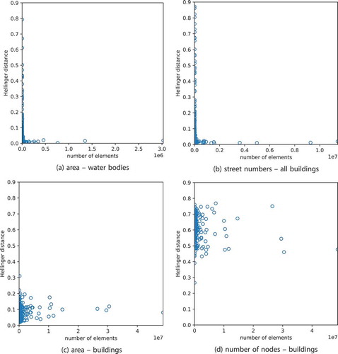
Figure 8 examines the influence of the sample size, i.e., of the number of elements considered, on the Hellinger distance. It can be expected that Benford’s law applies to a lesser degree to small sets of numbers, i.e., a small set of OSM elements, and that it applies to a higher degree to larger sets. It turns out that this expectation is, by and large, true for those aspects for which the data follow the law at least for most countries at larger spatial scales. This applies, e.g., to the area of water bodies and the street numbers of all buildings (Figure 8a–b). If the number of elements is large, the data follows Benford’s law, while for countries with a smaller set of OSM elements, it does so to a lesser and varying degree. The distributions of the points in the scatter plots thus follow an L-shaped distribution. In other cases in which Benford’s law does not apply at all, no L-shaped distribution can be observed. Instead, the Hellinger distance is to a high degree independent of the number of elements. This applies, e.g., to the number of nodes of buildings (Figure 8d). If the data, however, expose a distribution that is only slightly similar to the Benford distribution – in some sense, the data can be considered to be between the two extremes discussed before in this case – the similarity to the Benford distribution tends to converge in many cases towards a certain fixed value for an increasing number of elements. This is, e.g., the case for the area of buildings (Figure 8c). These observations answer RQ3a.

Figure 8. Correlation between the number of elements considered (sample size) and the Hellinger distance

Note that the x-axes are scaled differently.

In many cases, the area examined is of relevance, and not the number of elements. This is, e.g., the case when assessing the quality of OSM data in a given area. Figure 9 thus examines the influence of the study area on the Hellinger distance. Different near-quadratic study areas have been considered, each of them being of different size and centred around one of three exemplary locations: The Museum of Modern Art, also known as MoMA, New York City, NY, USA; the Eiffel Tower, Paris, France; and the Faculty of Geo-Information Science and Earth Observation (ITC), University of Twente, Enschede, the Netherlands. Thereby, the study area is varied systematically from 222 km down to about 2 m.

Figure 9. Influence of the study area on the Hellinger distance. No curve is drawn if no relevant data is contained in the study area. Note that the x-axes are scaled differently

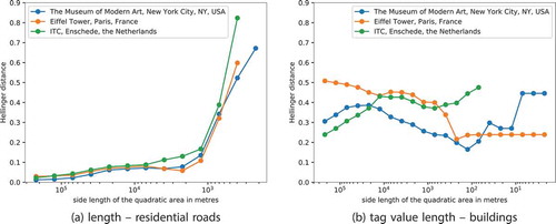
As can be expected, the size of the study area has an effect on how well the data follow Benford’s law. For many aspects of the OSM dataset, the law applies for smaller cartographic scales while it does not apply for larger scales. The example of the length of residential roads shows that the actual distribution of leading digits is very similar to the Benford distribution for scales of analysis down to about 2 km, and it significantly increases below (Figure 9a). Also, there is very little variation with respect to the three centre points, even though these are in different geographical contexts and the population density strongly differs among the considered cities. In most cases, the Hellinger distance is stable down to a certain threshold. However, in cases in which Benford’s law does not apply the scale dependency is more chaotic. This is, e.g., the case for the tag value length of buildings (Figure 9b). The very different behaviour related to the scale dependency among the considered locations cannot be explained in the same systematic way as is the case in the previous example. These observations answer RQ3b.

5. Discussion

The universality of Benford’s law is astonishing. There is no formal reason for why the law should apply to many types of data, and why it should apply to geographical data in particular. Despite that, the distribution of leading digits is for many aspects very similar to the Benford distribution, as has been shown before and explored for a larger number of aspects of geographical data in this article. While some of the aspects examined are specific to OSM, such as the length of tag values or the number of versions, many conclusions of generic character can be drawn. As an example, whether the data follow Benford’s law strongly depends on the aspect displayed but much less on the geographical region (Figures 2 and 4). This observation suggests that the patterns are largely independent of OSM. They rather depend on the particular aspect considered. It has turned out that some aspects of the data are very similar both in terms of in which countries they follow Benford’s law (Figures 2 and 5) and in the spatial heterogeneity they expose with respect to the Hellinger distance (Figure 4). There is little reason to believe that this pattern of similarities among the aspects would be restricted to OSM only. Quite to the contrary, the cluster of aspects emerging after reordering is very distinctive and does not refer to a specific characteristic of the data only (Figure 3). It can thus be expected that similar clusters also exist for other datasets and other choices of aspects. Also, there is little spatial heterogeneity in case of those aspects in which the data follow Benford’s law (Figure 4). This observation seems to be of more universal character too. The patterns of where the data deviate from Benford’s law are, in case of OSM, partly spatial in nature, partly related to the size of the examined area (Figure 5,6 and 7). The spatial patterns often relate to areas in which data quality might be worse and to areas of smaller size, in particular, to island countries and very small countries. The same reasons for spatial patterns in the deviation from the law can be assumed for similar datasets because these reasons are of rather universal nature, suggesting that the conclusions drawn are valid even beyond OSM data.

The results derived provide insights about the limitations of Benford’s law in the context of OSM data. Due to the statistical nature of Benford’s law, it can be expected that the smaller the sample size (or, the study area), the more deviates the distribution found in the data from the distribution predicted by Benford’s law. We have investigated this dependency and have shown that, in many cases, the effect of a small study area disturbs the statistical patterns related to the traceability of Benford’s law in OSM data first when examining an area of 2 km in diameter or below (Figure 9). This effect poses limitations to the prediction power related to the law.

In contrast to many previous studies that do not target the spatial context of Benford’s law (e.g., Benford 1938, Deckert et al. 2011, Rauch et al. 2011), we have shown that spatial patterns exist in the way OSM data follow the law. As an example, we have identified African countries to expose particularly high level of heterogeneity. This demonstrates that Benford’s law is able to capture at least some aspects that are of importance in a spatial context. Despite the fact that this high level of heterogeneity is straightforward to trace in the data, good explanations are rare. Data quality alone seems not to be a complete answer to this question.

6. Future prospects and limitations in the context of data quality assessment

One way to uncover bad data quality or irregularities in the data is to compare the meaning of the data to rules, patterns, or general knowledge (Mocnik et al. 2018). Data often expose patterns that hold true in general but are breached in case of bad quality or irregularities. When such patterns are used to identify potential cases of bad data quality, large amounts of data can be screened automatically. Only the suspicious parts of the data need to be examined manually and in more detail. Benford’s law is used in the context of economic and other datasets as such a pattern. Deviation from the law is used to detect indications for fraud in such datasets: if the data deviates from Benford’s law although it could generally be expected that this law applies, this indicates that the data might be created by fraudulent activities. The same might be possible for geographical data in general and OSM data in particular: if some aspect of the data deviates from Benford’s law for a particular area despite being in accordance with the law in general, this might indicate data quality issues.

We have explored how well Benford’s law applies to OSM data with respect to numerical aspects, several sets of elements, spatial variations, and further aspects in Sections 3–5. While we were able to show that Benford’s law applies in many cases, this does not yet yield any data quality indicator. As has been outlined in the introduction, the question for which data quality issues and irregularities Benford’s law is violated needs to be addressed. Combining the knowledge about these issues and irregularities and about the way Benford’s law applies to OSM data in general may lead to easy-to-use indicators in the future.

Obviously, wrong data or data of bad quality cannot per se be detected using Benford’s law. If someone deliberately contributes data that contradict reality (such as a house next to a road at a place where there is no house) in a way similar to other contributions, this cannot be expected to be detected by any intrinsic approach. The same applies to contributions that seem to be illogical in the geographical context but comply otherwise with the pattern found in the data. What can potentially be detected are structures imposed by processes that are usually not expected to play a role in the contribution context of OSM data. In the context of economic data, for instance, fraud or manipulation in a more general sense can often be detected because corresponding data are created manually and not by economic processes. Accordingly, the distribution of the numbers and their leading digits is, in this case, not any longer determined by economic processes and how these scale but by what the person who creates the data intuitively thinks makes sense.

In the following, three examples of irregularities and potential causes for data quality issues are outlined in the context of OSM and Benford’s law.

Example 1: Bots. In contrast to humans, bots contribute to OSM in a more mechanistic way, often leading to a more regular temporal scheme and a more systematic way of using tags. These patterns can be expected to be detectable. On the one hand, we have shown that for most sets of elements, the timespan between two versions follows Benford’s law. On the other hand, if a bot reacts to a contribution by adding a tag or modifying the geometries, this often happens with a near-to-constant temporal delay to the corresponding contribution the bot reacts to. Other bots search the data at regular intervals, which limits the temporal delay between the original distribution and the modification by the bot too. Accordingly, it can be expected that temporal patterns related to the contribution by bots are different to the ones by humans and accordingly might fail to follow Benford’s law in many cases.

Example 2: Vandalism. Some contributions aim to deliberately decrease data quality. Such vandalism can be very different in nature. For some types of vandalism, there is a high chance that it goes unnoticed if the contribution could represent an existing geographical feature and if it follows the same patterns as any other contribution. This is, however, often not the case. Many cases of vandalism differ from other contributions, for instance, in the spatial patterns occurring or the random modification and deletion of objects, which are potentially distributed across a wide area (Neis et al. 2012, Truong et al. 2018). A detailed examination of cases of vandalism will show which aspects of the data are suitable to uncover which type of vandalism best.

Example 3: Data imports. Parts of the OSM dataset are the result of importing other datasets. Such imports are not necessarily a sign of bad data quality. If the data imported are of high quality and show little heterogeneity in this aspect, the data quality of OSM can even improve. The import of TIGER/Line data in the US, for instance, has initially improved the completeness of the OSM dataset. However, it often happens that the categories used for the classification of geographical features are not coherently used in the imported dataset and the dataset imported to, which, in turn, can create semantic data quality issues. Also, data imports can have positive or negative impact on the correction of the coordinates to compensate for tectonic plate motion (Mocnik 2021). In either way, a data import can have an impact on the data quality of the dataset the import is incorporated in. Data imports lead to a distortion of the contribution timeline because the representations of many geographical features in the OSM dataset are added or modified at virtually the same point in time. Further, the orientation of the geographical features imported might be biased and the spatial accuracy of the representation different, compared to those representations already existing in the OSM dataset. Further, the distance between nodes, the minimal area of the contributed features, the number of nodes per feature, and so on can be different for the imported dataset and the dataset imported to. Not all of these aspects follow Benford’s law, which is why it is necessary to check in more detail which aspects are suitable to uncover potentially unnoticed data imports and corresponding effects on data quality.

If Benford’s law does not apply to a set of elements, either defined by their spatial extent, the timeframe in which the data were contributed, or some other thematic context, this can only indicate suspicious contributions. What is and remains necessary is to check cases of suspicious contributions by hand, a fact that, indeed, applies to every intrinsic measure (cf., Mocnik et al. 2018). Such checking presumes geographical expertise and careful consideration of the results provided by the comparison to Benford’s law.

This study at hand demonstrates that some aspects of the OSM data follow Benford’s law while others do not. This result suggests that there is no general rule to which numerical features, geographical entities, and spatial regions Benford’s law applies. However and despite this lack of generality, we have demonstrated that certain numerical features follow Benford’s law for several geographical entities and in many regions. This suggests that Benford’s law also applies to similar datasets. In order to utilize Benford’s law with respect to data quality assessment, more specific examples of irregularities and potential causes for data quality issues including the ones outlined above need to be studied in the next step. We have in this article identified the need to study corresponding aspects in more detail and on an individual level. At the same time, the results suggest that such specialized studies will be able to successfully reveal those aspects that are in accordance with Benford’s law. In addition to specialized studies and when having sufficient data quality information at hand, the correlations between various data quality measures and the deviation of the data from Benford’s law could be explored more systematically, e.g., by using a formal framework as has been proposed by Mocnik (2018a).

Intrinsic laws, such as Benford’s law, are limited by their intrinsic way of identifying issues in the data and thus their potential use for improving the quality of the data. As there exist many alternative ways of assessing data quality, as is suggested by data quality ontologies (Wand and Wang 1996, Frank 2007, Goodchild and Li 2012, Mocnik et al. 2018), it seems logical to explore the additional benefits of using Benford’s law in combination with other approaches. For instance, parts of the data that turn out not to follow Benford’s law might be compared to local knowledge (Poiani et al. 2016, Klonner et al. 2018). Future research might discuss how such different methods can be tightly integrated to improve the quality of the actual assessment as well as corresponding actions to improve the data.

Besides the question of the aspects to which Benford’s law applies, this study has explored the limitations of Benford’s law in the context of OSM data on both local and global scales. Referring to the former, the effect of the size of the study area and the sample size on Benford’s law has been explored. The results suggest that a meaningful detection of irregularities can only happen at neighbourhood or town scale and at corresponding sample sizes. While this limits the applicability of the discussed approach in case of small-scale scenarios, intrinsic data quality indicators are often created with the aim of monitoring large volumes of data. Referring to the global scale, we have shown that the Hellinger distance between the OSM data and the Benford distribution exposes spatial patterns and is far from being homogeneous. It seems logical to explore whether corresponding more local spatial patterns exist as well, for instance, by using corresponding statistical means related to the detection of spatially structured variance (Westerholt et al. 2018). The in-depth investigation of actual examples of irregularities in general can be expected to reveal further limitations, both with respect to the OSM as well as other geographical datasets.

7. Conclusions and future work

Benford’s law makes possible to uncover global and regional spatial patterns. Future research might focus on a better understanding of the reasons behind these spatial patterns. Data quality might be part of the explanations but our current knowledge about the reasons behind these spatial patterns is yet limited. It is thus subject to future research to explore what constitutes these spatial patterns, and why Benford’s law is able to make these patterns visible. In particular, these patterns might not directly be related to Benford’s law, but they are at least traceable through utilizing the law.

Related to tracing spatial patterns, future research might explore in more detail in which ways the law is applicable to spatial areas, and what the resulting similarity of the distribution in the data to the Benford distribution is able to uncover about the data. In this article, we have shown that there is a minimum study area (depending on the aspect considered) when comparing the data to Benford’s law in a meaningful way. Beyond that, different sizes of study areas imply different scales of analysis. It is yet unclear which size of an area and which corresponding scale of analysis is able to detect which type of phenomenon, and whether the observed deviation from the law with respect to certain aspects and certain countries is the result of detected data quality issues, or whether other factors are the reason for these limitations. Which size of the study area is, e.g., able to uncover mapping events by examining the point in time of the contributions? How must the scale of analysis systematically be varied in order to detect data imports? Can vandalism in OSM be detected by the patterns it imposes? Are we able to detect so far unknown effects related to OSM or VGI in general?

This article has identified some connections between Benford’s law and data quality assessment in the case of OSM and explored its future prospects and limitations. As future research, several examples of irregularities, vandalism, imports, and bad data quality need to be examined in more detail. If it turns out that some aspects of these examples do not follow the Benford distribution while the same aspects do in general, this would provide a potential indicator for data quality related issues.

Only few laws have been discussed in the context of geographical or spatial information. Tobler’s first and second law of Geography are two of the few exceptions. In contrast to Tobler’s laws, Benford’s law did (so far) not receive much attention with respect to geographical information. In this sense, studying the law in the context of geographical information in more detailed ways and for further datasets is a logical next step towards future uses of Benford’s law.

Data and codes availability statement

The OpenStreetMap dataset can be downloaded at https://planet.openstreetmap.org. The data has been processed by the OSHDB software (Raifer et al., 2019). The corresponding code and further figures have been made available at https://doi.org/10.6084/m9.figshare.12991499.v1.

Disclosure statement

No potential conflict of interest was reported by the author.

Additional information

Funding

This work has partly been supported by the Heidelberg Academy of Sciences and Humanities project Heterogeneity and convergence in shared data sources – the importance of cognitive coherence in collective decision making.

Notes on contributors

Franz-Benjamin Mocnik

Franz-Benjamin Mocnik is an Assistant Professor at the University of Twente, where he conducts research about structural aspects in Geographical Information Science, such as laws and patterns, as well as about platial information. He received a doctoral degree from the Vienna University of Technology in the field of Geographical Information Science and holds a Diplom degree in the field of Mathematics. As a postdoctoral fellow, he worked at Heidelberg University and was a twin fellow of the Hanse-Wissenschaftskolleg, Institute for Advanced Study.  For his work, he was awarded the Waldo-Tobler Young Researcher Award.

Notes

1. The notion of Geographical Shared Data Sources has been adapted from a publication by Mocnik et al. (2019).

2. Compare https://resultmaps.neis-one.org

3. Currently, only 10.5% of the nodes, 11.2% of the ways, and 2.2% of the relations in OSM are about Africa. In comparison, about 17% of the world’s population lives in Africa, and Africa accounts for about 20% of all landmasses.

References

- Barrington-Leigh, C. and Millard-Ball, A., 2017. The world’s user-generated road map is more than 80% complete. PLoS ONE, 12 (8), e0180698. doi:10.1371/journal.pone.0180698.
- Benford, F., 1938. The law of anomalous numbers. Proceedings of the American Philosophical Society, 78 (4), 551–572.
- Berger, A. and Hill, T.P., 2011a. A basic theory of Benford’s law. Probability Surveys, 8, 1–126. doi:10.1214/11-PS175.
- Berger, A. and Hill, T.P., 2011b. Benford’s law strikes back: no simple explanation in sight for mathematical gem. The Mathematical Intelligencer, 33 (1), 85–91. doi:10.1007/s00283-010-9182-3.
- Bjorholm, S., et al. 2008. To what extent does Tobler’s 1st law of geography apply to macroecology? A case study using American plams (Aracaceae). BMC Ecology, 8 (11). doi:10.1186/1472-6785-8-11.
- Crocetti, E. and Randi, G., 2016. Using the Benford’s law as a first step to assess the quality of cancer registry data. Frontiers in Public Health, 4, 225. doi:10.3389/fpubh.2016.00225.
- Deckert, J., Myagkov, M., and Ordeshook, P.C., 2011. Benford’s law and the detection of election fraud. Political Analysis, 19 (3), 245–268. doi:10.1093/pan/mpr014.
- Durtschi, C., Hillison, W., and Pacini, C., 2004. The effective use of Benford’s law to assist in detecting fraud in accounting data. Journal of Forensic Accounting, 5, 11–34.
- Fewster, R.M., 2009. A simple explanation of Benford’s law. The American Statistician, 63 (1), 26–32. doi:10.1198/tast.2009.0005.
- Formann, A.K., 2010. The Newcomb–Benford law in its relation to some common distributions. PLoS ONE, 5 (5), e10541. doi:10.1371/journal.pone.0010541.
- Frank, A.U., 2007. Data quality ontology: an ontology for imperfect knowledge. Proceedings of the 8th Conference on Spatial Information Theory (COSIT), 406–420. Melbourne, Australia. doi:10.1007/978-3-540-74788-8_25.
- Furry, W.H. and Hurwitz, H., 1945. Distribution of numbers and distribution of significant figures. Nature, 155, 52–53. doi:10.1038/155052a0.
- Gauvrit, N. and Delahaye, J.-P., 2009. Loi de Benford générale. Mathématiques et sciences humaines, 186, 5–15. doi:10.4000/msh.11034.
- Geyer, A. and Martí, J., 2012. Applying Benford’s law to volcanology. Geology, 40 (4), 327–330. doi:10.1130/G32787.1.
- Goodchild, M.F. and Li, L., 2012. Assuring the quality of volunteered geographic information. Spatial Statistics, 1, 110–120. doi:10.1016/j.spasta.2012.03.002.
- Goudsmit, S.A. and Furry, W.H., 1944. Significant figures of numbers in statistical tables. Nature, 154, 800–801. doi:10.1038/154800a0.
- Haklay, M., 2010. How good is volunteered geographical information? A comparative study of Open- StreetMap and Ordnance Survey datasets. Environment and Planning B, 37 (4), 682–703. doi:10.1068/b35097.
- Hecht, B. and Moxley, E., 2009. Terabytes of Tobler: evaluating the first law in a massive, domain-neutral representation of world knowledge. Proceedings of the 9th Conference on Spatial Information Theory (COSIT), 88–105. Aber Wrac'h, France. doi:10.1007/978-3-642-03832-7_6.
- Hellinger, E., 1909. Neue Begründung der Theorie quadratischer Formen von unendlichvielen Veränderlichen. Journal für die reine und angewandte Mathematik, 136, 210–271. doi:10.1515/crll.1909.136.210.
- Hill, T.P., 1995a. Base-invariance implies Benford’s law. Proceedings of the American Mathematical Society, 123 (3), 887–895.
- Hill, T.P., 1995b. A statistical derivation of the significant-digit law. Statistical Science, 10 (4), 354–363. doi:10.1214/ss/1177009869.
- Jolion, J.-M., 2001. Images and Benford’s law. Journal of Mathematical Imaging and Vision, 14 (1), 73–81. doi:10.1023/A:1008363415314.
- Judge, G. and Schechter, L., 2009. Detecting problems in survey data using Benford’s law. The Journal of Human Resources, 44 (1), 1–24. doi:10.3368/jhr.44.1.1.
- Klonner, C., et al. 2018. Capturing flood risk perception via sketch maps. ISPRS International Journal of Geo-Information, 7 (9), 359. doi:10.3390/ijgi7090359.
- Kullback, S. and Leibler, R., 1951. On information and sufficiency. The Annals of Mathematical Statistics, 22 (1), 79–86. doi:10.1214/aoms/1177729694.
- Mayer, M., Heck, D.W., and Mocnik, F.-B., 2020. Shared mental models as a psychological explanation for converging mental representations of place – the example of OpenStreetMap. Proceedings of the 2nd International Symposium on Platial Information Science (PLATIAL’19), 43–50. Coventry, UK. doi:10.5281/zenodo.3628871.
- Miller, H.J., 2004. Tobler’s first law and spatial analysis. Annals of the Association of American Geographers, 94 (2), 284–289. doi:10.1111/j.1467-8306.2004.09402005.x.
- Mir, T.A., Ausloos, M., and Cerqueti, R., 2014. Benford’s law predicted digit distribution of aggregated income taxes: the surprising conformity of Italian cities and regions. The European Physical Journal B, 87, 261. doi:10.1140/epjb/e2014-50525-2.
- Mocnik, F.-B., et al., 2018. A grounding-based ontology of data quality measures. Journal of Spatial Information Science, 16, 1–25. doi:10.5311/JOSIS.2018.16.360.
- Mocnik, F.-B., 2018a. Linked open data vocabularies for semantically annotated repositories of data quality measures. Proceedings of the 10th International Conference on Geographic Information Science (Giscience), 50:1–50:7. Melbourne, Australia. doi:10.4230/LIPIcs.GISCIENCE.2018.50.
- Mocnik, F.-B., 2018b. The polynomial volume law of complex networks in the context of local and global optimization. Scientific Reports, 8, 11274. doi:10.1038/s41598-018-29131-0.
- Mocnik, F.-B., et al. 2019. Shared data sources in the geographical domain—a classification schema and corresponding visualization techniques. ISPRS International Journal of Geo-Information, 8 (5), 242. doi:10.3390/ijgi8050242.
- Mocnik, F.-B., Westerholt, R. 2021. The effect of tectonic plate motion on georeferenced long-term global datasets. International Journal of Applied Earth Observation and Geoinformation, 94, 102183. doi:10.1016/j.jag.2020.102183.
- Mocnik, F.-B. and Frank, A.U., 2015. Modelling spatial structures. Proceedings of the 12th Conference on Spatial Information Theory (COSIT), 44–64. Santa Fe, NM, USA. doi:10.1007/978-3-319-23374-1_3.
- Mocnik, F.-B., Zipf, A., and Raifer, M., 2017. The OpenStreetMap folksonomy and its evolution. Geo- Spatial Information Science, 20 (3), 219–230. doi:10.1080/10095020.2017.1368193.
- Neis, P., Goetz, M., and Zipf, A., 2012. Towards automatic vandalism detection in OpenStreetMap. ISPRS International Journal of Geo-Information, 1 (3), 315–332. doi:10.3390/ijgi1030315.
- Newcomb, S., 1881. Note on the frequency of use of the different digits in natural numbers. American Journal of Mathematics, 4 (1), 39–40. doi:10.2307/2369148.
- Nigrini, M.J., 1996. A taxpayer compliance application of Benford’s law. The Journal of the American Taxation Association, 18 (1), 72–91.
- Nigrini, M.J. and Wells, J.T., 2012. Benford’s law. Applications for forensic accounting, auditing, and fraud detection. Hoboken, NY: Wiley. doi:10.1002/9781119203094.
- Niskanen, J. and Keloharju, M., 2000. Earnings cosmetics in a tax-driven accounting environment: evidence from Finnish public firms. European Accounting Review, 9 (3), 443–452. doi:10.1080/09638180020017159.
- Pérez-González, F., Heileman, G.L., and Abdallah, C.T., 2007. Benford’s law in image processing. Pro- ceedings of the 14th IEEE International Conference on Image Processing, 405–408. San Antonio, TX, USA. doi:10.1109/ICIP.2007.4378977.
- Pinkham, R.S., 1961. On the distribution of first significant digits. The Annals of Mathematical Statistics, 32 (4), 1223–1230. doi:10.1214/aoms/1177704862.
- Poiani, T.H., et al., 2016. Potential of collaborative mapping for disaster relief: a case study of Open- StreetMap in the Nepal earthquake 2015. Proceedings of th 49th Hawaii International Conference on System Sciences, 188–197. Koloa, HI, USA. doi:10.1109/HICSS.2016.31.
- Raifer, M., et al., 2019. OSHDB: a framework for spatio-temporal analysis of OpenStreetMap history data. Open Geospatial Data, Software and Standards, 4 (3). doi:10.1186/s40965-019-0061-3.
- Raimi, R.A., 1976. The first digit problem. The American Mathematical Monthly, 83 (7), 521–538. doi:10.1080/00029890.1976.11994162.
- Raimi, R.A., 1985. The first digit problem again. Proceedings of the American Philosophical Society, 129 (2), 211–219.
- Rauch, B., et al. 2011. Fact and fiction in EU-governmental economic data. German Economic Review, 12 (3), 243–255. doi:10.1111/j.1468-0475.2011.00542.x.
- Sandron, F., 2004. Les populations suivent-elles la loi des nombres anomaux? Population, 57, 753–761. doi:10.3917/pope.204.0753.
- Shi, J., Ausloos, M., and Zhu, T., 2018. Benford’s law first significant digit and distribution distances for testing the reliability of financial reports in developing countries. Physica A, 492, 878–888. doi:10.1016/j.physa.2017.11.017.
- Skousen, C.J., Guan, L., and Wetzel, T.S., 2004. Anomalies and unusual patterns in reported earnings: Japanese managers round earnings. Journal of International Financial Management and Accounting, 15 (3), 212–234. doi:10.1111/j.1467-646X.2004.00108.x.
- Sottili, G., et al. 2012. Benford’s law in time series analysis of seismic clusters. Mathematical Geosciences, 44 (5), 619–634. doi:10.1007/s11004-012-9398-1.
- Sui, D.Z., 2004. Tobler’s first law of geography: a big idea for a small world? Annals of the Association of American Geographers, 94 (2), 269–277. doi:10.1111/j.1467-8306.2004.09402003.x.
- Thomas, J.K., 1989. Unusual patterns in reported earnings. The Accounting Review, 64 (4), 773–787.
- Tobler, W.R., 1970. A computer movie simulating urban growth in the Detroit region. Economic Geography, 46, 234–240. doi:10.2307/143141.
- Tobler, W.R., 2004. On the first law of geography: a reply. Annals of the Association of American Geographers, 94 (2), 304–310. doi:10.1111/j.1467-8306.2004.09402009.x.
- Truong, Q.T., Touya, G., and de Runz, C., 2018. Towards vandalism detection in OpenStreetMap through a data driven approach. Proceedings of the 10th International Conference on Geographic Information Science (GIScience), 61:1–61:7. Melbourne, Australia. doi:10.4230/LIPIcs.GIScience.2018.61.
- Wand, Y. and Wang, R.Y., 1996. Anchoring data quality dimensions in ontological foundations. Communications of the ACM, 39 (11), 86–95. doi:10.1145/240455.240479.
- Ward, J.H., Jr, 1963. Hierarchical grouping to optimize an objective function. Journal of the American Statistical Association, 58 (301), 236–244. doi:10.1080/01621459.1963.10500845.
- Watrin, C., Struffert, R., and Ullmann, R., 2008. Benford’s law: an instrument for selecting tax audit targets? Review of Managerial Science, 2, 219–237. doi:10.1007/s11846-008-0019-9.
- Westerholt, R., et al. 2018. A statistical test on the local effects of spatially structured variance. International Journal of Geographical Information Science, 32 (3), 571–600. doi:10.1080/13658816.2017.1402914.
- Westlund, H., 2013. A brief history of time, space, and growth: Waldow Tobler’s first law of geography revisited. The Annals of Regional Science, 51 (3), 917–924. doi:10.1007/s00168-013-0571-3.
- Zaharis, A., et al. 2011. Lightweight steganalysis based on image reconstruction and lead digit distribution analysis. International Journal of Digital Crime and Forensics, 3 (4), 29–41. doi:10.4018/jdcf.2011100103.