Quantifying historical landscape change with repeat photography: an accuracy assessment of geospatial data obtained through monoplotting

ABSTRACT

Traditional landscape photographs reaching back until the second half of the nineteenth century represent a valuable image source for the study of long-term landscape change. Due to the oblique perspective and the lack of geographical reference, landscape photographs are hardly used for quantitative research. In this study, oblique landscape photographs from the Norwegian landscape monitoring program are georeferenced using the WSL Monoplotting Tool with the aim of evaluating the accuracy of point and polygon features. In addition, the study shows how the resolution of the chosen digital terrain model and other factors affect accuracy. Points mapped on the landscape photograph had a mean displacement of 1.52 m from their location on a corresponding aerial photograph, while mapped areas deviated on average 5.6% in size. The resolution of the DTM, the placement of GCPs and the angle of incidence were identified as relevant factors to achieve accurate geospatial data. An example on forest expansion at the abandoned mountain farm Flysetra in Mid-Norway demonstrates how repeat photography facilitates the georectification process in the absence of reliable ground control points (GCPs) in very old photographs.

KEYWORDS:

• Landscape monitoring
• photogrammetry
• geospatial analysis
• landscape photographs
• georeferencing

1. Introduction

Reaching back until the middle of the nineteenth century, oblique landscape photographs offer the possibility to study landscape changes that happened a long time before aerial photography became common in the 1930s. The period after the Second World War was characterized by enormous social and economic upheavals, which also marked an important turning point for the agricultural sector (Almås and Campbell 2012). The strong polarization in agriculture, with intensification of farming practices on the one hand, and marginalization on the other, have led to substantial changes of the cultural landscape (Stoate et al. 2009). As the only photographic source from before that time, landscape photographs can tell us much about former land use practices and how the landscape has changed throughout this turbulent period.

Today, many countries have established national monitoring programs to assess which effect changes in land use practice and management have on landscape structure and function. In Norway, the 3Q-monitoring program has been established to capture changes related to the agricultural landscape including changes in biodiversity, cultural heritage and landscape structure (Dramstad et al. 2002). As part of the program, ground-based repeat landscape photography captures the cultural landscape from a perspective, which is close to people’s natural perception. Repeat photography is a method where a picture is taken from the same position at different points in time (Hastings and Turner 1965, Klett et al. 1984). If done properly, the result is an image pair showing exactly the same section of the landscape making it possible to produce a perfect overlay of the images. The use of ground-level repeat photographs has proven to be quite effective in documenting long-term landscape changes and to communicate them to a broad audience (Pickard 2002, Kull 2005, Svenningsen et al. 2015, Bayr and Puschmann 2019). Webb et al. (2010) provides a comprehensive overview of a broad range of applications of repeat photography in the natural sciences.

While the handling and analysis of satellite and aerial imagery has become straightforward, the extraction of quantitative information from ground-level photographs is still challenging. The oblique perspective, the lack of geographical reference, varying illumination and blocking of the view by vegetation and other objects make their use more difficult compared to vertical imagery (Kull 2005, Clark and Hardegree 2005). Basically, the content of digital photographs can be quantified either with respect to plain image cover or real area coverage. The analysis of image cover is a relatively easy task, since it does not require preceding georeferencing. Percentages of image cover for different vegetation types or species can be easily determined by drawing polygons on the photograph and counting pixels for each class (Manier and Laven 2002, Hendrick and Copenheaver 2009, Masubelele et al. 2015, Sanseverino et al. 2016, Fortin et al. 2018) or by the use of a grid-based approach (Hall 2001, Roush et al. 2007, Michel et al. 2010, Herrero et al. 2017, Kaim 2017). Most of these approaches are based on time-consuming manual delineation of the photographs content. Meanwhile, automatic approaches based on machine learning opens for more efficient classification of image cover (Bayr and Puschmann 2019). Irrespective of whether unrectified photographs are classified manually or automatically, plain image cover does not consider the scale variability resulting from the oblique perspective. This means a pixel in the background covers a much larger area than a pixel in the foreground (Clark and Hardegree 2005, Roush et al. 2007, Michel et al. 2010). Thus, image cover can only be used for the study of relative changes but cannot give precise estimates of actual area coverage.

However, for the quantitative analysis of landscape change, we are more interested in obtaining real area information that can be combined with other geospatial data. To achieve this, digital monoplotting can be used to transform the photograph so that it fits into a geographical coordinate system. In contrast to methods such as stereo-photogrammetry or structure-from-motion (Westoby et al. 2012), which operate with overlapping photographs from multiple viewpoints, monoplotting is applied to single photographs. The basic principle behind is to link each pixel in the 2-dimensional photograph to its real-world coordinate in the three-dimensional space of a digital terrain model (DTM) (Conedara et al. 2018). Researchers from the Swiss Federal Research Institute WSL have developed the WSL Monoplotting Tool (WSL-MPT) which allows to process single landscape photographs in a very user-friendly way (Bozzini et al. 2012). So far, the WSL-MPT has been used for the quantitative analysis of natural hazards (Bozzini et al. 2012, Conedara et al. 2018), glacial processes (Wiesmann et al. 2012, Scapozza et al. 2014) and land cover changes (Stockdale et al. 2015, 2019, McCaffrey and Hopkinson 2017, 2020, Gabellieri and Watkins 2019).

Previous studies that used the WSL-MPT differ considerably in how accuracy assessment was conducted. Most studies reported only the theoretical 3D-error that is automatically calculated by the tool based on the GCPs (Bozzini et al. 2012, Scapozza et al. 2014, Conedara et al. 2018), while Wiesmann et al. (2012) also reported experimental results for line features. In contrast, Gimmi et al. (2016) and Gabellieri and Watkins (2019) did not report any qualitative measurements at all. Kolecka et al. (2015) and Bühler et al. (2019) used single georeferenced photographs to validate the accuracy of classification results from LiDAR and satellite imagery but did not evaluate the accuracy of features extracted from the photographs. Yet, the most comprehensive evaluation of the WSL-MPT was performed by Stockdale et al. (2015). Their study presents a raster-based approach where the georeferenced image is overlaid with a regular grid. Each cell is then assigned to a land cover class. This approach is convenient for capturing changes over large extents but is less suitable for studying fine-scale changes in the cultural landscape such as alteration of field margins, landscape elements or cultural heritage. In such cases, the extraction of precise vectorized geodata is preferable over a raster-based approach. With respect to vector data, only the spatial accuracy of points (Stockdale et al. 2015, McCaffrey and Hopkinson 2017) and line features (Wiesmann et al. 2012) has been tested so far, while the reliability of polygon area has not been assessed.

Another crucial problem that barely has been addressed in literature is the time discrepancy between historical ground photographs and aerial photographs. Georeferencing requires the presence of distinct objects and landmarks which can be identified in both the landscape photograph and a corresponding aerial photograph of the same area. However, the georeferencing of historical photographs before 1950 faces the problem that often no aerial photographs from the same time are available. This can result in time gaps of up to several decades between the terrestrial and the aerial photograph. During this time, the landscape may have changed so much that it is difficult to find enough reliable reference points that can be identified on both the historical landscape photograph and a modern aerial photograph. The larger the time difference, the more likely is it that objects have moved either naturally, e.g. through soil movement on slopes, or through human activity. In contrast, repeat photography can provide precise image pairs even if the landscape has changed a lot. This is because the ground perspective provides more details and allows to additionally include stable background features like mountains or dominant trees to find back to the original photo location with high precision. Perfectly aligned photo pairs allow to use the repeat photograph to define reference points and then to transfer them to the historical photograph.

Even if landscape photographs have gained growing attention as data source in recent years, they are still used very little in research and monitoring. One reason is that practical experiences on the reliability of mappings based on oblique photography are very limited. The primary aim of this study is to examine how landscape photographs can provide accurate geospatial information for the quantification of historical landscape change. The knowledge on which level of confidence we can expect from such data is an important precondition for incorporating oblique photographs in quantitative landscape research and monitoring. A further objective is to test how the spatial resolution of the digital terrain model (DTM) and other factors affect accuracy. Although it is recommended to use the WSL-MPT with a DTM of at least 2 m resolution (e.g. from airborne LiDAR), very high-resolution models are not yet available in all parts of the world. The evaluation of how a coarser DTM affects accuracy might give an indication on the applicability of monoplotting with suboptimal input data. Finally, the study demonstrates how the use of repeat photographs can improve the georeferencing process in cases where not enough reliable GCPs can be identified on recent aerial photographs. More precisely, the study will answer the following research questions:

1. How large is the theoretical and experimental error for point and polygon features derived from georeferenced landscape photographs using the WSL Monoplotting Tool?

2. How does the resolution of the used digital terrain model affect the theoretical georeferencing error and which other factors influence accuracy?

3. How can repeat photography support the identification of ground control points during the georeferencing process in the absence of reliable reference points in historical photographs?

2. Methods

To answer the above-mentioned questions, the methodological approach was split into two parts. First, a set of landscape photographs was used to evaluate the quality of georectification as well as the accuracy of spatial data obtained from the georectified landscape photographs. Second, an application example from a mountain farm in Mid-Norway was conducted to demonstrate the additional benefits of using repeat photographs in the analysis of long-term changes.

2.1. Terrestrial and aerial photographs

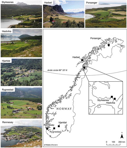
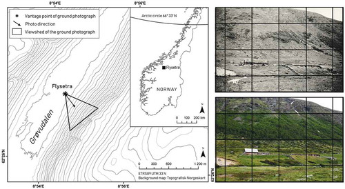
Seven landscape photographs from different locations in Norway were selected to evaluate the accuracy of spatial data obtained from georeferenced photographs (Figure 1). All photographs were taken by the Norwegian Institute of Bioeconomy Research (NIBIO) between 2004 and 2018 as part of the repeat photography project ‘Norwegian Landscapes in Retrospect’ (Tilbakeblikk) (Puschmann et al. 2006) and the 3Q-monitoring program (Dramstad et al. 2002). Photographs were captured with a Canon EOS 1DS (2004), EOS 5D (2009–2017) and EOS 6D (2018). Quantitative analysis of repeat photographs requires that the second photograph is taken from exactly the same position as the first photograph. In order to reconstruct the original vantage point with high precision, the original photograph is overlaid with a grid, which corresponds to the internal grid of the camera. The lines and crossing points of the grid allow to easily check the current view with the photograph and to adjust the position accordingly. To achieve a perfect alignment between both photographs, they are digitally aligned with each other through semi-transparent overlay in Adobe Photoshop. A more detailed description of the method is given in Bayr and Puschmann (2019). In addition to each terrestrial photograph, a corresponding vertical aerial photograph of the same area and from approximately the same year (± 1 year) was chosen. The 1937-photograph from Flysetra in Grøvudalen was provided by Sunndal municipality in digital form (jpeg, 400dpi). The repeat photograph in 2012 was taken by NIBIO using the same grid-method described above. The grid overlay is also illustrated in Figure 3. The ground photographs were supplemented by an aerial photograph from 1971, as the oldest available one, and a more recent aerial photograph from 2010.

Figure 1. Location of the seven landscape photographs which were used to evaluate the accuracy of geospatial data with the WSL Monoplotting Tool

2.2. Georeferencing of landscape photographs

The WSL Monoplotting Tool (WSL-MPT, version 2.0.0), developed by the Swiss Federal Research Institute WSL (Bozzini et al. 2012), was used to georectify the seven landscape photographs. The georectification process is based on three main components: 1) the oblique landscape photograph, 2) a digital terrain model (DTM) and 3) the ground control points (GCPs). Additionally, an aerial photograph of the same area is required to identify suitable objects or landmarks that can serve as reference points. The DTM with 1 m resolution is based on airborne laser scanning and has a vertical accuracy of ±10 cm. In this study, each landscape photograph was rectified based on 12 GCPs, which could be identified both in the landscape photograph and the corresponding aerial photograph. The software requires a minimum of five GCPs to perform the camera calibration. Former studies have performed the georectification based on six control points (e.g. Stockdale et al. 2015, McCaffrey and Hopkinson 2017). In the present study, 12 GCPs per image were chosen as this gave a more even distribution of points across the entire image. As emphasized by Hughes et al. (2006), Gindraux et al. (2017) and Oniga et al. (2018), it can be assumed that the accuracy increases with a higher number of GCPs, at least until a certain point before the effect flattens out. Typical reference points were solitary trees, stone blocks, road crossings, poles and building corners. In contrast to stereo-photogrammetry, monoplotting allows only to georeference points located directly on the earth’s surface, thus, GCPs where always digitized at the base of those objects. All 12 GCPs were then used to perform the camera calibration by calculating the intrinsic and extrinsic camera parameters. The monoplotting technique is based on the principle that the camera center and each pixel in the 2D photograph can be connected by a straight line. The continuation of this line intersects the DTM at the pixel’s corresponding 3D-position. The relationship between camera and the points can be described by a collinearity equation (Ghosh 2005, Bozzini et al. 2011):

$x_a-x_0=-c\frac{a_{11}\left(X-X0\right)+a_{21}\left(Y-Y0\right)+a_{31}\left(Z-Z0\right)}{a_{13}\left(X-X0\right)+a_{23}\left(Y-Y0\right)+a_{33}\left(Z-Z0\right)}$

$y_a-y_0=-c\frac{a_{12}\left(X-X0\right)+a_{22}\left(Y-Y0\right)+a_{32}\left(Z-Z0\right)}{a_{13}\left(X-X0\right)+a_{23}\left(Y-Y0\right)+a_{33}\left(Z-Z0\right)}$

where x0, y0 are the coordinates of the principal point (image center). X0, Y0, Z0 are the coordinates of the camera position. The values a₁₁ to a₃₃ are coefficients of a rotation matrix which define the camera orientation.

2.3. Accuracy test

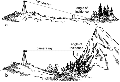
To test how the resolution of the chosen digital elevation model influences the quality of the georectification, the above-mentioned process was performed twice with the same GCPs but based on two different terrain models (DTM 1 m and DTM 10 m). Besides the 12 GCPs used for camera calibration and georectification, eight additional test points (total n = 56) and four polygons (total n = 28) were manually digitized on each photograph after successful georeferencing. The purpose of the test points was to test the accuracy of spatial data retrieved from the photographs on an independent set of vector data. For each of the digitized test points, the elevation difference between point and camera, distance to camera and angle of incidence was calculated. The angle of incidence (Figure 2) was calculated based on the average slope within a 10 m radius around each point as proposed by Stockdale et al. (2015). The accuracy of polygons was tested by comparing their mapped area on the georectified landscape photograph and the corresponding vertical aerial photograph. Accuracy was evaluated based on the following error measures:

• Theoretical 3D-error (in meters): describes the deviation between a point’s real-world coordinate and its projected coordinate as calculated during the camera calibration (Conedara et al. 2018). This error measure is automatically calculated by the WSL-MPT based on the GCPs and the collinearity equations.

• Point displacement (in meters): the Euclidean distance between the projected real-world position of a digitized point on the landscape photograph and its corresponding location on an aerial photograph. This measure is calculated from the manually digitized test points only and reflects the accuracy based on actual measurements (experimental error).

• Deviation in mapped area (in percent): difference between the projected area of polygons mapped on the georectified landscape photograph and the corresponding area mapped on an aerial photograph.

  Figure 2. The angle of incidence is defined as the angle between the ray from the camera and the earth’s surface at the point where the ray intersects the terrain. The angle of incidence depends on the local slope and the position of the camera. Terrestrial photographs taken in a flat landscape often show a low angle of incidence (a), while photographs in mountainous terrain can have large angles of incidence (b)

  

It should be noted that the theoretical 3D-error was only used for the GCPs, while the test points were evaluated based on an experimental error measure in order to gain a more realistic picture of the accuracies that can be expected from vector data.

Statistical analyses were performed in R version 3.6.1. Of particular interest for this study was to find out how the angle of incidence, distance to camera and the elevation difference affect accuracy. Linear regression was used to study the effects of these three parameters on the displacement of digitized points. Since the positive and continuous response variable showed a clear right-skewed distribution, a generalized linear model (GLM) with Gamma distribution and log-link function was chosen. The best model was determined using a stepwise forward-selection of explanatory variables.

2.4. Application example: Flysetra in Grøvudalen

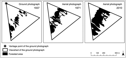
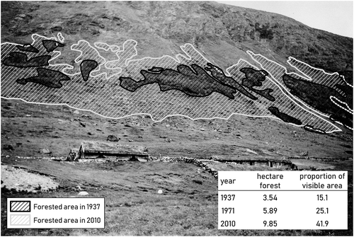
Grøvudalen is a small mountain valley in Sunndal municipality, Møre og Romsdal County in Mid-Norway and is part of the Dovrefjell–Sunndalsfjella National Park (Figure 3, left). Historically, Grøvudalen has been of major importance for summer pasturing and many of the traditional farm buildings are well preserved to this day thanks to conservation measures. One of those mountain farms is Flysetra (840 m.a.s.l.). The site was permanently inhabited until 1847. After that, the farm was still used for summer pasturing for a whole century (Mogstad 1964). The mountain farm was abandoned in the 1950s, but there is a limited amount of grazing activity in the valley until today. Probably due to the reduced agricultural activity in the area, the hillside has become gradually overgrown with mountain birch (Betula pubescens subsp. czerepanovii) and juniper (Juniperus communis) (Jordal and Bratli 2009). Repeat photography of the area close to the farm clearly illustrates the extent of forested area in the years 1937 and 2012 (Figure 3, right).

Figure 3. The abandoned mountain farm Flysetra in Grøvudalen. The black triangle in the map represents the viewshed of the visible area in the repeat photograph on the right. The photographs capturing Flysetra in a SE-direction were taken in 1937 by Halvor Vreim (with kind permission of Sunndal municipality) and in 2012 by Oskar Puschmann (NIBIO). The grid overlay demonstrates the technique that is used to identify the original vantage point of a photograph allowing to obtain perfectly aligned repeat photographs

In order to quantify the expansion of forest since 1937, the ground photographs were supplemented by an aerial photograph from 1971, as the oldest available one, and a second more recent aerial photograph from 2010. This allowed to go 73 years back in time and with that, to cover also the period when the farm still was actively used. By using the same procedure as for the accuracy test described above, the old photograph was processed with the WSL-MPT. Unfortunately, the scene from 1937 did not contain enough reference points that were still recognizable in the oldest available aerial photograph from 1971. Prominent stone blocks, for example, have disappeared due to the expanding woodland. To overcome this problem, the georectification was performed using the newer repeat photograph from 2012 together with the aerial photograph from 2010. Twelve GCPs were selected on the newer photograph and then transferred to the old photograph. The WSL-MPT does this automatically, if the newer photograph is replaced by the old one after successful camera calibration. This assumes that the repeat photographs were taken with high precision so that they overlay each other perfectly. After successful georeferencing, a viewshed of the visible section of the landscape in the photograph was created. Forest patches in the landscape photograph were digitized directly in the WSL-MPT and then exported to ArcGIS 10.7. Additionally, the forested areas in the two aerial photographs from 1971 and 2010 were manually digitized in ArcGIS. The analysis was limited to the viewshed-area of the ground photograph to allow a direct comparison of results from the different image sources.

3. Results

3.1. Accuracy of spatial data obtained from landscape photographs

The mean 3D-error over all seven images was 0.81 m if georectification was performed with a DTM of 1 m resolution (Table 1). Error values ranged from 0.03 m to a maximum of 2.33 m. If georectification was based on a 10 m DTM the mean 3D-error was 3.59 m, i.e. over four times higher. Still, even with the DTM 10 m, single points had very low errors, down to a minimum of 0.39 m. At the same time, the error values showed a large variation ranging up to a maximum error of 15.89 m.

Table 1. Difference in the theoretical 3D-error when georectification was based on a digital terrain model with 10 m or 1 m resolution, calculated for 12 ground control points per image

			DTM 10 m			DTM 1 m
Image	Terrestrial photo year	Aerial photo year	Mean 3D-error (m)	Min	Max	Mean 3D-error (m)	Min	Max
Rygnestad	2009	2010	3.07	0.43	12.01	0.81	0.04	1.79
Hadsel	2009	2008	3.73	0.39	12.63	1.17	0.28	2.33
Hestvika	2004	2004	3.09	0.74	6.87	0.74	0.03	1.86
Styrkesnes	2015	2015	4.05	1.61	11.23	0.66	0.08	1.57
Hjartdal	2018	2017	5.16	0.47	15.89	0.55	0.06	1.50
Porsanger	2016	2018	3.84	0.46	9.02	0.75	0.21	1.56
Rennesøy	2014	2013	2.20	0.46	5.39	0.97	0.32	1.79
average			3.59			0.81

The comparison of digitized points (n = 56) on both image sources resulted in a mean point displacement of 1.52 m (SD = 1.08) (Table 2). The lowest mean point displacement was 0.99 m (SD = 0.94) on the photograph from Porsanger, while the highest mean displacement with 2.89 m (SD = 1.43) appeared in the photograph from Hadsel (Figure 4). Effects on the accuracy of angle of incidence, distance to camera and elevation difference were tested. While distance to camera and elevation difference did not have significant effects, the angle of incidence showed a clearly significant effect (p < .001). The best model fit for the GLM was reached by including incidence angle as the only covariate (Figure 5).

Figure 4. Mean displacement of digitized points on a georectified landscape photograph compared to their corresponding position on an aerial photograph

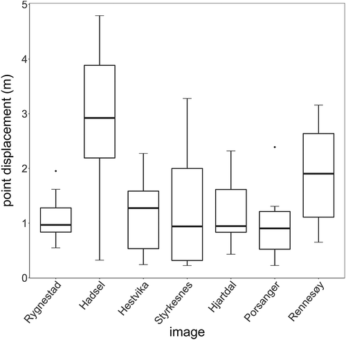
Figure 5. Relationship between the angle of incidence and point displacement as measured for 56 test points in seven landscape photographs

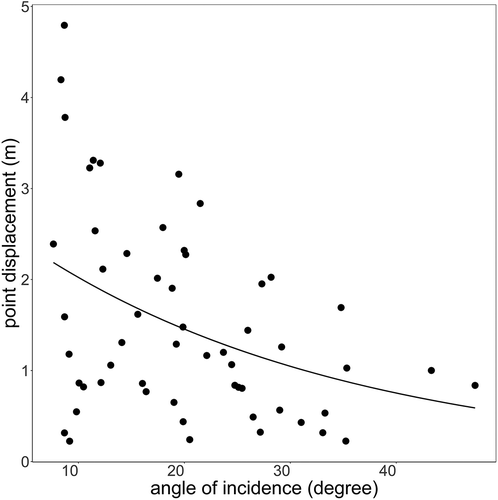
Table 2. Accuracy of points (8 per image, n = 56) and polygons (4 per image, n = 28) digitized on landscape photograph compared to their corresponding mapping on an aerial photograph

Image	Mean angle of incidence	Mean point displacement (m) (±SD)	Mean deviation in mapped area (%) (±SD)
Rygnestad	18.0°	1.11 (± 0.47)	6.21 (± 8.05)
Hadsel	13.7°	2.89 (± 1.43)	1.12 (± 0.95)
Hestvika	22.7°	1.19 (± 0.74)	3.78 (± 2.08)
Styrkesnes	13.3°	1.35 (± 1.26)	7.86 (± 4.88)
Hjartdal	24.3°	1.22 (± 0.66)	9.54 (± 4.75)
Porsanger	24.3°	0.99 (± 0.67)	5.58 (± 4.16)
Rennesøy	24.5°	1.88 (± 0.94)	4.90 (± 3.40)
All	20.1°	1.52 (± 1.08)	5.57 (± 4.77)

When areas were mapped, the size of polygons deviated on average with 5.57% (SD = 4.77) between the landscape photograph and the matching aerial photograph (Figure 6). With respect to area measurement, none of the explanatory variables showed a significant effect on accuracy. Nevertheless, many of the polygons digitized on terrestrial photographs showed a slight offset away from the camera. Figure 7 illustrates an example where polygon size is nearly the same, despite the clear horizontal displacement. Results for single points and polygons as well as the mapping results are provided as supplementary material to this article.

Figure 6. Mean deviation in size between polygons mapped on a georectified landscape photograph and the corresponding polygon on an aerial photograph

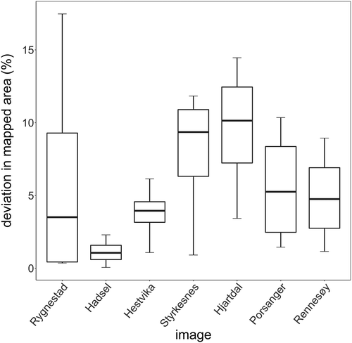
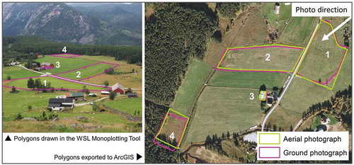
Figure 7. Comparison of mapped polygons on the photograph taken in Rygnestad. Polygon 1–3 show high correspondence between aerial photograph and georectified ground photograph. Polygon 4 shows a clear horizontal offset away from the camera. The vantage point is located outside of the visible section of the aerial photograph

3.2. Forest expansion at Flysetra in Grøvudalen

By combining the available ground photograph from 1937 with the aerial photographs from 1971 and 2010, it was possible to study forest expansion at Flysetra over a period of 73 years. As mentioned in the methods section, the old photograph offered some challenges for the georeferencing since the landscape scene did not contain enough reliable landmarks that could be identified in the oldest available aerial photograph from 1971. Instead, the georeferencing was successfully performed using the newer repeat photograph from 2012 and an aerial photograph from 2010. The total 3D-error of the 12 GCPs used for the georeferencing resulted in a mean 3D-error of 1.21 m (SD = 0.75).

Results show a pronounced spreading of mountain birch and juniper shrubs across the mountainside close to Flysetra during the study period (Figure 8). In 1937, based on the mapping performed on the georeferenced oblique photograph trees covered 3.5 ha, which represent 15.1% of the landscape section that is visible on the landscape photograph. According to Mogstad (1964), the farm was still used for summer grazing at this time, which explains the much more open character of the landscape in 1937 compared to later points in time. Since there exist no other image sources from 1937 that allows to verify the area estimates, we can instead make use of the experiences from the accuracy test. Based on the results for polygon features, we can expect a deviation of ±0.20 ha (corresponding to ±5.57%) in the mapped forest area. In 1971, the farm had already been abandoned for over a decade. At this stage, forest covered 25.1% (5.9 ha) of the area. In 2010, the farm had been abandoned for nearly 60 years and forest occupied 41.9% (9.9 ha) of the area. Summarized over the whole period from 1937 to 2010, the forested area in this case study landscape increased by 183.9%.

Figure 8. Forest expansion at Flysetra in Grøvudalen. The original situation in 1937 was digitized on the georectified ground photograph and then re-projected to the orthogonal perspective in order to compare it with aerial photographs

Finally, the results were visualized using the ‘world-to-pixel’ function in the WSL-MPT (Figure 9). This allowed the digitized areas from both the ground photograph and the aerial photographs to be combined into the ground view perspective and superimposed on the historical photograph from 1937. For the sake of clarity, the state in 1971 was not included. The result is an easily comprehensible illustration of landscape changes supplemented by quantitative measurements of real area cover changes.

Figure 9. The extent of forest in 1937 and 2010 visualized on the historical photograph from 1937 using the integrated world-to-pixel function of the WSL-MPT

4. Discussion

4.1. Landscape photographs as geospatial data source

Results of this study show that geospatial data extracted from georeferenced landscape photographs can be obtained with high accuracies. The measured theoretical 3D-errors for points lie in a range similar to the accuracy values reported by Conedara et al. (2018) who used the WSL-MPT to analyze natural hazard events in Switzerland. At the same time, the error values are considerably lower than the results gained by Stockdale et al. (2015) and McCaffrey and Hopkinson (2017). This difference might be explained by the characteristics of the photographic material. Both these studies used images from the Canadian Mountain Legacy Project which are primarily taken from highly elevated locations (e.g. mountain tops) and cover large parts of the surrounding landscape. In contrast, images in the Norwegian repeat photography collection are taken from less elevated spots capturing smaller and more detailed sections of the landscape. One can imagine that inaccurately placed points may result in larger errors if the photograph (and each pixel) covers a larger part of the landscape compared to a photograph that covers only a small area. Hence, we can assume that the general characteristics and scale of the photographic collection affects the magnitude of error values.

To achieve a high level of accuracy, some general key aspects need to be considered. An important factor is the quality of the DTM. The comparison of two different DTM resolutions (1 m versus 10 m) demonstrated the importance of a high-resolution terrain model for the accuracy of the georectification. In this regard, also the vertical accuracy of the DTM needs to be considered, which is closely related to its horizontal resolution. The DTM 1 m based on laser scanning is with ±10 cm relatively accurate and hence, is expected to have little influence on the accuracy of extracted geospatial data. In contrast, a DTM with 10 m resolution generalizes the earth’s surface much stronger and thus, can deviate up to several meters from the real surface. A visual comparison of the two DTM resolutions and the resulting elevation differences for the example at Flysetra is included in the supplementary material (Supplement 4). However, it is important to remember that the given vertical accuracy for a dataset is only an average that can show large site-specific variations. Nevertheless, even if no 1 m DTM is available for the region of interest, the WSL-MPT can still be used with a coarser terrain model (e.g. 10 m), but larger uncertainties related to the extracted information should be expected.

Another problem related to terrain data is that these data sets are rarely updated. With increasing time difference between the generation of the terrain model and the landscape photograph, it becomes more likely that geomorphological processes may have altered the surface (James et al. 2012). Although the shape of the terrain seems to be stable over long time, the earth’s surface changes either gradually due to erosion or ground subsidence, or more sudden due to landslides and human activities. However, this limitation applies in the same way to geospatial analyses based on aerial photographs and is therefore not a specific problem of terrestrial photographs.

The second critical aspect is the placement and distribution of GCPs. The precise linkage between a reference point in the landscape photograph and its corresponding real-world location is a crucial precondition for acquiring accurate geospatial data. Due to the oblique perspective, even small inaccuracies in placing a point can lead to a large horizontal displacement. Objects with sharp edges such as buildings or street corners as well as small and well-defined objects such as energy poles make it easier to place GCPs precisely. Hughes et al. (2006) emphasize that a higher density of GCPs in the area of interest can increase the accuracy of spatial measurements. However, even if the calibration process results in a low theoretical 3D-error, this does not necessarily mean that spatial data extracted from the photographs reach the same accuracy. This is proven by the fact that the actually measured errors of the additionally digitized points were larger than the theoretical error. During the camera calibration, the algorithm tries to find the optimal parameters for the collinearity equations so that the mean error of all GCPs is minimized. The final transformation does rarely represent a perfect fit for the entire photograph, particularly in areas with a strong topography. This explains why points digitized after finished georeferencing can have larger errors compared to the points used as GCPs for the calibration procedure (Hughes et al. 2006).

The results of this study indicate that a low angle of incidence can entail a larger spatial error, which is supported by the findings of Stockdale et al. (2015). This effect is the reason why data retrieved from orthogonal aerial photographs are generally more accurate than data from oblique photographs. However, mountainous regions constitute an exception. Very steep areas are usually underestimated in orthogonal aerial photographs since the angle of incidence between sensor and the earth’s surface can become very low. In contrast, an oblique photograph capturing a steep mountain side can reach a very large angle of incidence and thus obtain more accurate results than the corresponding image taken from above (Sanseverino et al. 2016, Fortin et al. 2018). The relation between angle of incidence and topography is apparent also in Figure 2.

Unlike Stockdale et al. (2015), but equal to the findings of McCaffrey and Hopkinson (2017), the present study did not reveal a significant effect of distance to camera. Nevertheless, it is likely that it has an influence on accuracy as well. Stockdale et al. (2015) points out that more distant objects appear very small and often suffer from pixelation, which makes it difficult to place the cursor precisely. It also turned out to be unfavorable to place points close to ridges, where the risk is high that small inaccuracies in the DTM lead to large horizontal displacement. The same effect appeared in the mapping of areas on oblique photographs, where results showed that polygons were prone to a slight horizontal offset away from the camera. This effect appeared not to be systematic and rather marginal, but it seemed to mainly affect polygons further away from the camera. This suggests that the offset might be caused by inaccuracies in the digitalization. Nevertheless, with respect to area measurements, the percent difference between areas mapped on aerial and landscape photographs were within a reasonable margin of around ±5%.

At this point, it must be emphasized that the given accuracy measures in this study do not relate to the deviation of digitized features from their real-world position, but instead the deviation from their corresponding location and measurement on the aerial photograph. This distinction is important because the aerial photograph itself holds some degree of spatial error, inherited from the orthorectification process. To evaluate the deviation from real-world coordinates would require measuring the precise location of each point and polygon in the field.

4.2. Limitations and opportunities of using georectified landscape photographs

One of the main challenges of using oblique ground-level photographs is that parts of the landscape can be hidden behind buildings, trees or ridges. If obstacles are very close to the camera and thus, take up a large part of the view, the photograph is rarely suited for monoplotting. Particularly in repeat photographs, it is a frequent phenomenon that vegetation has grown much higher and denser since the first photograph making it inappropriate for monoplotting. In this case, only the historical photograph might be georectified using the WSL-MPT and then combined with more recent aerial photographs to assess changes. Another issue is that areas on back-facing slopes are not captured from the photographer’s viewpoint. Hence, the mapping based on oblique photographs should be restricted to the visible area using viewshed analysis. However, even within the visible part of the landscape high vegetation and other objects can lead to over- or underestimation of certain land cover types. For example, a wooded patch in the oblique perspective might appear as a dense forest, while it actually could be permeated with open spaces like meadows or water bodies.

A high angle of incidence, for example if the photograph is taken from the top of a hill, can to a certain degree mitigate the effect of blocking. Still, in photographs with high vegetation the possibilities to map larger continuous areas will be limited. Thus, monoplotting seems to be most suitable for open landscapes, for example those, which are dominated by agriculture. In this regard, historical photographs have the advantage that the agricultural landscape, in general, was much more open. This was due to wood being an intensively used raw material and because grazing in the outfields was much more common. For more recent times and as far as available, aerial photographs are a better choice for quantifying landscape change as they are easier to analyze, cover a much larger area and show the landscape in an orthogonal and unobstructed view (Frankl et al. 2011). However, with their high level of detail, ground photographs can supplement aerial photographs with additional information about the quality of land cover. For example, Ode et al. (2010) point out, that early stages of succession after abandonment may not be visible from aerial photographs but can be clearly identified in ground photographs. Terrestrial photographs may also serve as a cheap and flexible alternative if aerial images do not exist for a certain area (Kull 2005).

Unquestionably, the greatest benefit of landscape photographs is their temporal range. Historical photographs from the time before aerial photography can add valuable information which would otherwise not exist (Gimmi et al. 2016). The example from Flysetra demonstrated well how the research period could be extended by combining multiple data sources, in this case aerial and terrestrial photographs. Thanks to the historical photograph, it was possible to cover a period of more than 70 years and through that also the state when the mountain farm was still actively used for summer grazing. When the first aerial photograph was taken in 1971, the farm had already been abandoned for more than a decade. The reduced agricultural activity in the area has presumably allowed woody vegetation to spread across the mountainside. The spreading of forest into former pastures is characteristic for many other landscapes of Norway, a trend which is well documented in thousands of photographs reaching back until the late nineteenth century. Within the Tilbakeblikk-project (Puschmann et al. 2006), many of those old photographs have been retaken from exactly the same position.

In this regard, the example made clear how repeat photography can contribute to the selection of appropriate GCPs. The time difference between modern aerial photographs and many historical photographs can make it difficult to find enough reliable reference points. To solve this problem, the georectification can be performed based on a repeat photograph and then transferred to the historical photograph. Of course, this assumes that repeat photographs are taken with high precision to enable their exact overlay.

Another significant advantage of monoplotting is that it offers alternative ways to visualize geospatial data. For example, areas and objects originally mapped on vertical remote sensing imagery can be projected into the ground-level perspective and then be visualized on top of a landscape photograph. In Norway, experiences show that the use of repeat photographs represents an effective way to communicate landscape change to a broad audience (Bayr and Puschmann 2019). This is because the oblique perspective of landscape photographs has the advantage of being much closer to how people naturally perceive landscapes. This allows the understanding of landscape dynamics even without the need of having experience in interpreting maps and aerial photographs. Through this, repeat photography can considerably contribute to an increased public and political awareness of how the cultural landscape has changed as a result of changes in land management practices over time.

4.3. Future possibilities

The number of historical landscape photographs stored in public and private archives is immense. By using the monoplotting method to georectify this unique material, we can achieve quantitative information on landscape change which have not been available before. This example also shows that new methods and technologies does not only provide constantly new and better imagery, but that we also can turn back and apply these new methods to exploit the unused potential of more traditional image sources, that may nowadays appear somewhat obsolete. The focus of this study was on using the WSL-MPT on oblique photographs taken at the ground-level. Nevertheless, the monoplotting method could also be useful for the analysis of historical oblique aerial photographs. For example, the Norwegian private airline company ‘Widerøe’ captured between the late 1930s and 70s oblique aerial photographs at very low altitudes. These photographs focused on individual houses and properties, mainly farms and the surrounding landscape. In contrast to vertical photographs, which are commonly used for land surveying and mapping, the purpose of such oblique aerial photographs was first and foremost to sell them on the doorstep to the owners (Hansen 2012). This kind of commercial use of aerial photographs was very common in many developed countries at this time (Svenningsen et al. 2015). Today, many of those oblique photographs are scanned and publicly available in digital archives. Since they lack georectification and are taken at an oblique angle, they are very similar to non-rectified landscape photographs. Therefore, monoplotting might be a suitable method also for the quantitative study of oblique aerial photographs.

5. Conclusion

Landscape photographs represent a valuable source of information on historical landscape change. Still, there exist only limited experience on how confident mappings based on oblique photographs really are. The primary aim of this study was to test the potential of landscape photographs to provide accurate geospatial data using the WSL Monoplotting Tool. The results showed that it is possible to obtain geographical data of high spatial accuracy. An important precondition however was the use of a DTM with high resolution and a careful placement and distribution of GCPs. A high angle of incidence between the camera ray and the earth’s surface had a significant positive effect on accuracy. Besides this, it became obvious that also the characteristics and scale of the used photographic material itself influences the magnitude of the error values. Repeat photography proved to be particularly advantageous for the georectification process when the landscape had changed so much that it was difficult to select reliable reference points. Due to the absence of any other image source before the invention of aerial photography, it seems to be acceptable that oblique photographs provide slightly less accurate data than vertical aerial photographs. Although oblique photographs cannot compete with the spatial accuracy of undistorted top-view imagery, they can contribute with other benefits such as a high spatial and temporal resolution as well as their ability to communicate landscape change in a clear and comprehensible manner. Through this, landscape photographs contribute substantially to make research on landscape dynamics and land use change more accessible to the general public.

Acknowledgments

This work was supported by the Norwegian Ministry of Agriculture and Food through the Research Council of Norway [nr. 194051]. Many thanks to Oskar Puschmann (NIBIO) for providing the repeat photographs used in this study and to Sunndal Municipality for the 1937-photograph. I also thank Geir Harald Strand and Wenche Dramstad (both NIBIO), as well as Bernd Etzelmüller (University of Oslo) for their valuable support during the project. I am also grateful to the editor and the anonymous reviewers for their helpful suggestions.

Disclosure statement

No potential conflict of interest was reported by the author

Data and codes availability statement

The data and codes that support the findings of this study are available in figshare.com with the identifier https://doi.org/10.6084/m9.figshare.c.4973372

Supplementary material

Supplemental data for this article can be accessed here.

Additional information

Funding

This work was supported by the Research Council of Norway [194051].

Notes on contributors

Ulrike Bayr

Ulrike Bayr is a PhD student in the Landscape Monitoring section at Norwegian Institute of Bioeconomy Research (NIBIO) in Ås. She has an MSc in physical geography with a specialization in GIS and remote sensing from the University of Tübingen, Germany. Her research interests focus on topics related to landscape change, vegetation dynamics and landscape ecology.

References

- Almås, R. and Campbell, H., eds., 2012. Rethinking agricultural policy regimes: food security, climate change and the future resilience of global agriculture. Bingley, UK: Emerald Publishing.
- Bayr, U. and Puschmann, O., 2019. Automatic detection of woody vegetation in repeat landscape photographs using a convolutional neural network. Ecological Informatics, 50, 220–233. doi:https://doi.org/10.1016/j.ecoinf.2019.01.012
- Bozzini, C., Conedera, M., and Krebs, P., 2011. A new tool for obtaining cartographic georeferenced data from single oblique photos. In: K. Pavelka, ed. Proceedings of CIPA Symposium 23, 12–16 September 2011. Prague.
- Bozzini, C., Conedera, M., and Krebs, P., 2012. A new monoplotting tool to extract georeferenced vector data and orthorectified raster data from oblique non-metric photographs. International Journal of Heritage in the Digital Era, 1 (3), 499–518. doi:https://doi.org/10.1260/2047-4970.1.3.499
- Bühler, Y., et al., 2019. Where are the avalanches? Rapid SPOT6 satellite data acquisition to map an extreme avalanche period over the Swiss Alps. The Cryosphere, 13 (12), 3225–3238. doi:https://doi.org/10.5194/tc-13-3225-2019
- Clark, P.E. and Hardegree, S.P., 2005. Quantifying vegetation change by point sampling landscape photography time series. Rangeland Ecology and Management, 58 (6), 588–597. doi:https://doi.org/10.2458/azu_rangelands_v58i6_hardegree
- Conedara, M., et al., 2018. Using the Monoplotting Technique for Documenting and Analyzing Natural Hazard Events. Natural Hazards, 64 (3), 1969–1975. doi:https://doi.org/10.5772/intechopen.77321
- Dramstad, W.E., et al., 2002. Development and implementation of the Norwegian monitoring programme for agricultural landscapes. Journal of Environmental Management, 64 (1), 49–63. doi:https://doi.org/10.1006/jema.2001.0503
- Fortin, J.A., et al., 2018. Estimates of landscape composition from terrestrial oblique photographs suggest homogenization of Rocky Mountain landscapes over the last century. Remote Sensing in Ecology and Conservation, 5 (3), 224–236. doi:https://doi.org/10.1002/rse2.100
- Frankl, A., et al., 2011. Linking long-term gully and river channel dynamics to environmental change using repeat photography (Northern Ethiopia). Geomorphology, 129 (3–4), 238–251. doi:https://doi.org/10.1016/j.geomorph.2011.02.018
- Gabellieri, N. and Watkins, C., 2019. Measuring long-term landscape change using historical photographs and the WSL Monoplotting Tool. Landscape History, 40 (1), 93–109. doi:https://doi.org/10.1080/01433768.2019.1600946
- Ghosh, S.K., 2005. Fundamentals of computational photogrammetry. New Delhi: Concept Publishing Company.
- Gimmi, U., et al., 2016. Assessing accuracy of forest cover information on historical maps. Prace Geograficzne, 146, 7–18. doi:https://doi.org/10.4467/20833113PG.16.014.5544
- Gindraux, S., Boesch, R., and Farinotti, D., 2017. Accuracy assessment of digital surface models from unmanned aerial vehicles’ imagery on glaciers. Remote Sensing, 9 (2), 186. doi:https://doi.org/10.3390/rs9020186
- Hall, F.C. 2001. Ground-based photographic monitoring. General Technical Report. PNW-GTR-503. Portland: U.S. Department of Agriculture, Forest Service, Pacific Northwest Research Station. doi:https://doi.org/10.2737/PNW-GTR-503
- Hansen, M.D., 2012. Luftfotografiets vej til succes [The success of aerial photography]. Magasin fra Det Kongelige Bibliotek, 25 (4), 32–38. Available from: https://tidsskrift.dk/magasin/article/view/66747.
- Hastings, J.R. and Turner, R.M., 1965. The changing mile. Tucson: University of Arizona Press.
- Hendrick, L.E. and Copenheaver, C.A., 2009. Using repeat landscape photography to assess vegetation changes in rural communities of the Southern Appalachian Mountains in Virginia, USA. Mountain Research and Development, 29 (1), 21–29. doi:https://doi.org/10.1659/mrd.1028
- Herrero, H.V., et al., 2017. Using repeat photography to observe vegetation change over time in Gorongosa national park. African Studies Quarterly, 17 (2), 65–82. Available from: http://www.africa.ufl.edu/asq/v17/v17i2a4.pdf
- Hughes, M.L., McDowell, P.F., and Marcus, A., 2006. Accuracy assessment of georectified aerial photographs: implications for measuring lateral channel movement in a GIS. Geomorphology, 74 (1–4), 1–16. doi:https://doi.org/10.1016/j.geomorph.2005.07.001
- James, L.A., et al., 2012. Geomorphic change detection using historic maps and DEM differencing: the temporal dimension of geospatial analysis. Geomorphology, 137 (1), 181–198. doi:https://doi.org/10.1016/j.geomorph.2010.10.039
- Jordal, J.B. and Bratli, H. 2009. Skjøtsel og overvåking av biologisk verdifullt kulturlandskap i Grøvudalen, Sunndal [Management and monitoring of biologically valuable cultural landscapes in Grøvudalen, Sunndal]. Sunndal kommune og Sunndal beitelag, Report no. 1. Available from: http://www.jbjordal.no/publikasjoner/Grovudalen_Skjotsel_2009.pdf
- Kaim, D., 2017. Land cover changes in the polish Carpathians repeat photography. Carpathian Journal of Earth and Environmental Sciences, 12, 485–498.
- Klett, M., Manchester, E., and Verburg, J., 1984. Second view: the rephotographic survey project. Albuquerque: University of New Mexico Press.
- Kolecka, N., et al., 2015. Mapping secondary forest succession on abandoned agricultural land with LiDAR point clouds and terrestrial photography. Remote Sensing, 7 (7), 8300–8322. doi:https://doi.org/10.3390/rs70708300
- Kull, C.A., 2005. Historical landscape repeat photography as a tool for land use change research. Norsk Geografisk Tidsskrift - Norwegian Journal of Geography, 59 (4), 253–268. doi:https://doi.org/10.1080/00291950500375443
- Manier, D.J. and Laven, R.D., 2002. Changes in landscape patterns associated with the persistence of aspen (Populus tremuloides Michx.) on the western slope of the Rocky Mountains, Colorado. Forest Ecology and Management, 167 (1–3), 263–284. doi:https://doi.org/10.1016/S0378-1127(01)00702-2
- Masubelele, M.L., Hoffman, M.T., and Bond, W.J., 2015. A repeat photography analysis of long‐term vegetation change in semi‐arid South Africa in response to land use and climate. Vegetation Science, 26 (5), 1013–1023. doi:https://doi.org/10.1111/jvs.12303
- McCaffrey, D.R. and Hopkinson, C., 2017. Assessing fractional cover in the Alpine treeline ecotone using the WSL monoplotting tool and airborne lidar. Canadian Journal of Remote Sensing, 43 (5), 504–512. doi:https://doi.org/10.1080/07038992.2017.1384309
- McCaffrey, D.R. and Hopkinson, C., 2020. Repeat oblique photography shows terrain and fire-exposure controls on century-scale canopy cover change in the Alpine treeline ecotone. Remote Sensing, 12. doi:https://doi.org/10.3390/rs12101569
- Michel, P., Mathieu, R., and Mark, A.F., 2010. Spatial analysis of oblique photo-point images for quantifying spatio-temporal changes in plant communities. Applied Vegetation Science, 13 (2), 173–182. doi:https://doi.org/10.1111/j.1654-109X.2009.01059.x
- Mogstad, L., 1964. Oversyn over fjellbeite i Møre og Romsdal [Overview of mountain pastures in Møre og Romsdal county]. Norske fjellbeite Vol. 10. Oslo: Det kgl. selskap for Norges vel.
- Ode, Å., Tveit, M.S., and Fry, G., 2010. Advantages of using different data sources in assessment of landscape change and its effect on visual scale. Ecological Indicators, 10 (1), 24–31. doi:https://doi.org/10.1016/j.ecolind.2009.02.013
- Oniga, V.E., Breaban, A.I., and Statescu, F., 2018. Determining the optimum number of ground control points for obtaining high precision results based on UAS images. Proceedings, 2 (7), 352. doi:https://doi.org/10.3390/ecrs-2-05165
- Pickard, J., 2002. Assessing vegetation change over a century using repeat photography. Australian Journal of Botany, 50 (4), 409–414. doi:https://doi.org/10.1071/BT01053
- Puschmann, O., Dramstad, W.E., and Hoel, R., 2006. Tilbakeblikk: norske landskap i endring. [Flashback: Norwegian landscapes in retrospect]. Oslo: Tun Forlag.
- Roush, W., Munroe, J.S., and Fagre, D.B., 2007. Development of a spatial analysis method using ground-based repeat photography to detect changes in the alpine treeline ecotone, Glacier National Park, Montana, USA. Arctic, Antarctic, and Alpine Research, 39 (2), 297–308. doi:https://doi.org/10.1657/1523-0430(2007)39[297:DOASAM]2.0.CO;2
- Sanseverino, M.E., Whitney, M.J., and Higgs, E.S., 2016. Exploring landscape change in mountain environments with the mountain legacy online image analysis toolkit. Mountain Research and Development, 36 (4), 407–416. doi:https://doi.org/10.1659/mrd-journal-d-16-00038.1
- Scapozza, C., et al., 2014. Assessing the rock glacier kinematics on three different timescales: a case study from the southern Swiss Alps. Earth Surface Processes and Landforms, 39 (15), 2056–2069. doi:https://doi.org/10.1002/esp.3599
- Stoate, C., et al., 2009. Ecological impacts of early 21st century agricultural change in Europe – A review. Journal of Environmental Management, 91 (1), 22–46. doi:https://doi.org/10.1016/j.jenvman.2009.07.005
- Stockdale, C.A., et al., 2015. Extracting ecological information from oblique angle terrestrial landscape photographs: performance evaluation of the WSL Monoplotting Tool. Applied Geography, 63, 315–325. doi:https://doi.org/10.1016/j.apgeog.2015.07.012
- Stockdale, C.A., Macdonald, S.E., and Higgs, E., 2019. Forest closure and encroachment at the grassland interface: a century-scale analysis using oblique repeat photography. Ecosphere, 10 (6). doi:https://doi.org/10.1002/ecs2.2774
- Svenningsen, S.R., et al., 2015. Historical oblique aerial photographs as a powerful tool for communicating landscape changes. Land Use Policy, 43, 82–95. doi:https://doi.org/10.1016/j.landusepol.2014.10.021
- Webb, R.H., Boyer, D.E., and Turner, R.M., eds., 2010. Repeat photography: methods and applications in the natural sciences. Washington: Island Press.
- Westoby, M.J., et al., 2012. Structure-from-Motion photogrammetry: A low-cost, effective tool for geoscience applications. Geomorphology, 179, 300–314. doi:https://doi.org/10.1016/j.geomorph.2012.08.021
- Wiesmann, S., et al. 2012. Reconstructing historic glacier states based on terrestrial oblique photographs. Proceedings of the AutoCarto International Symposium on Automated Cartography, Columbus, OH, USA.