Mapping research networks supported by the National Geographic Society through spatial social networks

ABSTRACT

Research is an interconnected global endeavor. Networks of research collaborations are often using Social Networks Analysis. Its variant Spatial Social Networks allowing explicit embedding of spatial information in the network. Variations in incorporating spatial information results in multiple conceptualizations of networks, enabling exploration of a variety of questions regarding collaborations. To elucidate this approach the National Geographic Society grants database (1890–2016) is utilized to create three different networks that embed spatial information in distinct ways. Each network highlights a different aspect of connectivity latent in the dataset and along with the spatial information, emphasizes international and regional trends of collaborations. The networks explicate the international nature of collaborative research by virtue of people collaborating explicitly, or by working in the same places. It also highlights the multidisciplinary nature of research in various countries, and how it can be useful to ideate about new projects. Additionally, the network approach highlights the dominance of global north in conducting fieldwork-based research across the world, mostly through collaborations. The abstraction afforded by social network models requires further deliberation on the way spatial relationships can be captured differently using the node-edge structure and how these alternate networks compare to traditional networks in GIScience.

KEYWORDS:

• Spatial Social Networks
• giscience
• international collaboration

1. Introduction

Research is increasingly seen as an interconnected enterprise between scholars via collaborations in publications, grants, and presentations at conferences, often transcending regional and national boundaries. This increasingly international and interdisciplinary nature of research frequently dominates discussions around academic endeavors in the age of globalization (Batty 2003). The discussions are further bolstered by statements such as ‘the best science comes from international collaborations’, backed by a scrutiny of three decades of journal articles (Adams 2013, p. 557). The preferred method of analyzing the nature of collaborations is through modeling co-authorship or citations as a ‘social network’ (Kretschmer 1997, Otte and Rousseau 2002, Wagner and Leydesdorff 2005, Hou et al. 2008, Wagner et al. 2015, Leydesdorff et al. 2018). Here this avenue of research is expanded by studying various forms of collaborations that can only be understood through the incorporation of spatial information as a key determinant of interactions and consequently, collaborations.

A social network describes collaborations using nodes (representing scholars) connected via edges representing the conceptual relationships (e.g., co-authorship, citation). Within Geography, social network analysis (SNA) methods have been utilized to analyze the within and between country interactions at the Annual Meeting of the American Association of Geographers (Derudder and Liu 2016), as well as to understand the growth of the field of GIScience (Sun and Manson 2011). The former showed that while international participation has increased at the meeting between 2005 and 2013, the nature of the papers and sessions have in fact become more inward looking, with more intra-national interactions as opposed to international ones. The latter examined authorship-based collaborations and identified three trends in GIScience research: increased co-authorships, adoption of GIScience software in other fields, and increased internal cohesion and maturity of the field. To further understand the concept of ‘community’ of GIScience scholarship, Mao (2014) highlights the ‘scale-free’ nature of collaborations and citations in the field, which implies an uneven geographic distribution of GIScience and System research organizations across the United States of America (US) with a predominance of clustered spatial interactions between them.

SNA focuses primarily on the node-and-edge topological structure to model the relationships in systems or societies with little regard to the spatial location of the node, edges, and the network (Andris 2016, Sarkar et al. 2016). However, recently the spatial aspects of social networks have garnered a great deal of interest (Barthélemy 2011, Andris et al. 2018, Sarkar et al. 2019). Various studies have re-iterated the probability of social ties decreasing exponentially with increase of distance (Liben-Nowell et al. 2005, Wong et al. 2006, Preciado et al. 2011, Scellato et al. 2011). Geographic applications of SNA include epidemiology (Keeling et al. 2011, Giebultowicz et al. 2011a, 2011b, Emch et al. 2012), criminology (Radil et al. 2010), trade networks (Castells 1996, Fleming and Sorenson 2001, Owen-Smith and Powell 2004), as well as co-operative agriculture practices (Faust et al. 2000, Entwisle et al. 2007, Abizaid et al. 2015, 2016), and the position of cities in a global network (Liu and Derudder 2012, Derudder et al. 2013), to highlight a few. This view disregards the multiplicity of interactions that can be represented using the edges leading to modeling diverse relationships within the same dataset (Liu and Derudder 2013, Ye and Liu 2018) and the opportunity to incorporate spatial information as part of the edges or the network a whole.

This article demonstrates how different spatial social networks (SSNs) can be created from a single dataset that embeds spatial information in distinct forms to model various spatial relationships. A database of awarded research grants from National Geographic Society (NGS) is used to emphasize how embedding the spatial information differently results in varied network conceptualizations, which then allows the exploration of a variety of questions regarding research collaborations. The network approach allows exploration beyond the first-degree connections to understand where each entity fits into the larger fabric of a research network. Operationalizing different spatial relationships through the network structure goes beyond the commonly used but restrictive ‘location anchored node model’. This allows the use of networks as an epistemology capable of modeling, analyzing, and explaining both spatial and non-spatial relationships intrinsic to systems where interaction plays an important part (Buch-Hansen 2014, Alfano et al. 2018).

It is understood that the nature of the NGS database is biased toward grants obtained by North American scholars, the region where the majority of the applications come from; however, the focus of this paper is to explore new methods of developing networks. Thus, while the insights obtained are constrained by the specific nature of the dataset, the conceptualizations nonetheless present interesting insights regarding funding-driven international collaborations, primarily in disciplines where there tends to be fieldwork involved. These network models can be used to evaluate any system where spatial information is crucial for understanding relationships.

2. Social networks, relational multiplicity and incorporation of spatial information in social networks

Several linear and interconnected geographic entities (e.g., roads, rivers) are often conceptualized as a topological network. In addition to topology, real-world physical networks (e.g. roads, utility) studied by geographers have important topographical considerations as both the nodes and edges are embedded in geographic space. Exploiting both topological and topographical information has been shown to provide insights into the dynamics of urban structure (Mossa et al. 2005, Porta et al. 2006, Zhong et al. 2014), even though the topological signatures of road networks across the world show remarkable quantitative similarities (Jiang 2007).

The definition of the term ‘social network’ as a collection of discrete entities (depicted as nodes) that are strung together by edges (representing relationships) is intuitive and flexible. Given a set of distinguishable entities and some relationship between them, SNA can be used to model many real-world systems. However, in a given set of entities, there can be multiple relationships between them, and each relationship can be used to construct a different network (Zuckerman 2008, Liu and Derudder 2013). For example, given a set of people, the different relationships can be kinship or friendship and either can be modeled as a network. Therefore, it is important to precisely define what an edge (or connection) consists of, and what it represents.

Enriching the node-edge topological model with attribute data can aid in gaining further insight into social network processes, like attribute-based homophily (McPherson et al. 2001). In addition to attaching attributes like age and sex, spatial information has also been added to facilitate understanding spatial aspects of the network (Andris 2016, Sarkar et al. 2019). Adding spatial information to the network also facilitates operationalizing topological connections beyond spatial relationships in Euclidean space (Egenhofer and Franzosa 1991), a realization that remains difficult in GISystems. The dominant way of handling spatial information in SNAs (referred to as Spatial Social Networks, or SSNs) is to incorporate spatial information as an attribute of the nodes (Sarkar et al. 2016). If the relationship between the nodes is a spatial one, then it is possible to encode spatial information in the edges of the network too. Since multiple spatial relationships can be present in any given dataset, it is possible to create multiple network-based representations that capture spatial information as part of nodes, edges, or both. Hence, networks created from the same dataset can provide different views of the various latent spatial relationships. The conceptualization of these networks with spatial information embedded in various ways forms the focus of this article. The flexibility of social networks to model different relationships (spatial and non-spatial) between entities opens up possibilities for incorporating spatial information in varied ways as part of the network to explore the complementary insights provided by the different conceptualizations.

3. Methods

A database of more than 12,000 records representing grants given by NGS between 1890 and early 2016 is used to build the networks. The number of grants given out annually are few in the early years (three in the first decade) but increased significantly over the years (more than 400 in 2015). The records consist of multiple columns, and the columns of interest are listed in Table 1. For creating the networks of interest, the entries that are related to non-country entities, e.g., ‘Space’, ‘Laboratory’ and ‘Oceans’, are discarded. Also, the long-time frame of the dataset means there are entries that may relate to different countries over time, for example ‘Serbia’ and ‘Serbia and Montenegro’. These are left untouched from their original presentation in the database. Since NGS is a US-based organization, the US is overrepresented in the dataset. Hence, the results of the analysis presented here need to be understood with this bias in mind.

Table 1. Fields of interest in the National Geographic Society grants database

Field Name	Description
Contact Primary Address Country	The country of the researcher’s primary affiliation.
Grant Discipline(s)	The discipline(s) of research. For most grants (70.4%), multiple disciplines are listed.
Fieldwork Location – Country	The country(s) where field work was carried out. Several grants (22.3%) have multiple entries for fieldwork country, implying that there were multiple field sites involved.
Fieldwork Location – Continent	The continent(s) where the field work was carried out. When the fieldwork location was located in different countries, the countries in question may be in different continents. The continents listed in the database used for the analysis in this paper are Africa (2894 instances), Asia (3348 instances), Europe (1198 instances), Oceania (1140 instances), North America (3448 instances), South America (2464 instances), and Central America (2231 instances). Other listings include Oceans (138 instances), Ocean Islands (34 instances), Space (24 instances), Worldwide (33 instances), and Laboratory/Archival Research Only (31 instances).

This article uses multiple network conceptualizations by considering different attributes of the database as either nodes or edges to answer three questions highlighted in Table 2. Table 2 also provides an overview of the various networks developed from the NGS grants database, depending on how spatial information is incorporated and the question about research collaborations that it primarily addresses. The answers to the questions predicated on the NGS dataset highlight the value of operationalization of various forms of SSNs.

Table 2. Overviews of the three different spatial social networks created

Network	Node	Node spatial?	Edge	Edge Spatial?	Question
1	Fieldwork Location (Country/Continent)	Yes	Same Grant	No	What is the ‘research connectivity’ between countries?
2	Principal Investigator’s Location	Yes	Fieldwork Location	Yes	How ‘internationalized’ is the research of the various PIs?
3	Discipline	No	Fieldwork Location	Yes	What is the multi-disciplinary research potential of different countries?

3.1. Network 1

In the Field Location-Grant Network, the nodes represent field work locations. In some grants, more than 10 locations are listed as the fieldwork country, however, for each row a maximum of first 10 entries is considered. Two locations are connected if they are mentioned simultaneously as fieldwork locations in grants. Thus, the nodes in the network represent fieldwork countries connected by edges representing co-mentions. The edges have weights which denote the number of times the two countries are mentioned together in a grant. For example, in Table 3B, Canada and Uganda are connected with a weight of 2, as the countries are simultaneously mentioned in Grant 1 and 6 in Table 3. The resulting network was not fully connected as entries like ‘Cape Evans’ and ‘Estonia’ only appeared in single grants, and these isolated nodes are discarded. The connected part of the network consists of 193 nodes and 1763 edges without self-loops or parallel edges (multiple edges connecting two nodes).

Table 3. Example illustrating how the nodes, edges, and edge weights are created for the different networks. The entries are created for the example and do not represent entries in the database. Table A depicts organization of entries in the database (transposed to show the column names in the first row). Table B shows the weighted undirected edgelist for Type 1 network with the spatial information in the nodes. Table C shows the weighted edgelist for Type 2 network with the spatial information in the form of country names attached to both the nodes and edges. Table D shows the weighted edgelist created by only using Fieldwork Country 1 for brevity. Type 3 network has spatial information in the form of edge attributes

(A)
Grant ID		1	2	3	4	5	6
Principal Investigator Country		Canada	India	Sweden	Ireland	India	Netherlands
Co-Applicant Country		India	Bhutan		Sweden, Netherlands	Nepal	Nepal
1^st Discipline		A	C	C	B	A	A
2^nd Discipline		E	B				C
3^rd Discipline		B					F
Fieldwork Country 1		Canada	India	Canada	Ireland	India	Canada
Fieldwork Country 2		Uganda	Bhutan	Sweden	Nepal	Brazil	Sweden
Fieldwork Country 3		Brazil	Nepal				Uganda
(B)
Node 1			Node 2			Edge Weight
Bhutan			India			1
Bhutan			Nepal			1
Brazil			Canada			1
Basil			India			1
Brazil			Uganda			1
Canada			Sweden			2
Canada			Uganda			2
India			Nepal			1
Ireland			Nepal			1
Sweden			Uganda			1
(C)
Node 1	Node 2		Edge Country 1		Edge Weight 1	Edge Country 2	Edge Weight 2
Canada	Sweden		Canada		1
Canada	Netherlands		Canada		1	Uganda	1
Netherlands	Sweden		Canada		1	Sweden	1
Canada	India		Brazil		1
India	Ireland		Nepal		1
(D)
Node1			Node2		Edge Country		Edge Weight
A			C		Canada		4
A			E		Canada		2
A			B		Canada		2
A			F		Canada		2
C			E		Canada		2
B			C		Canada		2
C			F		Canada		2
B			E		Canada		1
E			F		Canada		1
B			F		Canada		1
B			C		India		2
A			C		India		2
A			B		India		1

3.2. Network 2

In the Principal Investigator (PI) Country-Fieldwork Location network, the countries of residence of the PI are connected by Fieldwork countries. Thus, if PIs from different countries have a fieldwork location in common, then the two places (PI countries) are connected by a third place (Fieldwork country). For example, in Table 3C India and Ireland are connected by an edge representing the fieldwork country of Nepal, as PIs from both India and Ireland (Grant 2 and 4) have worked in Nepal. This network has 123 countries representing PI Countries and 197 countries representing Fieldwork countries. The resulting network consists of 123 nodes and 1595 edges. There can be parallel edges between the nodes, one for each fieldwork country with the edge weight represents the number of such occurrences. However, to look at overall connectivity between places, parallel edges are collapsed into a single. Self-loops, can be of importance for this network conceptualization as it signifies research interest in the same country as the PIs location of residence. Self-loops are not explicitly considered as the focus is on the connections between countries.

3.3. Network 3

In this network, nodes represent grant disciplines that are connected by countries where the fieldwork took place. Thus, two grant disciplines are connected by an edge representing a country if both disciplines had at least one fieldwork country in common (illustrative example in Table 3). Spatial information is associated with the edges but not with the nodes. The first two fieldwork countries and grant disciplines listed in each grant are used to create this network. Parallel edges between a pair of nodes are not merged to a single edge. Thus, there may be multiple edges between two nodes, one for each country that have both the disciplines in common. For example, the nodes B and C in Table 3D have two edges representing Canada and India, respectively. Edge weight captures the number of instances of the same country that connect the two nodes. Note that in Table 3B, the nodes A and C have a weight of four on the edge denoting Canada, because the disciplines A and/or C appeared with Canada as the fieldwork country 4 times in Table 3A (Grant ID 1, 3, and 6). Similarly, disciplines A-B and A-C are connected by edges representing India with a weight of one as a result of the entries in Grant ID 2 (containing C) and 5 (containing A). This manner of creating the network captures an exhaustive set of relationships between disciplines and fieldwork country. Edges with edge weights below 5 (the bottom 10%), as these associations are likely not relevant considering the large size of the database. The resulting network has 80 research disciplines (nodes) connected by 20,017 edges representing 170 countries and contains parallel edges between nodes depicting different countries.

The SSNs rely on the network structure to provide insights based on the topological connections going beyond considering only pairwise or proximal entities. The networks are particularly useful for analyzing non-contiguous spatial relationships; a concept that remains difficult to model using traditional spatial analysis tools which assume distance-based interactions. SSNs can explicitly model the different spatial relationships irrespective of distance and can reveal if the distance-based interaction assumption is valid for the system.

4. Results

4.1. Network 1: what is the ‘research connectivity’ between countries?

In this network, only nodes have spatial information. The primary question asked is: what are the relationships between countries in terms of research connectedness? In other words, how are countries connected to each other by research grants?

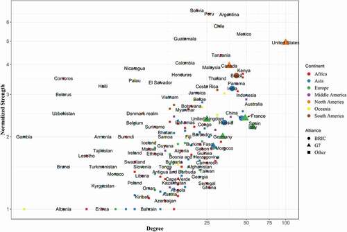
Figure 1 shows the scatterplot of the degree (number of topological neighbors of a node) versus normalized strength (sum of edge weights/degree) for each node in the graph and helps elicit regional trends of ‘research connectivity’. Each node represents a country, colored according to the continent where the country is situated. The shape of each point denotes whether it is in the Group of seven (G7) (Canada, France, Germany, Italy, Japan, the United Kingdom and the US), or Brazil, Russia, India, China (BRIC) grouping. The G7 and BRIC groupings are used to explicitly highlight how economics and politics drives collaborations. Thus, the color and the shape of the points in the plot help reveal spatial and economic trends in ‘research connectivity’. Figure 1 indicates that while a few countries have very high degrees of ‘research connectivity’, led by the US, most countries have low degrees. G7 (mean degree = 47.14, mean normalized strength = 2.8) and BRIC (mean degree = 40.5, mean normalized strength = 2.86) countries have been highlighted to show their relative high degrees and normalized strength (compared to mean degree = 16.7, mean normalized strength = 2.03 of ‘Other’), indicating many strong collaborations formed by their researchers. This indicates that economic factors likely play an important role in forming research connections. Interestingly, there also appears to be regional trends of ‘research connectivity’ between low degree countries. The scatterplot reveals that even though a few countries may only be connected to a few other countries, the ties between them are strong with several grants listing the pairs together. Thus, countries like Tajikistan and Uzbekistan have high normalized strength even though they have low degrees. This is expected as nearby countries often have similar geographic features, and hence are often listed together in grants which study those features. This explains the clustering of the Central Asian countries of Tajikistan, Turkmenistan, and Kyrgyzstan near low degrees but high normalized strength, as well as South and Central American Countries of Bolivia, Argentina, Mexico, Guatemala, and Chile toward high degree and strength.

Figure 1. Scatterplot of Degree versus Normalized Strength in Type 1 network on a log-log graph. Normalized strength is calculated by dividing the sum of the weights of each edge incident on a node by the degree of the node. Each point represents a country where fieldwork was carried out. The BRIC and G7 groupings are shown using different symbols. The color of the points represents the continent

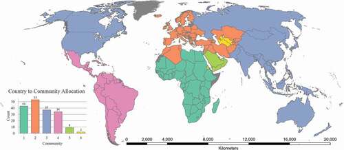
The geographical nodal information is hierarchical in nature as country locations can be grouped into continents, providing a depiction of connectedness at a coarser spatial scale. The aggregated view of the data at the continent level shows that most research takes place within multiple countries in the same continent, but there are grants in which countries in different continents are involved. Figure 2 reveals that there are in fact grants that connect every pair of continents, with North America having the strongest ties to other continents. In terms of SNA, aggregation might be done by looking for nodes in the network that are more densely connected with each other, than to other nodes. Detecting topological communities using the walk trap algorithm (Pons and Latapy 2005) to identify groups of countries with strong collaborations also reveals a similar story. The walk trap algorithm uses the idea of short random walks to find well-connected sub-structures called communities. Since there are few links that connect different topological communities, random walks are more likely to be trapped within the same community. Figure 3 highlights that there is one major topological community spanning North American countries along with a considerable number of Asian, Oceania, and some African countries. This is not surprising considering the high degree centrality of the US. Asian countries share communities with countries from every other continent, while South and Central America belong almost exclusively in Community 4. The homogeneity of topological communities, consisting of multiple countries from the same continent, highlights the dense connections between countries in the same continent. Asian and African countries form several communities because of the large size of the continents, and the large number of countries in these continents. The large number of chords that start and end in Africa and its lack of links to other continents in the chord diagram (Figure 2) is reflected in the bar chart (Figure 3), as the largest community (Community 1) contains only African countries. Interestingly, Community 5 consists of nine countries that are in the Middle East (Bahrain, Oman, Kuwait, Qatar, Saudi Arabia, UAE, and Yemen) and the Horn of Africa (Eritrea and Djibouti), whereas Community 2 consists of countries from Western Asia, Europe, and Morocco. Thus, these communities highlight partially proximate regions. In conclusion, Figures 2 and Figure 3 together explain ‘research connectivity’ in terms of spatial locations and topological connections as expressed through this SSN.

Figure 2. Chord diagram showing fieldwork collaborations across continents in Type 1 network. Each chord in the diagram represents a grant and connects two countries where the fieldwork was carried out. All countries in the same continent are grouped and have the same color

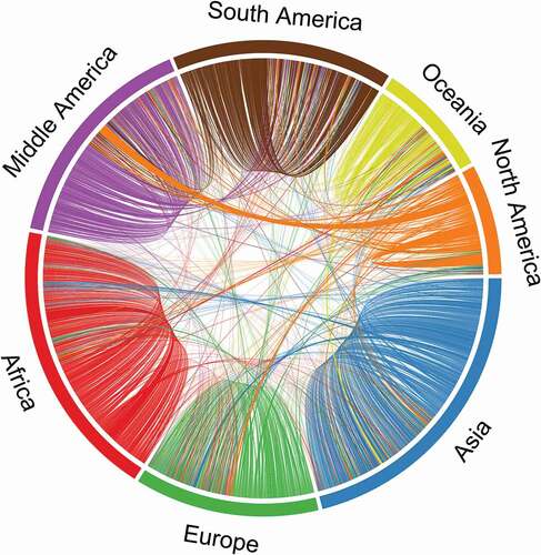
Figure 3. Bar chart showing number of countries in each community detected using the walk-trap algorithm on the Type 1 network along with its map-based representation. The countries denoted in grey do not have community membership associated with them. Given the long 126-year history of the database all the countries represented in the database are not reflected in the map. For example, Serbia and Montenegro was constituted in 1992 and dissolved in 2006. Other countries like Greenland do not appear in the NGS database

4.2. Network 2: how ‘internationalized’ is the research of the various Principal Investigators?

In the second network, both nodes and edges have explicit spatial information. The primary question of interest is: how ‘internationalized’ is the research of the various PIs?

The resulting network is instrumental at predicting possible collaborations between countries based on the patterns of PIs interests in the same field locations. As often reported in literature, in this network too, there is a high correlation between the degree (mean = 25.93, sd = 24.62) and betweenness metrics (mean = 48.03, sd = 181.99) (Valente et al. 2008, Li et al. 2011, 2015). The high variability in the metrics as indicated by the standard deviations implies that some nodes are disproportionately more important topologically. Here, the metrics (and topological importance) correlate with the number of grants that were allocated to PIs from each country. There is disparity in the number of grants obtained by PIs of different countries. PIs from US (70% of all grants), United Kingdom (4% of all grants), and Canada (3% of all grants) account for most number of grants. The correlations imply that these countries are also the ones that have high degree and betweenness. Consequently, it can be inferred that these countries play an important role in keeping the network connected. The number of tenuous connections is high in the database because 46 PI countries and 23 fieldwork locations have only one connection in the 126 years long dataset. Interestingly, despite a high number of tenuous connections because of the single pairings between PI and fieldwork country and the dominance of US in having the greatest number of grants; even if the US is removed, the network remains connected (with 122 nodes and 1473 edges). The mean and standard deviation of degree of nodes drops to 24.15 and 23.12. The mean of betweenness increases to 51.65 while the standard deviation drops to 165.29. The marginal changes in the metrics emphasize that despite the disproportionate influence of the US, the network is highly connected, indicating an ease of forming research collaboration almost anywhere in the world based on common fieldwork locations.

Additionally, instead of just analyzing the country of the PI, countries representing location of the co-applicant of a grant can also be studied. In this case, the nodes represent not only the countries of the PI, but also that of the co-applicants listed in the grants. The grant co-applicants are often researchers from the country where the fieldwork was carried out. Thus, this network highlights the collaborations taking place especially because the research is fieldwork-based. Note that this represents a network that is a superset of the network in which the edges represented only the PI countries. This network consists of 179 nodes representing country of the researcher (PI and co-applicants) and 4426 edges representing the fieldwork countries. The significant increase in the size of this network (number of nodes and edges) compared to the previous network highlights that co-applicants are often from different countries and including them highlights relationships between researcher countries not apparent before.

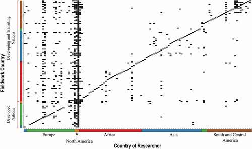
Figure 4 shows a network matrix of researcher’s countries plotted against fieldwork countries grouped together by their World Economic Situation and Prospects (WESP) development status (WESP 2014) and then by continent. This grouping allows exploring economic dimensions and spatial proximity simultaneously. The x-axis and y-axis of the network matrix are symmetrical as they follow the same ordering and grouping of countries. The developed countries are grouped toward the origin of the plot. Japan is the only Asian country marked as developed according to WESP and is plotted closest to the origin of the plot. Along the y-axis (Fieldwork Country), the grouping of countries according WESP development status is made clear by using labels. Along the x-axis (Country of Researcher), the color scheme for continents is explicated with labels. The stark vertical line in the plot represents US, as PIs from US have worked in almost every country (193 out of the 197 fieldwork countries). For countries such as Somalia, Haiti, and Guyana, the potential for collaboration is limited to researchers from US, United Kingdom, and Canada visiting these countries to do research. In fact, for most countries in the database, researchers from developing countries form ties to researchers from developed countries for work in their home countries and/or its neighbors. This is highlighted by the clustering of points along the diagonal for developing countries, implying that for developing countries’ researchers, they either work in their own countries, or in nearby countries. However, PIs from developed countries tend to work everywhere, often in collaboration with co-PIs in the host or nearby countries. This type of collaboration is encouraged by the NGS and this had initially manifested itself in this second network (having both PI and co-applicants) in the form of increased network size.

Figure 4. Network matrix showing the researcher’s country of affiliation along the x-axis and the country where the fieldwork was carried out on the y-axis. The countries are grouped by their WESP development status and then by continents. The order of plotting the countries is the same along the x and y axes with the entries for North America serving as the vertical line separating the developed and the developing nations along the x-axis. The colors denote the continent. The number of entries along the rows and columns of each country gives the degree

4.3. Network 3: what is the multi-disciplinary research potential of different countries?

This network contains spatial information only as part of edges and can be used to explore multi-disciplinary potential of the various countries. The mean and standard deviation of degree of the nodes in this network is 500.43 and 518.47, respectively. The high standard deviation highlights the discrepancy in connectivity or inter-country research efforts put into different fields.

Querying the network for multi-disciplinary research potential achieved in different countries yields interesting results. Despite the great variety of research funded by NGS to researchers from different countries, most of the grants have gone to researchers located in the US. Consequently, research on most combinations of disciplines has been conducted in the US, making the country account for almost 11% of the edges. Further, even though the network is well connected, four nations, namely, US, China, Mexico, and Canada, account for 29% of all the edges, highlighting the predominance and achieved potential for multi-disciplinary research in those countries (19% accounts for G7, and 14% for BRIC countries).

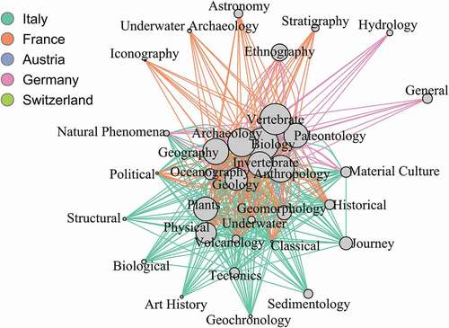
Since the network is created based on grants that have hitherto been given out by NGS, the non-existence of an edge between nodes does not imply that research on those two disciplines is not possible in that country. On the contrary, the missing links potentially points to research opportunities that may yet be untapped or yet to be supported by NGS. For example, among European nations Switzerland is in the bottom 10% of the total number of edges, which suggests low levels of interdisciplinary research. The sparsity of edges representing countries represents an opportunity for more multi-disciplinary research in these countries, especially considering that neighboring countries (i.e., Italy, France, Austria, and Germany) connect 33 disciplines (Figure 5). The core-periphery nature of this graph also highlights which core subject areas NGS grants are focused on (core) and the sub-disciplines that have been explored in each of the countries (periphery). For a well-connected network such as this one, the non-existence of edges is often more interesting than the existence of one. The Switzerland example highlights the potential of using these methods, but also demonstrates the caution required to account for the nature of the dataset. Switzerland hosts several universities and institutes with high research output, and the aforementioned result represents an artifact of this dataset where grants are biased toward US-based researchers.

Figure 5. Graph of neighboring countries of Switzerland highlights potential for research using Network 3. Edges colored according to country. Nodes are sized according to their degrees

Shifting the focus of analysis from the edges to the nodes puts emphasis on the disciplines. Using this network, we can highlight the disciplines that can potentially be researched in only a few countries, if the disciplines are to be explored in conjunction with each other. This implies that an edge (representing a country) must exist between the two disciplines of interest. The degree of the nodes is an indication of the number of countries that can be the field location for research for that discipline. But if one is interested in finding the potential of multi-disciplinary research, it is necessary that an edge links the two nodes. Filtering the network to only keep nodes that have their degrees in the bottom 28% of the degree distribution curve reveals ‘Pollution’ as a theme that can be researched in conjunction with others, such as ‘Freshwater’ and ‘Climate Change’ in both the US and China (Figure 6). The threshold is set at 28% because below this the sub-network contained disconnected components. The sub-network consists of 21 nodes and 91 edges.

Figure 6. Nodes with degrees in the bottom 28% of the degree distribution in the Network 3. Edges are colored according to country. The bold edges show a path connecting ‘Pollution’, ‘Climate Change’, “Innovation and Technology, and ‘Transportation and Communication’ highlighting the potential for a new research topic

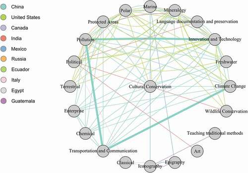
However, this approach of filtering the original network to create a sub-network also produces a significant number of false negatives, that is, combinations of research topics that are likely incompatible (e.g. ‘Marine’ and ‘Terrestrial’). Even in this case, when trying to find a combination for a novel research topic, the absence of edges between node pairs may be more informative than the presence of one. Note that a complementary network (a network with all the edges representing all the countries connecting nodes that are not connected in the primary network) is not created as it would be huge and mostly unhelpful. One may also go beyond selecting just two disciplines and look for longer chains of edges representing the same country to highlight potential research topics, such as, ‘Innovation and Technology’ in ‘Transportation and Communication’ to reduce ‘Pollution’ with the hope of countering ‘Climate Change’ in China (highlighted path in Figure 6). All of the edges in Figure 6 represent weak links due to the nature of network construction. Thus, any potential links need to be examined carefully. ‘Cultural Conservation’ occupies an interesting central position in this network as it seems to bridge the gap between human-centric and environment-centric topics.

5. Discussions

The three networks created in this study incorporate spatial information in different ways. It is important to discuss what is shown in these network structures, how they compare to network realizations used in GIScience; and what insights the analysis provides. Network 1, with edges depicting countries where the fieldwork was carried out and the edges represent grants, is the most common representation of spatial social networks where the spatial information is part of the nodes. However, the location anchored sociogram representation of such a large graph would produce a hairball-like structure with little visually discernable information. Instead, regional patterns of fieldwork locations are elicited by resorting to alternate visualizations. Further, Network 1 are probably the easiest to conceptualize and even by using this method with the NGS database, several different networks could have been made. For example, the nodes could have represented the countries of the connected researchers, if the same grant had co-PIs from two countries. However, such a network is similar to co-authorship networks and would not facilitate exploring the unique possibilities of using fieldwork locations as a collaboration opportunity offered by this database. Because of the nature of research supported by NGS, the network created is able to highlight interesting regional trends about fieldwork-based research collaboration (Figures 3.1 and 3.2).

Network 2, when compared to a citation or co-authorship-based network, displays similarities because in both cases the primary emphasis is on first-degree connections. In a citation network, existence of a path between two nodes may imply that the two papers are in similar, but not necessarily in the same field. However, the connected nature of the network highlights the linked interdisciplinary nature of science (Börner et al. 2003, Boyack et al. 2005, Leydesdorff and Schank 2008, Porter and Rafols 2009). Similarly, this network highlights that researchers in different countries may be interested in the same fieldwork location even if they are not working on the same topics, and consequently portrays the highly connected nature of fieldwork-based research. Unlike a citation-based network, the resolution at which this network was created makes it of limited use to understand potential collaborations beyond the first degree. Creating a finer resolution version of this network may emphasize interests among researchers in specific domains working in particular field sites and consequently highlight potential future collaborations.

In Network 3, spatial information is associated with the edges but not with nodes. This conceptualization of network spatiality is feasible only in case of social networks where the edges represent conceptual connections. In case of physical networks like roads, the physicality of the edges also enforces spatiality on the nodes. Similar co-editing networks have been created from OpenStreetMap where two users are connected if they edited the same spatial object (Mooney and Corcoran 2014). Liberating the spatiality constraints from the nodes enables the edges to be free from having length as one of the attributes, a necessary condition in case of road networks. Having a network-based conceptualization where the nodes represent grant disciplines that are inherently non-spatial is difficult to represent in GISystem. The closest analogy in a GISystem would be to add the disciplines researched in each country as attribute information, and resort to attribute-based queries to highlight combinations of disciplines researched in various countries. Such a GISystem based model requires significant data manipulation to focus on the connections between various disciplines, especially when creating larger chains of country discipline pairings to suggest potential research collaborations (Figure 3.6 highlighted path). GISystem based representation, while not ideally suitable for ‘connectivity’ based analysis, is better suited to reveal spatial patterns in disciplinary research. Note that for the Network 3, an alternate configuration could have been made with the nodes representing the fieldwork location, and the edges representing the disciplines. This would have been akin to the Network 1 as to how spatial information is incorporated. In this alternate configuration, the focus shifts to the fieldwork countries rather than the disciplines. The questions that can be asked of this configuration are quite different. For example, what are the common topics of research between two countries, rather than asking which research topics can be explored together in a country. Even though questions pertaining to both the actual Network 3 and the alternate configuration can be asked of both network conceptualizations with sufficient data processing, each network configuration is better suited to addressing a particular question. This further highlights the flexibility of the network structure in modeling plurality of relationships latent in a dataset.

There are limitations specific to the NGS dataset used as a case-study here. Given the long-time frame of the grants database, country details (e.g., names, physical boundaries) have changed over time. In this study, the names as recorded in the database are maintained. Most grants have country-level reporting with no distinction between locations within the same country. This is particularly an issue for large countries like the US. In addition, although this database is remarkable for its geographical coverage, NGS being a US-based organization has over-representation of its home country. Whereas this database provides an interesting look at collaborations; it does not equally represent all countries. Nevertheless, the results revealed a global pattern of scientific collaborations and the increasing efforts of granting organizations to diversify research both in terms of disciplines and demographics. It is worth reiterating that the primary aim of this paper is to emphasize the various ways of creating SSNs by using the NGS database as a case study. Thus, generalization of these results requires careful deliberation. Supplementing this dataset with other datasets as well as other forms of analysis, which include enriching the nodes and edges with additional attribute information along with complimentary co-authorship and citation-based studies, should provide a more generalizable and concrete picture of global collaborations.

6. Conclusion

Here, an innovative use of SSN methods and visualization techniques to emphasize the potential for answering varied geographic questions related to International research collaborations from the NGS’s grants database is highlighted. Further, the many forms of representation by which spatial information can be incorporated into the node and edge structure is emphasized. These altered perspectives yield unique insights on the nature of the spatial social network, and consequently can be applied to most standard databases with spatial identifiers.

The varied network conceptualizations of the same database capture geographic information differently and provide insights into the myriad spatial perspectives latent in a dataset. Thus, the analysis demonstrates the usefulness of these methods at providing insights into systems in which spatial information is a crucial enabler of relationships. Similar approaches may be used on a variety of different systems in which relationships and spatial information are integral for understanding the system. Each network representation answers a different question. Thus, the multitude of networks created from this one dataset gave insights on structure of collaborations that have been reported in literature. For example, Network 1 indicated that few countries have a high degree of research connectivity and there are significant regional trends. This is akin to previous research presented by Adams et al. (2014), who identified that collaborations patterns in Africa were far from universal; instead they were affected by regional geographic factors such as history, culture, and language. Similar homogeneity in collaborative research was also reported in the field of Ecology where geographic distance and socioeconomic factors were a determining factors for highly collaborative countries (Parreira et al. 2017). Network 2 identified that international research often means collaborating with local researchers. This is contrary to the distance decay in scientific networks of patent co-applicants noted among Organisation for Economic Co-operation and Development (OECD) countries (Cerina et al. 2014). Due to the nature of grants supported by NGS, there are a significant number of cross-boundary collaboration. However, researchers from developed countries work everywhere, whereas researchers from developing countries work mostly in their own countries or in nearby countries. Binka (2005) terms this ‘scientific colonialism’, although there are welcome signs of concentrated efforts by researchers and granting agencies to turn these into more equitable partnerships (Atickem et al. 2019). In this dataset too, despite NGS being a United States based organization, over the years there has been efforts to diversify grant recipients as evidenced by the high resilience of the Network 2 to disconnection. Analyzing Network 3 helped in understanding and identifying potential for interdisciplinary research in different countries, which has been shown to lead to a convergence between applied and theoretical fields supporting the evolution of scientific disciplines (Coccia and Wang 2016).

New ideas and techniques of using SSNs to analyze large, spatially explicit datasets and use a grants database as a case-study are presented here. The analyses allowed new interpretations of collaborations and collaborative potential. The nature of research supported by the NGS implies that considerable fieldwork is involved, which engenders various forms of interaction opportunities between researchers of various countries. These interactions create opportunities for collaborations which may not be evident using a standard SNA analysis carried out on a database of citations and co-authorship. Hence, varied conceptualizations of a spatially explicit database as SSNs can yield interesting insights regarding spatial relationships that may not be apparent by using other spatial analysis techniques.

Acknowledgments

We would like to thank Dr. Peter Raven and the team at National Geographic Society for giving us access to the dataset.

Data and code availability statement

The data used for the analysis belongs to National Geographic Society, and therefore a mock dataset is provided. The primary aim of this article is to demonstrate that various spatially explicit networks can be created from the same dataset. Please visit https://doi.org/10.5281/zenodo.3689782 for the mock data shown in Table 3A and the associated code to produce the networks illustrated in Table 3B, C, and D.

Disclosure statement

No potential conflict of interest was reported by the author(s).

Additional information

Notes on contributors

Dipto Sarkar

Dipto Sarkar is an Assistant Professor in the Department of Geography and Environmental Studies at Carleton University. His research focuses on geographic information science, social networks, and computational social sciences. He is particularly interested in applying his methods to understand the human dimensions of biodiversity conservation.

Colin A. Chapman

Colin A. Chapman’s research focuses on how the environment influences animal abundance and social organization and given their plight, he has applied his research to primate conservation. Colin Chapman received his joint Ph.D. in the Departments of Anthropology and Zoology at the University of Alberta. He spent 2 years at McGill and 3 years at Harvard University doing post-doctoral research. Since 1990 he has served as an Honourary lecturer in the Department of Zoology at Makerere University, Uganda and since 1995 he has been a Conservation Fellow with the Wildlife Conservation Society. Colin also served as a faculty member in Zoology at the University of Florida for 11 years and returned to McGill in 2004 where he held a Canada Research Chair Tier 1 position in Primate Ecology and Conservation. He is a Killam Research Fellow, Velan Foundation Awardee for Humanitarian Service, and is a fellow of the Royal Society of Canada. In 2018 he was awarded the Konrad Adenauer Research Award from the Alexander von Humboldt Foundation and an Office of an Academician, Northwest University, Xi’an, China. In 2019 he took up a position at George Washington University to allow him to more time for his conservation efforts. For the last 30+ years, Dr. Chapman has conducted research in Kibale National Park, Uganda. During this time, he has not just been an academic, but has devoted great effort to help the rural communities, establishing schools, clinics, a mobile clinic, and ecotourism projects. He has published 520+ articles, been cited 40000+ times, has a H factor of 104 (Google Scholar) and has received ~ $21 million in funding.

Raja Sengupta

Raja Sengupta is an Associate Professor in the Department of Geography and School of Environment at McGill University, Montreal, Quebec, Canada. His research interests are centered around various GIScience topics, including Agent-Based Models (ABMs) of both human and primates. He is also interested to understand how resource sites can be locations for transmissions of infectious diseases (as verified using ABMs), and is using network analysis to understand both spread of diseases and landscape-based factors that affect movement patterns of primates and other animals. He has published 41 journal papers, 10 book chapters, and one edited volume on related topics. He is also active as Scientific Committee member of several GIScience related conference series (e.g., GIScience, Spatial Knowledge and Information Canada).

References

- Abizaid, C., et al., 2015. Social network analysis of peasant agriculture: cooperative labor as gendered relational networks. The Professional Geographer, (March), 1–17. https://doi.org/https://doi.org/10.1080/00330124.2015.1006562
- Abizaid, C., Coomes, O.T., and Perrault-Archambault, M., 2016. Seed sharing in amazonian indigenous rain forest communities: a social network analysis in three Achuar Villages, Peru. Human Ecology, 44, 577–594. doi:https://doi.org/10.1007/s10745-016-9852-7
- Adams, J., 2013. The fourth age of research. Nature, 497 (7451), 557–560. doi:https://doi.org/10.1038/497557a.
- Adams, J., et al., 2014. International collaboration clusters in Africa. Scientometrics, 98 (1), 547–556. doi:https://doi.org/10.1007/s11192-013-1060-2.
- Alfano, M., et al., 2018. Social network-epistemology. In: 2018 IEEE 14th International Conference on e-Science (e-Science). Presented at the 2018 IEEE 14th International Conference on e-Science (e-Science), Amsterdam, Netherlands. 320–321.
- Andris, C., 2016. Integrating social network data into GISystems. International Journal of Geographical Information Science, 8816 (March), 1–23. doi:https://doi.org/10.1080/13658816.2016.1153103.
- Andris, C., Liu, X., and Ferreira, J., 2018. Challenges for social flows. Computers, Environment and Urban Systems, 70 (October 2017), 197–207. doi:https://doi.org/10.1016/j.compenvurbsys.2018.03.008.
- Atickem, A., et al., 2019. Build science in Africa. Nature, 570 (7761), 297–300.
- Barthélemy, M., 2011. Spatial networks. Physics Reports, 499 (1–3), 1–101. doi:https://doi.org/10.1016/j.physrep.2010.11.002.
- Batty, M., 2003. The geography of scientific citation. Environment and Planning A: Economy and Space, 35 (5), 761–765. doi:https://doi.org/10.1068/a3505com.
- Binka, F., 2005. Editorial: north-South research collaborations: a move towards a true partnership? Tropical Medicine and International Health, 10 (3), 207–209. doi:https://doi.org/10.1111/j.1365-3156.2004.01373.x.
- Börner, K., Chen, C., and Boyack, K.W., 2003. Visualizing knowledge domains. Annual Review of Information Science and Technology, 37 (1), 179–255. doi:https://doi.org/10.1002/aris.1440370106.
- Boyack, K.W., Klavans, R., and Börner, K., 2005. Mapping the backbone of science. Scientometrics, 64 (3), 351–374. doi:https://doi.org/10.1007/s11192-005-0255-6.
- Buch-Hansen, H., 2014. Social network analysis and critical realism. Journal for the Theory of Social Behaviour, 44 (3), 306–325. doi:https://doi.org/10.1111/jtsb.12044.
- Castells, M., 1996. The rise of the network society. Oxford: Blackwell.
- Cerina, F., et al., 2014. Network communities within and across borders. Sci Rep 4, 4546. https://doi.org/https://doi.org/10.1038/srep04546
- Coccia, M. and Wang, L., 2016. Evolution and convergence of the patterns of international scientific collaboration. Proceedings of the National Academy of Sciences, 113 (8), 2057–2061. doi:https://doi.org/10.1073/pnas.1510820113.
- Derudder, B., et al., 2013. Measurement and interpretation of connectivity of Chinese cities in world city network, 2010. Chinese Geographical Science, 23 (3), 261–273. doi:https://doi.org/10.1007/s11769-013-0604-y.
- Derudder, B. and Liu, X., 2016. How international is the annual meeting of the Association of American Geographers? A social network analysis perspective. Environment and Planning A, 48 (2), 309–329. doi:https://doi.org/10.1177/0308518X15611892.
- Egenhofer, M.J. and Franzosa, R.D., 1991. Point-set topological spatial relations. International Journal of Geographical Information Systems, 5 (2), 161–174. doi:https://doi.org/10.1080/02693799108927841.
- Emch, M., et al., 2012. Integration of spatial and social network analysis in disease transmission studies. Annals of the Association of American Geographers. Association of American Geographers, 105 (5), 1004–1015. doi:https://doi.org/10.1080/00045608.2012.671129.
- Entwisle, B., Rindfuss, R.R., and Faust, K., 2007. Networks and contexts : variation in the structure of social ties 1. American Journal of Sociology, 112 (5), 1495–1533. doi:https://doi.org/10.1086/511803.
- Faust, K., et al., 2000. Spatial arrangement of social and economic networks among villages in Nang Rong District, Thailand. Social Networks, 21 (4), 311–337. doi:https://doi.org/10.1016/S0378-8733(99)00014-3.
- Fleming, L. and Sorenson, O., 2001. Technology as a complex adaptive system: evidence from patent data. Research Policy, 30 (7), 1019–1039.
- Giebultowicz, S., et al., 2011a. The simultaneous effects of spatial and social networks on cholera transmission. Interdisciplinary Perspectives on Infectious Diseases, 2011, 604372. doi:https://doi.org/10.1155/2011/604372
- Giebultowicz, S., et al., 2011b. A comparison of spatial and social clustering of cholera in Matlab, Bangladesh. Health & Place, 17 (2), 490–497. doi:https://doi.org/10.1016/j.healthplace.2010.12.004.
- Hou, H., Kretschmer, H., and Liu, Z., 2008. The structure of scientific collaboration networks in Scientometrics. Scientometrics, 75 (2), 189–202. doi:https://doi.org/10.1007/s11192-007-1771-3.
- Jiang, B., 2007. A topological pattern of urban street networks: universality and peculiarity. Physica A: Statistical Mechanics and Its Applications, 384 (2), 647–655. doi:https://doi.org/10.1016/j.physa.2007.05.064.
- Kadushin, C., 2012. Understanding social networks. Oxford: Oxford University Press.
- Keeling, M.J., et al., 2011. Networks and the epidemiology of infectious disease. Interdisciplinary Perspectives on Infectious Diseases, 2011. https://doi.org/https://doi.org/10.1155/2011/284909
- Kretschmer, H., 1997. Patterns of behaviour in coauthorship networks of invisible colleges. Scientometrics, 40 (3), 579–591. doi:https://doi.org/10.1007/BF02459302.
- Kretschmer, H., 2004. Author productivity and geodesic distance in bibliographic co-authorship networks, and visibility on the Web. Scientometrics, 60 (3), 409–420. doi:https://doi.org/10.1023/B:SCIE.0000034383.86665.22.
- Leydesdorff, L. and Schank, T., 2008. Dynamic animations of journal maps: indicators of structural changes and interdisciplinary developments. Journal of the American Society for Information Science and Technology, 59 (11), 1810–1818. doi:https://doi.org/10.1002/asi.20891.
- Leydesdorff, L., Wagner, C.S., and Bornmann, L., 2018. Betweenness and diversity in journal citation networks as measures of interdisciplinarity—A tribute to Eugene Garfield. Scientometrics, 114 (2), 567–592. doi:https://doi.org/10.1007/s11192-017-2528-2.
- Li, C., et al., 2011. The correlation of metrics in complex networks with applications in functional brain networks. Journal of Statistical Mechanics: Theory and Experiment, 2011 (11), P11018. doi:https://doi.org/10.1088/1742-5468/2011/11/P11018.
- Li, C., et al., 2015. Correlation between centrality metrics and their application to the opinion model. The European Physical Journal B, 88 (3), 1–13. doi:https://doi.org/10.1140/epjb/e2015-50671-y.
- Liben-Nowell, D., et al., 2005. Geographic routing in social networks. Proceedings of the National Academy of Sciences of the United States of America, 102 (33), 11623–11628. doi:https://doi.org/10.1073/pnas.0503018102.
- Liu, X. and Derudder, B., 2012. Two‐mode networks and the interlocking world city network model: a reply to neal. Geographical Analysis, 44 (2), 171–173. doi:https://doi.org/10.1111/j.1538-4632.2012.00844.x.
- Liu, X. and Derudder, B., 2013. Analyzing urban networks through the lens of corporate networks: a critical review. CITIES, 31, 430–437. doi:https://doi.org/10.1016/j.cities.2012.07.009
- Mao, L., 2014. The geography, structure, and evolution of the GIS research community in the US: A network analysis from 1992 to 2011. Transactions in GIS, 18 (5), 704–717. doi:https://doi.org/10.1111/tgis.12054.
- McPherson, M., Smith-Lovin, L., and Cook, J.M., 2001. Birds of a feather: homophily in social networks. Annual Review of Sociology, 27, 415–444. doi:https://doi.org/10.1146/annurev.soc.27.1.415
- Mooney, P., and Corcoran, P., 2014. Analysis of interaction and co-editing patterns amongst openstreetmap contributors. Transactions in GIS, 18 (5), 633–659.
- Mossa, S., et al., 2005. The worldwide air transportation network: anomalous centrality, community structure, and cities’ global roles. Proceedings of the National Academy of Sciences of the United States of America, 102 (22), 7794–7799. doi:https://doi.org/10.1073/pnas.0407994102.
- Otte, E. and Rousseau, R., 2002. Social network analysis: a powerful strategy, also for the information sciences. Journal of Information Science, 28 (6), 441–453. doi:https://doi.org/10.1177/016555150202800601.
- Owen-Smith, J. and Powell, W.W., 2004. Knowledge networks as channels and conduits: the effects of spillovers in the boston biotechnology community. Organization Science, 15 (1), 5–21. doi:https://doi.org/10.1287/orsc.1030.0054.
- Parreira, M.R., et al., 2017. The roles of geographic distance and socioeconomic factors on international collaboration among ecologists. Scientometrics, 113 (3), 1539–1550.
- Pons, P. and Latapy, M., 2005. Computing communities in large networks using random walks. In: Yolum., T. Güngör, F. Gürgen, C. Özturan, eds. Computer and Information Sciences - ISCIS 2005. Lecture Notes in Computer Science. Berlin, Heidelberg: Springer. https://doi.org/https://doi.org/10.1007/11569596_31
- Porta, S., Crucitti, P., and Latora, V., 2006. The network analysis of urban streets: A dual approach. Physica A: Statistical Mechanics and Its Applications, 369 (2), 853–866. doi:https://doi.org/10.1016/j.physa.2005.12.063.
- Porter, A.L. and Rafols, I., 2009. Is science becoming more interdisciplinary? Measuring and mapping six research fields over time. Scientometrics, 81 (3), 719–745. doi:https://doi.org/10.1007/s11192-008-2197-2.
- Preciado, P., et al., 2011. Does proximity matter? Distance dependence of adolescent friendships. Social Networks, 34 (1), 18–31.
- Prell, C., 2012. Social network analysis. London: SAGE Publications Ltd.
- Radil, S.M., Flint, C., and Tita, G.E., 2010. Spatializing social networks: using social network analysis to investigate geographies of gang rivalry, territoriality, and violence in Los Angeles. Annals of the Association of American Geographers, 100 (2), 307–326. doi:https://doi.org/10.1080/00045600903550428.
- Sarkar, D., Sieber, R., and Sengupta, R., 2016. GIScience considerations in spatial social networks. In: J.A. Miller, D.O. Sullivan, and N. Wiegand, eds. Lecture notes in computer science. 85–98. Springer International Publishing.
- Sarkar, D., et al., 2019. Metrics for characterizing network structure and node importance in spatial social networks. International Journal of Geographical Information Science, 33 (5), 1017–1039. doi:https://doi.org/10.1080/13658816.2019.1567736.
- Scellato, S., et al., 2011. Socio-spatial properties of online location-based social networks. Proceedings of the International AAAI Conference on Web and Social Media. Available from https://ojs.aaai.org/index.php/ICWSM/article/download/14094/13943
- Sun, S. and Manson, S.M., 2011. Social network analysis of the academic GIScience community. The Professional Geographer, 63 (1), 18–33. doi:https://doi.org/10.1080/00330124.2010.533560.
- Valente, T.W., et al., 2008. How correlated are network centrality measures? Connections, 28 (1), 16–26.
- Wagner, C.S. and Leydesdorff, L., 2005. Network structure, self-organization, and the growth of international collaboration in science. Research Policy, 34 (10), 1608–1618. doi:https://doi.org/10.1016/j.respol.2005.08.002.
- Wagner, C.S., Park, H.W., and Leydesdorff, L., 2015. The Continuing Growth of Global Cooperation Networks in Research: A Conundrum for National Governments. PLOS ONE, 10 (7), e0131816.
- WESP, 2014. Country classification system. Available from https://www.un.org/en/development/desa/policy/wesp/wesp_current/2014wesp_country_classification.pdf
- Wong, L.H., Pattison, P., and Robins, G., 2006. A spatial model for social networks. Physica A: Statistical Mechanics and Its Applications, 360 (1), 99–120. doi:https://doi.org/10.1016/j.physa.2005.04.029.
- Ye, X. and Liu, X., 2018. Integrating social networks and spatial analyses of the built environment. Environment and Planning B: Urban Analytics and City Science, 45 (3), 395–399.
- Zhong, C., et al., 2014. Detecting the dynamics of urban structure through spatial network analysis. International Journal of Geographical Information Science, 28 (11), 2178–2199. doi:https://doi.org/10.1080/13658816.2014.914521.
- Zuckerman, E.W., 2008. Why social networks are overrated (a 3+ when they are at best a 2) [online]. OrgTheory.net. Available from: http://orgtheory.wordpress.com/2008/11/14/why-social-networks-are-overrated-a-3-when-they-are-at-best-a–2/