Geographically and temporally weighted co-location quotient: an analysis of spatiotemporal crime patterns in greater Manchester

Abstract

Incident data, a form of big data frequently used in urban studies, are characterized by point features with high spatial and temporal resolution and categorical values. In contrast to panel data, such spatial data pooled over time reflect multi-directional spatial effects but only unidirectional temporal effects, which are challenging to analyze. This paper presents an innovative approach to address this challenge – a geographically and temporally weighted co-location quotient which includes global and local computation, a method to calculate a spatiotemporal weight matrix and a significance test using Monte Carlo simulation. This new approach is used to identify spatio-temporal crime patterns across Greater Manchester in 2016 from open source recorded crime data. The results show that this approach is suitable for the analysis and visualization of spatio-temporal dependence and heterogeneity in categorical spatial data pooled over time. It is particularly useful for detecting symmetrical spatio-temporal co-location patterns and mapping local clusters. The method also addresses the unbalanced temporal scale problem caused by unidirectional temporal data representation and explores potential impacts. The empirical evidence of the spatiotemporal crime patterns might usefully be deployed to inform the development of criminological theory by helping to disentangle the relationships between crime and the urban environment.

Keywords:

• Spatial data pooled over time
• unbalanced temporal scale problem
• geographically and temporally weighted co-location quotient
• spatiotemporal crime patterns
• open recorded data

1. Introduction

Rapid advances in remote sensing and computer technology, since the inception of GIS, have led to a significant evolution in urban GIS analyses and data, from land use and land cover modelling using satellite imagery, to the analysis of spatial accessibility by integrating spatial and socio-economic census data, and to mobility and sentiment analysis using newly available big data and open data. Although there is no standard definition of big data, it is typically characterized by the 3Vs – the dimensions of volume, variety and velocity – and sometimes a further 6Vs (veracity, validity, variability, volatility, visualization and value) (Batty and Michael 2016). Among these Vs, high velocity indicates that data are generated through a streaming process in real time and in a continuous fashion, rather than batch processing. High velocity enables the production of data with high temporal resolution, particularly suitable for modelling urban dynamics. Driven by a variety of factors including citizen science, big data is increasingly used in urban studies to analyze rapid changes in population and associated socio-economic activity (Kharrazi et al. 2016, Bannister and O'Sullivan 2021). Data infrastructure developments have driven the emergence of urban analytics (Liu et al. 2020, Kandt and Batty 2021) which, for example, has been used to analyze crime patterns from a variety of big and small data sets (Helbich and Leitner 2017, Zahnow and Corcoran 2021).

Geographically weighted spatial modeling (GWSM) is commonly used in urban and geographical studies due to its suitability for exploring spatial nonstationarity and mapping local relationships. Since the publication of the seminal book on geographically weighted regression (GWR) in 2002 (Fotheringham et al. 2002), GWSM has been continuously developed to include semi-parametric or mixed GWR (Nakaya et al. 2005), geographically (or spatially) and temporally weighted regression (GTWR) (Huang et al. 2010, Fotheringham et al. 2015), multi-scale GWR (Fotheringham and Oshan 2016) and multi-scale GTWR (Wu et al. 2018). GTWR is able to quantify and visualize the spatial and temporal processes underlying complicated geographical patterns (e.g., the dynamics of house prices). Another parallel development in GWSM has been the spatial extension of traditional statistical or mathematical methods, such as geographically weighted principal component analysis (Harris et al. 2015, Li et al. 2016), geographically weighted flow modelling (Zhang et al. 2019) and, geographically weighted co-location quotient analysis (Cromley et al. 2014). The co-location quotient, developed from the traditional economic geography location quotient, has been increasingly used to measure the directed spatial dependence between categorical variables. Many types of urban big data are categorical variables, such as POI data that have location and nominal attribute values but no numerical values (e.g., interval or ratio). Location quotient is a popular method for measuring regional specialization in economic geography, but it is subject to the modifiable areal unit problem (MAUP) ( Eckardt and Mateu 2021). The co-location quotient (CLQ) aims to quantify the spatial association between categories of a population that may exhibit spatial autocorrelation. It can also detect symmetry and asymmetry in spatial dependence (Cao et al. 2017). Cromley et al. (2014) extended the global CLQ to a geographically weighted co-location quotient (GWCLQ) that takes into account the spatial heterogeneity of the association between categorical data. Wang et al. (2017) further improved the method by proposing a statistical significance test for the derived GWCLQ. All these methodological developments have enabled the incorporation of GWCLQ into ArcGIS Pro 2.8.

In urban crime analytics, the co-location quotient method has been used to analyze geographical patterns. Co-location patterns in criminology can be classified into three categories: co-location between crime types (Pope and Song 2015); co-location between crime types and facilities (e.g., alcohol outlets) (Wang et al. 2017); and co-location between crime incidence sites and the surrounding land use features (Yue et al. 2017). These empirical studies have revealed co-location patterns in crime via global (Pope and Song 2015) or local versions of GWCLQ (Cromley et al. 2014, Wang et al. 2017). However, these analyses only considered spatial dependence and spatial heterogeneity. The benefits of simultaneously incorporating spatial and temporal dimensions in the study of crime patterns have been demonstrated in recent studies spanning: near repeat analysis (Piza and Carter 2018); temporal typology of crimes (Corcoran et al. 2021); crime prediction (Jefferson 2018); seasonal crime trends (Quick et al. 2019); and, spatio-temporal methods for crime prediction (Yang et al. 2020).

Against this backdrop, this paper presents an innovative method of geographically and temporally weighted co-location quotient analysis (GTWCLQ) which, incorporates spatial and temporal dimensions as well as addressing the unbalanced temporal scale problem. The method is validated in a case study of spatiotemporal crime patterns in Greater Manchester. In the rest of this paper, Section 2 describes the data set and analytical method of GTWCLQ. Section 3 presents the GTWCLQ results and interprets the spatio-temporal patterns of crime. Section 4 discusses the outstanding methodological and technical issues and proposes some solutions, and section 5 ends with conclusions and recommendations for future work.

2. Data and methods

This section summaries the key characteristics of the spatio-temporal data used, and explains the development of the GTWCLQ.

2.1. Spatio-temporal data

With the advances in information communications technology (ICT) and the subsequent proliferation of smart cities, large volumes of spatio-temporal data have been generated comprising specific geographic locations and corresponding time stamps (Emani et al. 2015, Wang et al. 2020a). Evaluating patterns and processes in spatial-temporal data has relevance in urban analytics (Kandt and Batty 2021) and urban studies (Bannister and O'Sullivan 2021), as well as in other disciplines including climate science, neuroscience, social sciences, epidemiology, transportation, and earth sciences (Vega-Oliveros et al. 2019, Ferreira et al. 2020).

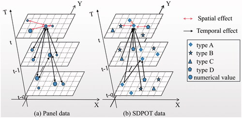
Multiple formats of spatio-temporal data have been used in urban studies (e.g., geo-referenced time series, event data and trajectory data) (Ansari et al. 2019, Atluri et al. 2019). Spatio-temporal panel data and spatial data pooled over time (SDPOT) (Dubé and Legros 2013) are the most common formats of event or incident point data. As shown in Figure 1, panel data are repeat measurements at fixed locations and regular time intervals (e.g., hourly air quality monitoring at fixed stations) but SDPOT are spatially and temporally random incidents (e.g., traffic incidents). Panel data are typically recorded as numerical values, intervals or ratios, whereas SDPOT data are recorded as nominal or ordinal values (such as crime type and accident severity).

Figure 1. Comparison between traditional panel data and SDPOT data: (a) panel data with numerical values at fix location (b) SDPOT data with categorical values at random location.

In terms of data modelling, both panel and SDPOT data are typically represented by a three-dimensional coordinate system (X, Y, T), where X and Y are latitude and longitude in a geographic coordinate system or a locally projected system (e.g., the British national grid system), and T indicates the time of data reporting or collection. In contrast to panel data, the temporal effect in SDPOT is unidirectional because events occurring yesterday will influence today’s pattern but not vice versa. Its spatial effect is multidirectional within the same time period. These features point to the unbalanced temporal scale problem (UTSP) associated with SDPOT data analysis, in that data may represent different temporal durations. For example, in the analysis of monthly crime data over the period of one year, 12 months of data will be available for the pattern analysis of crimes in month 12 (December) but only 6 months of data will be available in month 6 (June) and only 1 month of data will be available in month 1 (January). In other words, there is an unbalanced sample size in spatio-temporal analysis between time points, as the temporal scale (duration) increases at each time point throughout the year. As with classical spatial panel data analysis, the analysis of SDPOT data should account for spatio-temporal dependence and heterogeneity (Tobler 1970).

2.2. Geographically and temporally weighted colocation quotient

Two key methods have sought to incorporate the temporal dimension into geographically weighted modelling, in order to capture both spatial and temporal heterogeneity (Lee and Li 2017, Wang and Lam 2020). The first method combines spatial and temporal effects using a three-dimensional coordinate system (X, Y, T) and introduces two scale parameters to adjust for spatial and temporal effects (Wang et al. 2017). This method is widely used in geographically and temporally weighted regression models. The second method constructs the spatial and temporal weight matrices separately and combine them into a spatio-temporal weight matrix using a Kronecker/Hadamard product (Dubé and Legros 2015). Here, the last one was used to constructs the spatio-temporal weight matrix. In the following descriptions, it is supposed that GTWCLQ targets the spatio-temporal pattern at time t (actual or observational time point). All the points at previous times will be used for global and local computations based on a spatial and temporal distance decay effect.

The basic structure of a global geographically weighted CLQ is defined as: (1) $$\mathit{GWCL}{Q}_{A-B}^g=\frac{\sum _{i\in C}\sum _{j\in D(i\ne j)}{W}_{ij}{x}_j}{M\sum _{i\in C}\sum _{j\in D(i\ne j)}{W}_{ij}}$$(1) (2) $$M=\frac{N_B}{N-1}$$(2) where ${\mathrm{GWCLQ}}_{\mathrm{A}-\mathrm{B}}^{\mathrm{g}}$ is the global geographically weighted colocation quotient for type A relative to type B; ${\mathrm{W}}_{\mathrm{ij}}\mathrm{ }$ denotes the spatial weight matrix, ${\mathrm{x}}_{\mathrm{ij}}$ is a binary variable that equals 1 if the jth point is a marked B-point and is equal to 0 otherwise. $\mathrm{N}$ is the total number of sample and ${\mathrm{N}}_{\mathrm{B}}$ are the number of category B.

By incorporating the temporal distance between two observations, ${\mathrm{GWCLQ}}_{\mathrm{A}-\mathrm{B}}^{\mathrm{g}}\mathrm{ }$ is modified to ${\mathrm{GTWCLQ}}_{\mathrm{A}-\mathrm{B}}^{\mathrm{g}}\mathrm{ }$(global geographically and temporally weighted co-location quotient), which is formulated as follows (Equation 3(3) $$\begin{array}{c}G\mathit{TWCL}{Q}_{A-B}^g=\frac{\sum _{k\in E}\sum _{i\in C}\sum _{j\in D_k}{W}_{ij}{t}_k{x}_{kj}}{M\sum _{k\in E}\sum _{i\in C}\sum _{j\in D_k}{W}_{ij}{t}_k}\\ \end{array}$$(3) ): (3) $$\begin{array}{c}G\mathit{TWCL}{Q}_{A-B}^g=\frac{\sum _{k\in E}\sum _{i\in C}\sum _{j\in D_k}{W}_{ij}{t}_k{x}_{kj}}{M\sum _{k\in E}\sum _{i\in C}\sum _{j\in D_k}{W}_{ij}{t}_k}\\ \end{array}$$(3)

Let $W_{\mathit{ijk}}=W_{ij}{t}_k,$ then ${\mathrm{GTWCLQ}}_{\mathrm{A}-\mathrm{B}}^{\mathrm{g}}\mathrm{ }$ can be modified to Equation 4(4) $$\mathit{GTWCL}{Q}_{A-B}^g=\frac{\sum _{k\in E}\sum _{i\in C}\sum _{j\in D_k}{W}_{\mathit{ijk}}{x}_{kj}}{M\sum _{k\in E}\sum _{i\in C}\sum _{j\in D_k}{W}_{\mathit{ijk}}}$$(4) : (4) $$\mathit{GTWCL}{Q}_{A-B}^g=\frac{\sum _{k\in E}\sum _{i\in C}\sum _{j\in D_k}{W}_{\mathit{ijk}}{x}_{kj}}{M\sum _{k\in E}\sum _{i\in C}\sum _{j\in D_k}{W}_{\mathit{ijk}}}$$(4) where ${\text{ GTWCLQ}}_{\mathrm{A}-\mathrm{B}}^{\mathrm{g}}\mathrm{ }$ denotes the global geographically and temporally weighted co-location quotient of type A relative to type B at time k. $W_{\mathit{ijk}}$ is a spatio-temporal weight denoting the relative importance of the jth point at time k to the ith A-point at actual time. $x_{kj}$ is a binary value that equals 1 if the jth point at time k is a type B point, and is equal to 0 otherwise. E is the set of time periods in study. C is the set of type A points at actual time and $D_k$ is the set of all points at time k. Values greater than one show that type A points tend to be spatially dependent on type B points at time k, while values less than one indicate that type A points are likely to be far from type B at time k. The larger the value, the stronger the dependence or attraction. Asymmetry is defined by the condition that only one of ${\mathrm{GTWCLQ}}_{\mathrm{A}-\mathrm{B}}^{\mathrm{g}}$ and ${\mathrm{GTWCLQ}}_{\mathrm{B}-\mathrm{A}}^{\mathrm{g}}$ is greater than 1 at a 5% significance or lower level.

It is noteworthy that, $\mathrm{N}$ and ${\mathrm{N}}_{\mathrm{B}}\mathrm{ }$ used here differ from the terms used in Equation 2(2) $$M=\frac{N_B}{N-1}$$(2) and are instead defined as follows (Equation 5(5) $$N=\sum _{k\in E}{N}_k\begin{array}{cc}& N_B=\sum _{k\in E}{N}_{Bk}\end{array}$$(5) ): (5) $$N=\sum _{k\in E}{N}_k\begin{array}{cc}& N_B=\sum _{k\in E}{N}_{Bk}\end{array}$$(5) where ${\mathrm{N}}_{\mathrm{k}}$ is the total number of points at time k, and ${\mathrm{N}}_{\mathrm{Bk}}$ is the number of type B points at time k.

In a similar fashion to local geographically weighted colocation quotient (Cromley, 2014), the local geographically and temporally weighted colocation quotient is formulated as follows (Equation 6(6) $$\mathit{GTWCL}{Q}_{}^l(i)=\frac{\sum _{k\in E}\sum _{j\in D_k}^{}{W}_{\mathit{ijk}}{x}_{kj}}{M\sum _{k\in E}\sum _{j\in D_k}^{}{W}_{\mathit{ijk}}}$$(6) ): (6) $$\mathit{GTWCL}{Q}_{}^l(i)=\frac{\sum _{k\in E}\sum _{j\in D_k}^{}{W}_{\mathit{ijk}}{x}_{kj}}{M\sum _{k\in E}\sum _{j\in D_k}^{}{W}_{\mathit{ijk}}}$$(6) where all terms are the same as Equation 4(4) $$\mathit{GTWCL}{Q}_{A-B}^g=\frac{\sum _{k\in E}\sum _{i\in C}\sum _{j\in D_k}{W}_{\mathit{ijk}}{x}_{kj}}{M\sum _{k\in E}\sum _{i\in C}\sum _{j\in D_k}{W}_{\mathit{ijk}}}$$(4) , and ${\mathrm{GTWCLQ}}^{\mathrm{l}}(i)$ is the local value of ith type A relative to type B at time k.

Constructing the spatio-temporal weight matrix (${\text{ W}}_{\mathrm{ijk}}$) is central to the calculation of ${\mathrm{GTWCLQ}}_{\mathrm{A}-\mathrm{B}}^{\mathrm{g}}$ and ${\mathrm{GTWCLQ}}^{\mathrm{l}},$ as it combines the multi-directional spatial relations at a particular time with the unidirectional relations linking past spatial observations with present spatial observations (Dubé et al. 2018, Yousfi et al. 2020). The spatial weight matrix and the temporal weight matrix should be constructed separately, prior to being combined.

The spatio-temporal weight matrix aims to represent spatial and temporal dependence (the first law of geography by Tobler (1970)) by measuring distance decay effects, which are usually reflected by various mathematical functions of spatial and temporal distance. The spatial distance between observation $i({\mathrm{x}}_{\mathrm{i}},{\mathrm{y}}_{\mathrm{i}},{\mathrm{t}}_{\mathrm{i}})\mathrm{ }$ and j $\left({\mathrm{x}}_{\mathrm{j}},{\mathrm{y}}_{\mathrm{j}},{\mathrm{t}}_{\mathrm{j}}\right)\mathrm{ }$ is measured using Euclidean distance: (7) $$d^S{}_{ij}=\sqrt{{(x_i-x_j)}^2+{(y_i-y_j)}^2}$$(7)

The temporal distance, ${\mathrm{d}}_{\mathrm{ij}}^{\mathrm{t}}$ between observation i and j, is calculated as Equation 8(8) $$d^t{}_{ij}=t_i-t_j+1$$(8) . (8) $$d^t{}_{ij}=t_i-t_j+1$$(8) where ${\mathrm{t}}_{\mathrm{i}}$ and ${\mathrm{t}}_{\mathrm{j}}$ is the time point of observations$\mathrm{ }i$ and j. Adding 1 into this calculation is based on the following consideration: when ${\mathrm{t}}_{\mathrm{i}}={\mathrm{t}}_{\mathrm{j}},$ the temporal distance should be 1 rather than 0 as the same time point should be given the highest temporal weight.

The spatial and temporal distances are then converted to “closeness” by the Kernel function in Equation 9(9) $$f(d_{ij}^s)\times g(d_{ij}^t)=w_{ij}{t}_k=W_{\mathit{ijk}}$$(9) : (9) $$f(d_{ij}^s)\times g(d_{ij}^t)=w_{ij}{t}_k=W_{\mathit{ijk}}$$(9) where f(.) and g(.) are the kernel functions. Several kernel functions exist to measure the distance decay effect or closeness between observations (Dubin 1999). Frequently used kernel functions include the box kernel density, inverse distance and Gaussian functions. Because Gaussian kernel function are used to generate the normal distribution distance bandwidths, while inverse distance function generate the line distribution of bandwidths, the Gaussian kernel function was used to measure spatial closeness (Equation 10(10) $$S_{ij}=f(d_{ij}^s)=\{\begin{array}{c}\hspace{0.17em}\text{exp}[-\frac{1}{2}{\left(\frac{d^s{}_{ij}}{b_0}\right)}^2]\begin{array}{cc}& d^s{}_{ij}\le b_0\end{array}\\ 0\begin{array}{cccc}& & & d^s{}_{ij}>b_0\end{array}\end{array}$$(10) ) and the inverse distance function was used to calculate temporal closeness (Equation 11(11) $$T_{ij}=g(d_{ij}^t)=\{\begin{array}{c}{(d^t{}_{ij})}^{-\alpha }\begin{array}{c}\end{array}if\begin{array}{c}\end{array}and\begin{array}{c}\end{array}{d}^t{}_{ij}\le t_0\\ 0\begin{array}{ccc}\begin{array}{c}\end{array}& & \end{array}{d}^t{}_{ij}>t_0\end{array}$$(11) ) in this study: (10) $$S_{ij}=f(d_{ij}^s)=\{\begin{array}{c}\hspace{0.17em}\text{exp}[-\frac{1}{2}{\left(\frac{d^s{}_{ij}}{b_0}\right)}^2]\begin{array}{cc}& d^s{}_{ij}\le b_0\end{array}\\ 0\begin{array}{cccc}& & & d^s{}_{ij}>b_0\end{array}\end{array}$$(10) (11) $$T_{ij}=g(d_{ij}^t)=\{\begin{array}{c}{(d^t{}_{ij})}^{-\alpha }\begin{array}{c}\end{array}if\begin{array}{c}\end{array}and\begin{array}{c}\end{array}{d}^t{}_{ij}\le t_0\\ 0\begin{array}{ccc}\begin{array}{c}\end{array}& & \end{array}{d}^t{}_{ij}>t_0\end{array}$$(11) where${\text{ S}}_{\mathrm{ij}}$ is the spatial weight value between location point i and point j; ${\text{ T}}_{\mathrm{ij}}$ is the temporal weight value between time point i and point j. ${\text{ b}}_0$ and${\text{ t}}_0$ are spatial and temporal bandwidth values, respectively. $\mathrm{\alpha }$ is the time decay parameter, measuring the relative importance of the higher-order temporal neighborhoods (Spettl et al. 2015). The value of$\text{ α }$ is often set to 0,1 or 2. A value of 0 indicates a ‘no autocorrelation’ temporal effect. When$\mathrm{ }\mathrm{\alpha }$=1, the inverse distance function is used to measure temporal closeness and when$\mathrm{ }\mathrm{\alpha }$=2 the bi-square function is used, as in this study.

Bandwidth is a key parameter to control the magnitude of distance-decay in kernel density-based methods (Anderson 2009, Fotheringham and Oshan 2016). By changing the value of the bandwidth, a range of indices reflecting diversity can be created on a precise scale. The bandwidth can be a fixed distance or an adaptive bandwidth (Cho et al. 2010, Fotheringham and Oshan 2016). In practice, an adaptive bandwidth is more commonly used because it can capture spatial probability density variations in different local regions (Brunsdon 1995, Yuan et al. 2019). Bandwidths in GWR can be optimized by a back-fitting algorithm, for example CV score (Cleveland 1979) or the Akaike information criterion (AIC) (Fotheringham et al. 2002). However, in this study, there is no objective function for optimizing bandwidth size for GTWCLQ.

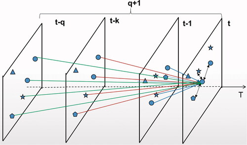
To make the methodology practical for most GIS users, this study incorporates temporal relations into the spatial weights matrix calculation as shown in Figure 2. The unidirectional temporal effect of SDPOT data means that future observations cannot influence past observations (Dubé and Legros 2012). This assumption is critical for spatiotemporal analysis with SDPOT, particularly when it covers a long duration. All observations are ordered chronologically so that the first right frame in the dataset corresponds to the newest observations, while the last left frame represents the oldest ones. In Figure 2, time t represents the actual time to be targeted; its temporal influence only subjected to neighbouring points at earlier times, that is, t-1,t-2,…t-q. q + 1 denotes the temporal duration, and q is the number of prior time periods. In this sense, at time t, q prior time periods (represented as separate layers) define the temporal bandwidth. But, at the time point t-k, only (q-k) prior time periods define the temporal bandwidth. At time t-q, there are no prior observations, so no temporal effects can be analyzed. This leads to the unbalanced temporal scale problem (UTSP), which will be further discussed at a later stage.

Figure 2. The scheme of the spatio-temporal matrix construction (t is the actual time point and q represents previous time points).

The spatial weight matrix was constructed in the following way. Only the spatial distance between points at actual time t and previous time t-k (k = 0, 1, …, q) is calculated by (Equation 10(12) $$S_{tk}={\left[\begin{array}{cccc}{s}_{1_t{1}_k}& s_{1_t{2}_k}& \dots & s_{1_t{N}_k}\\ s_{2_t{1}_k}& s_{2_t{2}_k}& \dots & s_{2_t{N}_k}\\ \dots & \dots & \dots & \dots \\ s_{N_t{1}_k}& s_{N_t{2}_k}& \dots & s_{N_t{N}_k}\end{array}\right]}_{N_t\times N_k},W_{\mathit{Spatial}}=\left[\begin{array}{c}{S}_{t0}\\ S_{t1}\\ \dots \\ S_{tq}\end{array}\right]$$(12) ). To concise the symbol, here we used the k denote the time (t-k). The spatial weight matrix at time k is denoted as $S_{\text{tk}}$ (Equation 12(12) $$S_{tk}={\left[\begin{array}{cccc}{s}_{1_t{1}_k}& s_{1_t{2}_k}& \dots & s_{1_t{N}_k}\\ s_{2_t{1}_k}& s_{2_t{2}_k}& \dots & s_{2_t{N}_k}\\ \dots & \dots & \dots & \dots \\ s_{N_t{1}_k}& s_{N_t{2}_k}& \dots & s_{N_t{N}_k}\end{array}\right]}_{N_t\times N_k},W_{\mathit{Spatial}}=\left[\begin{array}{c}{S}_{t0}\\ S_{t1}\\ \dots \\ S_{tq}\end{array}\right]$$(12) ): (12) $$S_{tk}={\left[\begin{array}{cccc}{s}_{1_t{1}_k}& s_{1_t{2}_k}& \dots & s_{1_t{N}_k}\\ s_{2_t{1}_k}& s_{2_t{2}_k}& \dots & s_{2_t{N}_k}\\ \dots & \dots & \dots & \dots \\ s_{N_t{1}_k}& s_{N_t{2}_k}& \dots & s_{N_t{N}_k}\end{array}\right]}_{N_t\times N_k},W_{\mathit{Spatial}}=\left[\begin{array}{c}{S}_{t0}\\ S_{t1}\\ \dots \\ S_{tq}\end{array}\right]$$(12) where ${\mathrm{N}}_{\mathrm{t}}$ and ${\mathrm{N}}_{\mathrm{k}}$ are the number of the points at time t and k, respectively. ${\mathrm{S}}_{\mathrm{t}0}$ means the spatial matrix at time t. It is worth noting that the spatial weights matrix ${\mathrm{S}}_{\mathrm{tk}}$ is not always a square matrix because the number of points at time t often differs from the number of points at time k. To reflect the whole spatial relation at time t, all the spatial weight matrices from previous time periods are summarized into a single matrix$\mathrm{ }{\mathrm{W}}_{\mathrm{Spatial}}$ which is a serrated matrix instead of a traditional matrix. Because this method just calculated the weight matrix between actual time t and all previous observations and not considered the interaction between previous observations, the total computation time is only 1/q of the computational time using the traditional method, so this method is particularly valuable for analysing a large SDPOT data set.

In the case of temporal relations, the same process is employed to construct the temporal weight matrix. Only the temporal distance between actual time t and previous time t-k (k = 0, 1, …, q) is calculated (Equation 11(11) $$T_{ij}=g(d_{ij}^t)=\{\begin{array}{c}{(d^t{}_{ij})}^{-\alpha }\begin{array}{c}\end{array}if\begin{array}{c}\end{array}and\begin{array}{c}\end{array}{d}^t{}_{ij}\le t_0\\ 0\begin{array}{ccc}\begin{array}{c}\end{array}& & \end{array}{d}^t{}_{ij}>t_0\end{array}$$(11) ). As ${\mathrm{T}}_{\mathrm{tk}}$ represents temporal relations between time t and observations collected at time k, pooling these individual values creates the global temporal weights matrix $W_{\mathit{Temporal}}$ in Equation 13(13) $$W_{\mathit{Temporal}}={\left[\begin{array}{cccccc}1& T_{t1}& \dots & T_{tk}& \dots & T_{tq}\end{array}\right]}^T$$(13) : (13) $$W_{\mathit{Temporal}}={\left[\begin{array}{cccccc}1& T_{t1}& \dots & T_{tk}& \dots & T_{tq}\end{array}\right]}^T$$(13) where the first element is 1, the time k and the target observations are in the same time period. The T at top right-hand corner is the sign of matrix transposition. The dimension of the temporal weight matrix is the same as the spatial matrix, but has a different meaning; it takes account of the unidirectional temporal relation between observations in all time periods.

Finally, the spatio-temporal weight matrix is constructed by multiplying the spatial weight matrix with the temporal weight matrix, term by term, as shown in Equation 14(14) $$W=W_{\mathit{Spatial}}•W_{\mathit{Temporal}}={\left[\begin{array}{c}{S}_{t0}\\ S_{t1}\\ \dots \\ S_{tq}\end{array}\right]}_{}•\left[\begin{array}{c}1\\ T_{t1}\\ \dots \\ T_{tq}\end{array}\right]$$(14) . Using this dot product scheme, Equation 14(14) $$W=W_{\mathit{Spatial}}•W_{\mathit{Temporal}}={\left[\begin{array}{c}{S}_{t0}\\ S_{t1}\\ \dots \\ S_{tq}\end{array}\right]}_{}•\left[\begin{array}{c}1\\ T_{t1}\\ \dots \\ T_{tq}\end{array}\right]$$(14) results in a number rather than a matrix. There are three other sophisticated schemes of integrating the spatial and temporal weight metrices, which result in a matrix: the Kronecker product (Shen et al. 2016, Liu et al. 2019), the Hadamard Product (Dubé and Legros 2015), and the matmul product (Huang et al. 2010, Fotheringham et al. 2015). (14) $$W=W_{\mathit{Spatial}}•W_{\mathit{Temporal}}={\left[\begin{array}{c}{S}_{t0}\\ S_{t1}\\ \dots \\ S_{tq}\end{array}\right]}_{}•\left[\begin{array}{c}1\\ T_{t1}\\ \dots \\ T_{tq}\end{array}\right]$$(14)

The dot product scheme used in this study has two obvious advantages of constructing the spatio-temporal weight over other schemes mentioned above. First, this method addresses the multidirectional spatial effect and the unidirectional temporal effect via two separate processes, which makes it easier to interpret the complex spatial-temporal patterns. Second, the simplified method is not only able to reduce computational time, but also makes it possible to update the weight matrix by focusing on spatial or temporal effects differently. For example, when the temporal weight is set as $W_{\mathit{Temporal}}={[1,\mathrm{ }1,\dots ,1]}^T,$ the temporal effect is least considered, and the spatial-temporal weight matrix is just equal to the spatial matrix; the geographically and temporally weighted colocation quotient turns into a geographically weighted colocation quotient. In the same way, when the spatial weight matrix is set as $W_{\mathit{Spatial}}={[1,\mathrm{ }1,\dots ,1]}^T,$ the geographically and temporally weighted colocation quotient becomes a temporally weighted colocation quotient. Mathematically, the dot or inner product scheme has been increasingly used in the computation of machine learning algorithms (Moura et al. 2020).

2.3. Monte Carlo simulation

To test the significance of spatio-temporal colocation quotient values, a Monte Carlo simulation method is used to calculate statistical test values. Monte Carlo simulation has been extensively used to estimate the variability of a chosen test statistic under the null hypothesis, in order to determine whether the test statistic calculated from the data deviates from the null hypothesis (Olden and Neff 2001, Myllymäki et al. 2021), such as in geographically weighted regression (Xu and Liang 2001, Brunsdon et al. 2010, Ren et al. 2014). In this study, the Monte Carlo simulation process select the category of each point randomly according the frequency distribution of each point category. A sampling distribution, in terms of the geographically and temporally weighted co-location quotient, is produced by repeating this process many times. Then, the sampling distribution are compared with the distribution of the observed values in order to derive a test statistic and its significance level. The pseudo-code of the Monte Carlo simulation is listed in Appendix A.

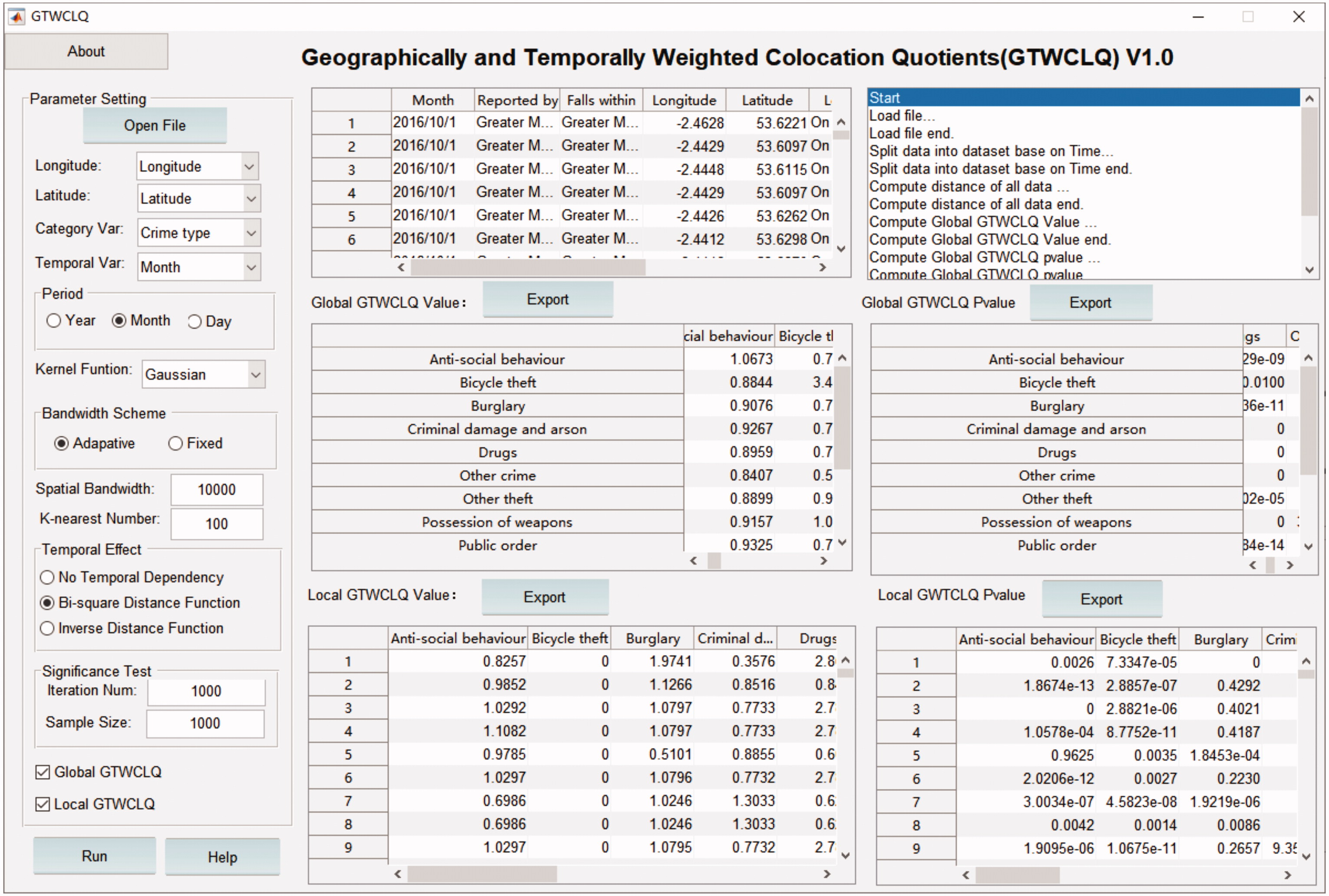
The sample size and the iteration times are the key parameters influencing the accuracy of significance test. A large sample size and a long iteration time will require lots of computational time while a smaller sample size and shorter iteration time will likely create an inaccurate result. Based on findings from previous studies (Zacharov et al. 2013, Hu et al. 2018), the sample size was set at 1000, and 1000 random simulations were run in this study. A P-value smaller than 0.05 indicates that the spatial-temporal colocation pattern is significant at the 95% confidence level (Wang et al. 2017). The interface of GTWCLQ software package developed by the team is shown in Appendix B.

3. Case study and results

3.1. Spatio-temporal crime data

Open source spatio-temporal recorded crime data for Greater Manchester in 2016 were used to validate the GTWCLQ method. Greater Manchester, a metropolitan authority in northwestern England, is comprised of 10 local authorities and has two cities (Manchester and Salford) as well as numerous towns and rural areas.

The UK police open data web service (data.police.uk) enables monthly point data of recorded crimes to be downloaded for any defined police authority. The data are categorised by crime type and include the longitude and latitude coordinates of each crime and the month in which it was recorded. This case study undertook crime pattern analysis using all 12 months of data from 2016. In this year, there were a total of 362,115 recorded crimes, across 14 categories of crime type, were recorded in Greater Manchester. The statistical and temporal distributions of the crimes are shown in Table 1 and Figure 3 respectively.

Figure 3. Temporal distribution of categorical crime data in 2016.

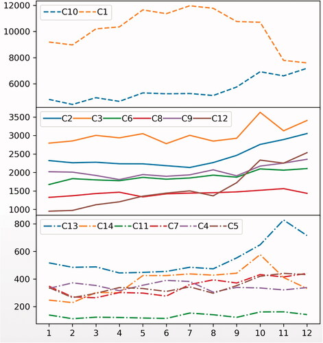
Table 1. Crime data categories and counts.

Code	Crime category	Count	Code	Crime category	Count
C1	Anti-social behavior	122319	C8	Shoplifting	17240
C2	Burglary	29086	C9	Vehicle crime	24298
C3	Criminal damage and arson	36363	C10	Violence and sexual offences	66175
C4	Drugs	4137	C11	Possession of weapons	1607
C5	Other crime	4163	C12	Public order	18776
C6	Other theft	22685	C13	Theft from the person	6540
C7	Robbery	4171	C14	Bicycle theft	4555

3.2. Geographically and temporally weighted CLQ (GTWCLQ) analysis of crime patterns

An adaptive bandwidth, rather than a fixed bandwidth, was selected for all the spatio-temporal crime analyses in this study given that Greater Manchester contains a mixture of urban and rural areas with consequent varying densities of socio-economic activities, recognizing that these tend to hold association with crime clustering (Yue et al. 2017, Wang et al. 2017). In several case studies, the relative optimal bandwidth is set around $\sqrt{\mathrm{N}}$ magnitude (N is the number of samples) (Hamada et al. 2015, Yuan et al. 2019). As an experimental test, the spatial bandwidth was set at $\sqrt{\mathrm{N}}$≈ 100. The sample size in the Monte Carlo simulation (significant test), therefore, was set to N = 1000, and the number of random iterations was set to M = 1000. The global GTWCLQ values, based on Equation 9(9) $$f(d_{ij}^s)\times g(d_{ij}^t)=w_{ij}{t}_k=W_{\mathit{ijk}}$$(9) and shown in Table 2, reflect the spatio-temporal association between crime categories in December 2016 (actual time), taking account of the temporal effects of prior months from January to November. As such, the temporal scale is 12 months and the spatial scale is 100, captured by the adaptive bandwidth value.

Table 2. The global geographically and temporally weighted GTWCLQ values for the 14 crime categories.

Type	C1	C2	C3	C4	C5	C6	C7	C8	C9	C10	C11	C12	C13	C14
C1	1.05	1.01	1.06	0.79	0.95	0.83	0.97	0.57	0.93	1.05		1.36	0.56	0.71
C2	0.69	2.62		0.84			1.02	0.39	1.19	1.04	0.69	1.14	0.43	0.79
C3	0.73	1.05	2.17	0.84	1.09	0.78	0.88	0.45	1.04		0.80	1.29	0.46
C4	0.71	1.10	1.04	7.96	1.42		0.92	0.55	0.88	1.15	1.69	1.25	1.00
C5	0.70	1.05		1.07	8.15	0.82	0.88	0.48	0.92	1.24	0.97	1.45	0.34	0.67
C6	0.70	1.05	0.97	0.81	0.98	2.37	1.10	0.77	0.94	1.09		1.23	1.20	1.08
C7	0.72	1.11	1.00		0.94	0.92	7.85	0.72	1.08	1.04	0.65		0.96	0.94
C8	0.62	0.64	0.66	0.58	0.56	0.99	1.14	6.59	0.54	0.73	1.12		1.14	1.01
C9	0.68	1.27			0.94	0.82	1.04	0.42	2.88	0.95		1.14	0.77	0.86
C10	0.73	1.04	1.03			0.89		0.50	0.88	1.65	0.79	1.34
C11	0.69	1.08		1.63		1.02	1.00		1.00		16.9	1.29	0.71	1.01
C12	0.76	0.93	1.02	0.82	1.11	0.85	1.07	0.66	0.88			3.08	0.55	0.77
C13	0.51	0.55	0.54	1.44	0.46	1.30	1.24	1.08	0.45	0.62		0.79	19.8	1.28
C14	0.68		0.86			1.10	1.08	0.95		0.94	1.04		1.24	8.17

Note: blank cells indicate insignificant values at 5% level.

All crime categories, taken individually, had a CLQ value of greater than 1 (bold, italic values in Table 2) along the diagonal line, although the CLQ values varied greatly between crime categories. In other words, all the crime categories were characterized by a degree of spatial autocorrelation when considering both spatial and temporal dependence or distance decay effects. C13 (theft from the person) showed the strongest clustering pattern, indicated by the largest CLQ value of 19.8.

The symmetrical and asymmetrical dependence between the 14 crime categories, identified and classified using the global GTWCLQ values in Table 2, are visualized in Figure 4. Among the symmetrically dependent pairs (Figure 4(a)), C4-C11 had the largest two-way GTWCLQ values (1.63 and 1.69), indicative of a strong co-location association between drug-related crimes (C4) and possession of weapon crimes (C11). Interestingly, two loops of co-location patterns between C2 (burglary), C7 (robbery) and C9 (vehicle crime), and between C6 (other theft), C13 (theft from the person) and C14 (bicycle theft) were also detected, suggestive of a small network community with strong spatio-temporal interactions between these categories, statistically. There might be a set of neighborhoods possessing facilities and/or land use features that serve to generate the strong spatio-temporal interactions between these categories.

Figure 4. The symmetrical (a) and asymmetrical dependence (b) between crime categories.

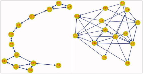
Figure 4(b) shows the many asymmetrical associations between crime categories. C12 (public order), C2 (burglary) and C7 (Robbery) were the most dependent categories, each having 7 other categories with GTWCLQ values in relation to them that were greater than 1 but not vice versa. This suggests that the social and/or physical characteristics of the locations of burglaries, robbery and public order offences serve to attract many other crimes. By contrast, C1 was the least spatially associated with other crimes, given that the GTWCLQ values from other categories to them were less than 1. This indicates that locations of anti-social behavior and shoplifting crimes were independent of other crime categories. C1 (anti-social behavior) was spatially excluded by others, which places it in an independent category. This is (potentially) explained by the fact that anti-social behavior crime tends to locate in residential neighborhoods and not city in center locations.

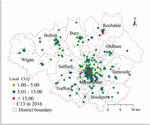
As with other GWSM methods, GTWCLQ is well suited for mapping local clusters of categories which have strong spatial and temporal dependence. A small selection of examples will be used to illustrate this point. C13 (theft from the person) had the largest global GTWCLQ value (19.8) of all crime categories (Table 2), such strong spatial autocorrelation is indicative of local clusters. Figure 5 shows the C13 data points that have local GTWCLQ^l values (Equation 6(6) $$\mathit{GTWCL}{Q}_{}^l(i)=\frac{\sum _{k\in E}\sum _{j\in D_k}^{}{W}_{\mathit{ijk}}{x}_{kj}}{M\sum _{k\in E}\sum _{j\in D_k}^{}{W}_{\mathit{ijk}}}$$(6) ) greater than 1 at a 5% significance level. The greater the local GTWCLQ^l value, the stronger the local spatial autocorrelation. Clusters were mostly located in Manchester city center (the largest concentration) and Rochdale town center (smaller concentration). This pattern can be explained by the higher densities of population attracted to the socio-economic activities in city/town centers than other areas.

Figure 5. Local clusters of GTWCLQ values for C13 (theft from the person).

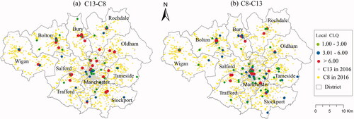
As shown in Figure 6(a), it is easy to understand the statistical artefact that shops attract people, who were required for the crime of shoplifting. In turn, shoppers are vulnerable to theft from a person. Consequently, the clusters of shops (i.e. city and town centers) are the destinations of shop lifting and theft from a person. As shown in Figure 6(b), there are factors other than shops that attract people to these locations.

Figure 6. Local clusters of symmetrical dependence (co-location association) between C13 (theft from a person) and C8 (shoplifting); (a) shows where C13 depends on C8, and (b) shows where C8 depends on C13.

Scaling effects in geographically weighted modelling have been widely discussed. The bandwidth value in GWSM indicates a kind of scale (Fotheringham et al. 2002), as it determines the number of neighboring points used for local calculations. In GTWCLQ, empirical tests, rather than a calibration process, are used to identify the optimal bandwidth value. GTWCLQ requires two bandwidth values that correspond to spatial and temporal scales. To test the impact of spatial and temporal scale effect, global GTWCLQ values were calculated for all 14 crime categories with itself in December 2016 using different spatial bandwidth and temporal bandwidth. The results listed in Tables 3 and 4.

Table 3. Global GTWCLQ values for 14 crime categories with itself based on four different spatial bandwidth values.

Type of crime	Adaptive bandwidth size
	K = 10	K = 100	K = 300	K = 500	Count
C1	1.78	1.05	0.88	0.86	122319
C2	6.81	2.62	1.76	1.62	29086
C3	4.90	2.17	1.46	1.38	36363
C4	33.28	7.96	3.00	2.55	4137
C5	31.54	8.15	4.24	5.00	4163
C6	7.24	2.37	1.60	1.51	22685
C7	30.11	7.85	3.42	2.90	4171
C8	9.39	6.59	5.13	4.57	17240
C9	7.32	2.88	1.85	1.73	24298
C10	2.99	1.65	1.37	1.34	66175
C11	86.55	16.91	14.77	12.67	1607
C12	7.56	3.08	2.00	1.88	18776
C13	14.99	19.82	9.97	8.54	6540
C14	31.13	8.17	3.74	3.12	4555

Note: Bandwidth K = 10, 100, 300 and 500 indicates that 10, 100, 300 and 500 nearest neighboring points were chosen for each target point; Count refers to the total number of points in that specific crime type. All colocation quotient values were significant at the 5% level.

Table 4. The Global GTWCLQ values for all 14 crime categories with itself and each of the four temporal bandwidth values.

Type of crime	Temporal bandwidth for crime type
	3_months	6_months	9_months	12_months
C1	1.07	1.00	1.01	1.05
C2	1.59	2.03	2.36	2.62
C3	1.42	1.76	1.99	2.17
C4	3.43	5.20	6.57	7.96
C5	3.87	5.44	6.51	8.16
C6	1.56	1.93	2.13	2.37
C7	3.03	4.46	6.21	7.85
C8	5.28	6.18	6.23	6.59
C9	1.78	2.24	2.63	2.88
C10	1.21	1.41	1.55	1.65
C11	15.25	10.82	14.33	16.91
C12	1.48	2.07	2.56	3.08
C13	8.47	13.49	16.85	19.82
C14	3.41	5.05	6.32	8.17

Note: temporal bandwidth T = 3, 6, 9 and 12 means that the closest three, six, nine and twelve month periods prior to December 2016 were used to select the neighbouring points for the GTWCLQ analyses (all values were significant at the 5% level.

Table 3 indicates that spatial autocorrelation was present in all crime categories except C1 (anti-social behavior), and for all spatial bandwidth values. C1 (anti-social behavior) had a dispersed, rather than clustered, pattern when the bandwidth was greater than 100. For all crime categories except C5 (other crime) and C13 (theft from the person), spatial autocorrelation decreased as the bandwidth size increased. C13 (theft from the person) had the highest level of spatial autocorrelation with a bandwidth value of 100, rather than 10 or 500. These results suggest crime patterns are spatially scale dependent as the large bandwidth value reduces the spatial autocorrelation.

Table 4 shows that all crime categories exhibited a clustering pattern (value >1) with each temporal bandwidth value. In general, spatial autocorrelation (clustering) increases as the temporal bandwidth increases, with the exception of the C1 and C11 crime categories. GTWCLQ values for C1 (anti-social behavior) were similar across all temporal bandwidth values (around 1), which suggests these types of crime are independent of temporal effects, or that there is no clear temporal effect. For C11 (possession of a weapon), the spatio-temporal pattern was least clustered at the 6-month temporal scale (10.82) and most clustered with a 1-year bandwidth value, suggestive of a strong temporal effect.

4. Discussion

The results presented above validate the application of GTWCLQ for spatio-temporal crime pattern analysis, and its suitability for mapping clusters and visualizing co-location patterns. The following sub-sections discuss three additional issues regarding the methodological and technical implementation of GTWCLQ.

4.1. Comparison between GTWCLQ and GWCLQ

The GTWCLQ presented in this paper was compared with GWCLQ. Using the same set of parameters (i.e., spatial bandwidth value of 100), three analyses including classical GWCLQ, where only one month of data was used (Wang et al. 2017), GTWCLQ1, where all time periods were given equal temporal weight, and GTWCLQ2, where temporal weights varied, were applied to C13 (theft from a person) crime data from December 2016. That is, the difference between no temporal effect, equal temporal effect, and heterogeneous temporal effect was evaluated. The results are shown in Table 5.

Table 5. The global values of GWCLQ, GTWCLQ1 and GTWCLQ2 for all crime categories in relation to C13.

Category	GWCLQ	GTWCLQ1	GTWCLQ2
C1	0.96	0.80	0.51
C2	0.47	0.46	0.55
C3	0.54	0.46	0.54
C4	0.96	1.43	1.44
C5	0.50	0.43	0.46
C6	1.71	1.67	1.30
C7	1.68	1.58	1.24
C8	2.25	2.66	1.08
C9	0.62	0.41	0.45
C10	0.69	0.76	0.62
C11	0.97
C12	0.91		0.79
C13	5.42	7.77	19.82
C14	1.83	1.91	1.28

Note: blank indicates an insignificant value.

First, the global CLQ value of C13 increased from 5.42 to 7.77 and then to 19.82 across the three methods (Table 5), which suggests that accounting for equal and heterogeneous temporal effects increases spatio-temporal autocorrelation. However, in some cases, adding temporal effects changed the dependence between some crime categories and the C13 (theft from the person) crime category. For example, the dependence of C6 (other theft) and C7 (robbery) on C13 (theft from the person) gradually decreased as increasingly complex temporal effects were included in the analysis. Two crime categories, C8 (shoplifting) and C14 (bicycle theft), were more dependent on C13 (theft from the person) when equal temporal effects were included, but had the lowest dependence when heterogeneous temporal effects were included. One category, C4 (drugs), only had a clustering pattern in relation to C13 when temporal effects were considered.

Figure 7 shows local values (>1) of C13 to C13 from each of the three CLQ methods. Fewer points and a more dispersed pattern were detected by GTWCLQ1 and GTWCLQ2 than GWCLQ, which suggests that including temporal effects helped to detect clusters in Rochdale and rural areas.

Figure 7. Spatial distribution of significant local values for C13 to C13 from (a) GWCLQ, (b) GTWCLQ1, (c) GTWCLQ2 and (d) the spatial distribution of merged clusters from three methods.

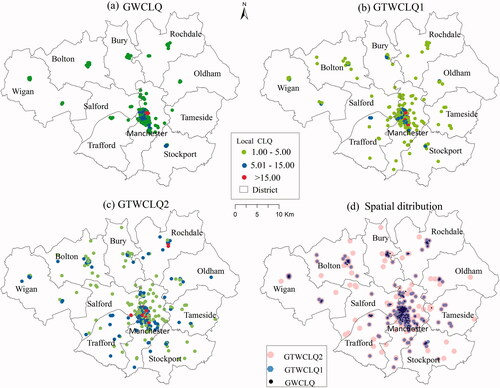
Further, covariance analysis, as listed in Table 6, is applied to compare the significant local values between three methods shown in Figure 7. It is clear to see there is significant disparity between the GWCLQ, GTWCLQ1, and GTWCLQ2 outputs at the 99% confidence level. This indicates the different statistical patterns when considering varying temporal effects. Selecting the same parameters of global Moran I: Gaussian kernel function and the spatial bandwidth of 100, the Moran I values of the three maps in Figure 7(a–c) are all greater than 0.95, which means three methods are all powerful in mapping local clusters. As shown in Figure 7(d), there are more local clusters from GTWCLQ2 when considering heterogeneous temporal effects.

Table 6. Comparisons in covariance analysis between the three methods (at 1% significance level).

Method I	Method J	I-means	J-means	I-J	p-value
GTWCLQ2	GWCLQ	10.77	8.38	2.39	0.000**
GTWCLQ2	GTWCLQ1	10.77	5.88	−4.88	0.000**
GTWCLQ1	GWCLQ	8.38	5.88	2.49	0.000**

4.2. Unbalanced temporal scale problem

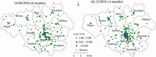
Due to the unbalanced temporal scale problem (UTSP) with SDPOT data, discussed earlier, a temporal scale or duration of 12 months is only possible when analyzing crime patterns in December 2016. The largest temporal scale for crime pattern in June 2016 can only include data for 6 months (January to June) due to the unidirectional temporal effect detailed in Section 2 of this paper. In order to compare the spatio-temporal patterns between June and December, a same temporal scale (number of time periods) must be selected, in this case, which is 6 months at maximum. This means the 6-month data from January to June used for June pattern and another 6-month data from July to December used for December patterns. By selecting 100 as spatial bandwidth and 6 as temporal bandwidth, the local GTWCLQ was run for spatio-temporal pattern analysis in June and December respectively. Clusters from the June and December patterns (only significant local values greater than 1) are shown in Figure 8(a-June pattern and b-December pattern). Figure 8 shows the distribution of significant GTWCLQ values and local clusters of C13 (theft from the person) in both June and December 2016. Comparison of the two patterns in Figure 8 shows that C13 (theft from the person) had a more clustered pattern in June than in December. This might be explained by the existence of a greater number of shopping activities/locations in the Christmas period (December). Consequently, the unbalanced temporal scale problem can be indirectly explored by reducing temporal scales (number of time periods) when comparing the spatio-temporal patterns at two time periods. For example, when choosing 2-month as temporal scale, the patterns from February to December can be compared. However, this method is not the best solution in practice due to data limitation since a fixed temporal scale (e.g. half a year) might be needed for comparisons between all time periods.

Figure 8. Spatial distributions of significant (at 5% level) local values of GTWCLQ for C13: (a) The values of June in 2016 using 6 months, (b)The values of December in 2016 using 6 months.

4.3. Computational complexity

In addition to scale issues, achieving computational efficiency is a challenge for GTWCLQ because the distance matrix and significance test calculations are time and memory intensive, as they are in other GWM approaches (Harris et al. 2010, Zhang et al. 2017). Using the following hardware and software (PC computer: CPU: Intel i9-9900K, 3.6 GHz, 16 Core, RAM: 32.0 GB, Matlab 2015 b), the computational times for running GTWCLQ with different temporal scales (3, 6, 9 and 12 months) and a single spatial scale (adaptive bandwidth of 100) are listed in Table 7.

Table 7. Runtime (in seconds) of GTWCLQ with 4 temporal bandwidths (3 m–12m).

Bandwidth	Number	Global GTWCLQ				Local GTWCLQ
		Matrix	Global	MC	Total	Matrix	Local CLQ	MC	Total
3_m	97910	327	1.59	116	444.59	352	1.53	129	482.53
6_m	221190	655	2.61	207	864.61	712	2.91	222	936.91
9_m	280170	902	3.28	309	1214.3	1064	2.98	313	1380
12 m	362115	1189	4.15	397	1590.2	1378	3.94	423	1804.9

Note: the runtime for the matrix includes calculation and sorting of the distance matrix. MC is the runtime of significant tests using a Monte Carlo simulation (N = 1000, M = 1000). Total refers to the runtime for all processes.

The results clearly demonstrate (as expected) that the runtime for local GTWCLQ is longer than that for global GTWCLQ, and the calculation of the matrix takes much longer than GTWCLQ computation and the Monte Carlo test. Deploying longer or more fine-grained temporal scales will inevitably increase the number of points used in analyses and will increase the total runtime. The complexity of the algorithm also requires significant storage space. For a case study of 100,000 data points (n = 100,000), 38GB of memory would be needed to save an n × n distance matrix when a 32-bit float type is used to denote calculated values.

5. Conclusions

Categorical SDPOT data, characterized by point features with high spatial and temporal resolutions but unidirectional time effects, require unique spatio-temporal analysis methods. The co-location quotient and the more recently developed geographically weighted co-location quotient (GWCLQ) have been used successfully to analyze the spatial dependence and heterogeneity of this type of data. This paper has presented a further innovation – the geographically and temporally weighted co-location quotient (GTWCLQ) – which considers spatio-temporal dependence and heterogeneity in categorical SDPOT data. This new approach includes global and local computations of GTWCLQ and proposes a significance test using a Monte Carlo simulation. The integration of spatial and temporal weight matrices is based on a dot product, and this method can reduce computational time as well as make it easy to transfer to only geographically or temporally weighted co-location quotient analysis. The key decision in implementing adaptive GTWCLQ is the selection of spatial and temporal bandwidth values, which dictate the number of neighboring points and the time periods to be used in the analysis.

This approach has been efficiently validated in a case study of spatio-temporal crime patterns across Greater Manchester in 2016. The categorical SDPOT crime data included 14 categories or types of recorded crime. Using the GTWCLQ approach, the spatio-temporal association between 14 crime categories was analyzed for December 2016, taking account of spatio-temporal effects from prior months and neighboring places. The key results from the GTWCLQ analysis, with a spatial bandwidth of 100 points and a temporal bandwidth of 12 months, can be described as follows. Firstly, all the crime categories, as expected given the existing criminological literature (Weisburd 2015), exhibited varying degrees of spatial clustering. That said, ‘theft from a person’ held the strongest spatio-temporal dependence and produced the largest clusters, located in Manchester city centre and Rochdale town center. Secondly, there were 15 pairs of crime categories with co-location patterns, among which drug (C4) and possession of a weapon (C11) crimes held the largest co-location association. Interestingly, two loops of co-location patterns between C2 (burglary), C7 (robbery) and C9 (vehicle crime), and between C6 (other theft), C13 (theft from the person) and C14 (bicycle theft) were detected, suggestive of a small network community with strong spatio-temporal interactions between these categories. Thirdly, there were many asymmetrical associations between categories, although C1 (anti-social behavior) was spatially excluded by others, suggesting this forms an independent category. Evidence of the spatial and temporal colocation and symmetry of crimes might usefully be deployed to inform the development of criminological theory, serving to help disentangle the relationships between crime and the urban environment, recognizing that crimes are associated with a combination of facilities and land use features that draw populations (offenders and victims) to these locations (Bannister and OSullivan 2021).

It should be noted that the results refer to crime spatio-temporal patterns in December 2016. To compare patterns from different time periods (e.g., June and December), the same spatial and temporal scales (duration) must be used, such as 6 months. This paper tends to highlight this unbalanced temporal scale problem (UTSP) in spatio-temporal pattern analysis with SDPOT data, which is different from the modifiable temporal unit problem (Cheng and Adepeju 2014). The former is influenced by the varying temporal scale at time period but the latter by the temporal aggregation of data.

Based on our experimental tests, the spatial scale (bandwidth size) at which maximum spatial autocorrelation occurred varied between crime categories. By contrast, spatial autocorrelation increased as temporal scale (duration) increased across all categories. These tests highlight the importance of choosing appropriate spatial and temporal scales in GTWCLQ analysis.

This paper also has some limitations. The impact of different (spatial and time) distance decay effects on crime patterns have not been examined although there are already many studies in the literature. The computational complexity of GTWCLQ could be reduced in future by using GPU based parallel computation (Wang et al. 2020b). Using hourly data or temporal scale by seasons might help detect more interesting spatio-temporal crimes patterns and this should be explored with high-quality data in the future. In line with the existing criminological evidence base, it would be valuable to consider the seasonal, weekly and daily distribution of crime counts, by crime count.

Acknowledgements

The authors thank the two anonymous reviewers and the editor for their constructive comments, which have helped improve this research paper.

Disclosure statement

No potential conflict of interest was reported by the author(s).

Data and code availability statement

The data and code for the method that supports the findings of this study are available with the identifier at the following link https://doi.org/10.6084/m9.figshare.16641763

Additional information

Funding

The National Natural Science Foundation of China [grant no. 41961062 and no. 42071135], the Guangxi Special Project of Science and Technology Base and Talents [grant no. AD19110142].

Notes on contributors

Ling Li

Ling Li is an associate professor in GIS. Her expertise includes geospatial modelling by fusing AI and mathematical modelling into big data analytics. Li’s recent projects focus on analysing and modeling spatial-temporal data to support predictive policy making.

Jianquan Cheng

Jianquan Cheng is a Reader in Urban Studies and deputy director of the Manchester Metropolitan Crime and Wellbeing Big Data Center. Research experiences and expertise include urban growth, geographical mobility, spatial accessibility, and sustainable healthy city, using GIS and big data approaches. His recent projects focus on analysing and modelling how physical and built-environment impacts on public health and well-being at a variety of scales in Chinese and British cities, which aim to generate data driven evidence and frameworks for spatial planning and governance.

Jon Bannister

Jon Bannister FAcSS FRSA (Fellow of the Academy of Social Sciences & Fellow of the Royal Society of Arts) is Professor of Criminology, who directs the Manchester Metropolitan Crime and Well-Being Big Data Centre. He holds research expertise in criminology, urban studies, sociology, social policy, big data, policing, evidence-based policy, advanced quantitative methods and knowledge mobilisation (inclusive of co-production). His research examines the interplay of urban processes and behaviours (urban transformations) upon the exposure to crime and other harms.

Xiongfa Mai

Xiongfa Mai is an associate professor in machine learning, whose expertise is deep learning and precipitation forecasting including intelligent optimisation algorithms. His research projects mainly focus on spatio-temporal series prediction using the deep learning approach.

JC: conceptual and methodological design, writing and revision, and supervision; LL: methodological design, technical implementation, writing and revision; JB: validation of the approach, interpretation of the results, and revision; MX: technical implementation, software development, and revision.

Appendix A.

The pseudo-code of the Monte Carlo simulation

Algorithm:

the significance test of global $\mathrm{GTWCLQ}$

Input: Dataset D which contains q + 1 sub datasets, each corresponding to a time.

Input: the global GTWCLQ from the dataset D

input: spatial bandwidth(b0), temporal bandwidth (t0), Kernel function (kf), test time (N), sample size (M)

Output: p-value

1. Iterations

For i = 1 to N

1. Generate the ${\mathrm{j}}^{\mathrm{th}}$ simulated samples${\text{ E}}_{\mathrm{j}}$ randomly from the dataset D by the method of stratified sampling, where the sample${\text{ E}}_{\mathrm{j}}$ contains q sub datasets, each corresponding to a time and the sample size of each sub dataset is M.

2. Calculate the GTWCLQ of the jth random sample E_j using Equation (8)(8) $$d^t{}_{ij}=t_i-t_j+1$$(8) with parameters b0, t0, kf, and store the result as mcGTWCLQ(j).

End

2. Calculate the average value avg_mcGTWCLQ of all mcGTWCLQ: $$\mathit{mcGTWCLQ}\mathrm{ }\leftarrow \mathrm{ }\frac{\sum _1^N\mathit{mcGTWCLQ}\left(j\right)}{N}$$

3. Calculate the standard deviation std_mcGTWCLQ of all mcGTWCLQ: $$\mathit{std}\_\mathit{mcGTWCLQ}\mathrm{ }\leftarrow \mathrm{ }\frac{\sqrt{\sum _1^N{\mathit{mcGTWCLQ}\left(j\right)-\mathit{avg}\_\mathit{mcGTWCLQ})}^2}}{N-1}$$

4. Taking GTWCLQ as the mean and std_mcGTWCLQ as the standard deviation, a normal distribution data points T relative to avg_mcGTWCLQ are constructed: $$\mathrm{T}=\left|\frac{\mathit{avg}\_\mathit{mcGTWCLQ}-\mathit{GTWCLQ}}{\mathit{std}\_\mathit{mcGTWCLQ}/\sqrt{N}}\right|\sim t\left(N\right);$$

5. Calculate the value of the bilateral cumulative distribution function of T, that is, get the value of P: $$\text{P value}\leftarrow 2\mathrm{*}(1-\mathrm{cdf}(\text{ 'norm'},\mathrm{ }\mathrm{T}\left)\right);\mathrm{ }\left(\text{ cdf is the cumulative distribution function}\right).$$

6. Output the p-value

End

(Note: the significance test of local GTWCLQ values follows the same process)

Appendix B.

The interface of GTWCLQ package developed by the project team

References

- Anderson, T.K., 2009. Kernel density estimation and K-means clustering to profile road accident hotspots. Accident; Analysis and Prevention, 41 (3), 359–364.
- Ansari, M.Y., et al., 2019. Spatiotemporal clustering: a review. Artificial Intelligence Review, 53 (4), 2381–2423.
- Atluri, G., Karpatne, A., and Kumar, V., 2019. Spatio-temporal data mining. ACM Computing Surveys, 51 (4), 1–41.
- Bannister, J., and O'Sullivan, A., 2021. Big data in the city. Urban Studies, 58 (15), 3061–3070.
- Batty and Michael 2016. Big data and the city. Built Environment, 42 (3), 321–337.
- Brunsdon, C., 1995. Estimating probability surfaces for geographical point data: An adaptive kernel algorithm. Computers & Geosciences, 21 (7), 877–894.
- Brunsdon, C., Fotheringham, A.S., and Charlton, M.E., 2010. Geographically weighted regression: a method for exploring spatial nonstationarity. Geographical Analysis, 28 (4), 281–298.
- Cao, W., et al., 2017. Location patterns of urban industry in Shanghai and implications for sustainability. Journal of Geographical Sciences, 27 (7), 857–878.
- Cheng, T., and Adepeju, M., 2014. Modifiable temporal unit problem (MTUP) and its effect on space-time cluster detection. PLoS One, 9 (6), e100465.
- Cho, S.-H., Lambert, D.M., and Chen, Z., 2010. Geographically weighted regression bandwidth selection and spatial autocorrelation: an empirical example using Chinese agriculture data. Applied Economics Letters, 17 (8), 767–772.
- Cleveland, W.S., 1979. Robust locally weighted regression and smoothing scatterplots. Journal of the American Statistical Association, 74 (368), 829–836.
- Corcoran, J., et al., 2021. The temporality of place: Constructing a temporal typology of crime in commercial precincts. Environment and Planning B: Urban Analytics and City Science, 48 (1), 9–24.
- Cromley, R.G., Hanink, D.M., and Bentley, G.C., 2014. Geographically weighted colocation quotients: specification and application. The Professional Geographer, 66 (1), 138–148.
- Dubé, J., and Legros, D., 2012. A spatio-temporal measure of spatial dependence: An example using real estate data. Papers in Regional Science, 92, 19–30.
- Dubé, J., and Legros, D., 2013. Dealing with spatial data pooled over time in statistical models. Letters in Spatial and Resource Sciences, 6 (1), 1–18.
- Dubé, J., and Legros, D., 2015. Modeling spatial data pooled over time: schematic representation and monte carlo evidences. Theoretical Economics Letters, 05 (01), 132–154.
- Dubé, J., Legros, D., and Thanos, S., 2018. Past price ‘memory’ in the housing market: testing the performance of different spatio-temporal specifications. Spatial Economic Analysis, 13 (1), 118–138.
- Dubin, R., Pace, R.K., and Thibodeau, T.G., 1999. Spatial autoregression techniques for real estate data. Journal of Real Estate Literature, 7 (1), 79–96.
- Eckardt, M., and Mateu, J., 2021. Partial and semi‐partial statistics of spatial associations for multivariate areal data. Geographical Analysis, 53 (4), 818–835.
- Emani, C.K., Cullot, N., and Nicolle, C., 2015. Understandable big data: a survey. Computer Science Review, 17 (AUG), 70–81.
- Ferreira, L.N., et al., 2020. Spatiotemporal data analysis with chronological networks. Nature Communications, 11 (1), 4036.
- Fotheringham, A.S., Brunsdon, C.F., and Charlton, M.E., 2002. Geographically Weighted Regression: The Analysis of Spatially Varying Relationships.
- Fotheringham, A.S., Crespo, R., and Yao, J., 2015. Geographical and temporal weighted regression (GTWR). Geographical Analysis, 47 (4), 431–452.
- Fotheringham, A.S., and Oshan, T.M., 2016. Geographically weighted regression and multicollinearity: dispelling the myth. Journal of Geographical Systems, 18 (4), 303–329.
- Hamada, N., et al., 2015., Population Synthesis via k-Nearest Neighbor Crossover Kernel. ed. 2015 IEEE International Conference on Data Mining (ICDM),
- Harris, P., et al., 2015. Enhancements to a geographically weighted principal component analysis in the context of an application to an environmental data set. Geographical Analysis, 47 (2), 146–172.
- Harris, R., et al., 2010. Grid-enabling geographically weighted regression: a case study of participation in higher education in England. Transactions in GIS, 14 (1), 43–61.
- Helbich, M., and Leitner, M., 2017. Frontiers in spatial and spatiotemporal crime analytics—an editorial. ISPRS International Journal of Geo-Information, 6 (3), 73.
- Hu, Y., Zhang, Y., and Shelton, K.S., 2018. Where are the dangerous intersections for pedestrians and cyclists: A colocation-based approach. Transportation Research Part C: Emerging Technologies, 95, 431–441.
- Huang, B., Wu, B., and Barry, M., 2010. Geographically and temporally weighted regression for modeling spatio-temporal variation in house prices. International Journal of Geographical Information Science, 24 (3), 383–401.
- Jefferson, B.J., 2018. Predictable policing: predictive crime mapping and geographies of policing and race. Annals of the American Association of Geographers, 108 (1), 1–16.
- Kandt, J., and Batty, M., 2021. Smart cities, big data and urban policy: towards urban analytics for the long run. Cities, 109, 102992.
- Kharrazi, A., Qin, H., and Zhang, Y., 2016. Urban big data and sustainable development goals: challenges and opportunities. Sustainability, 8 (12), 1293.
- Lee, J., and Li, S., 2017. Extending Moran's Index for measuring spatiotemporal clustering of geographic events. Geographical Analysis, 49 (1), 36–57.
- Li, Z., Cheng, J., and Wu, Q., 2016. Analyzing regional economic development patterns in a fast developing province of China through geographically weighted principal component analysis. Letters in Spatial and Resource Sciences, 9 (3), 1–13.
- Liu, J., et al., 2019. Pedestrian injury severity in motor vehicle crashes: an integrated spatio-temporal modeling approach. Accident; Analysis and Prevention, 132, 105272
- Liu, J., et al., 2020. Urban big data fusion based on deep learning: An overview. Information Fusion, 53, 123–133.
- Moura, J., et al., 2020. On the design and analysis of structured-ANN for online PID-tuning to bulk resumption process in ore mining system. Neurocomputing, 402, 266–282.
- Myllymäki, M., Kuronen, M., and Mrkvička, T., 2021. Testing global and local dependence of point patterns on covariates in parametric models. Spatial Statistics, 42, 100436.
- Nakaya, T., et al., 2005. Geographically weighted Poisson regression for disease association mapping. Statistics in Medicine, 24 (17), 2695–2717.
- Olden, J., and Neff, B., 2001. Cross-correlation bias in lag analysis of aquatic time series. Marine Biology, 138 (5), 1063–1070.
- Piza, E.L., and Carter, J.G., 2018. Predicting initiator and near repeat events in spatiotemporal crime patterns: an analysis of residential burglary and motor vehicle theft. Justice Quarterly, 35 (5), 842–829.
- Pope, M., and Song, W., 2015. Spatial relationship and colocation of crimes in Jefferson County, Kentucky. Papers in Applied Geography, 1 (3), 243–248.
- Quick, M., Law, J., and Li, G., 2019. Time-varying relationships between land use and crime: A spatio-temporal analysis of small-area seasonal property crime trends. Environment and Planning B: Urban Analytics and City Science, 46 (6), 1018–1035.
- Ren, T., et al., 2014. Moran's I test of spatial panel data model — Based on bootstrap method. Economic Modelling, 41, 9–14.
- Shen, C., Li, C., and Si, Y., 2016. Spatio-temporal autocorrelation measures for nonstationary series: A new temporally detrended spatio-temporal Moran's index. Physics Letters A, 380 (1-2), 106–116.
- Spettl, A., et al., 2015. Stochastic 3D modeling of Ostwald ripening at ultra-high volume fractions of the coarsening phase. Modelling and Simulation in Materials Science and Engineering, 23 (6), 065001.
- Tobler, W.R., 1970. A computer movie simulating urban growth in the detroit region. Economic Geography, 46, 234–240.
- Vega-Oliveros, D.A., et al., 2019. From spatio-temporal data to chronological networks. 675–682.
- Wang, D., et al., 2020b. A CUDA-based parallel geographically weighted regression for large-scale geographic data. ISPRS International Journal of Geo-Information, 9 (11), 653. doi:.
- Wang, D., Miwa, T., and Morikawa, T., 2020a. Big trajectory data mining: a survey of methods, applications, and services. Sensors, 20 (16), 4571.
- Wang, F., et al., 2017. Local indicator of colocation quotient with a statistical significance test: examining spatial association of crime and facilities. The Professional Geographer, 69 (1), 22–31.
- Wang, Z., and Lam, N.S.N., 2020. Extending getis–ord statistics to account for local space–time autocorrelation in spatial panel data. The Professional Geographer, 72 (3), 411–420.
- Weisburd, D., 2015. The law of crime concentration and the criminology of place. Criminology, 53 (2), 133–157.
- Wu, C., et al. 2018. Multiscale geographically and temporally weighted regression: exploring the spatiotemporal determinants of housing prices. International Journal of Geographical Information Science, 33 (3), 489-511.
- Xu, Q.-S., and Liang, Y. Z., 2001. Monte Carlo cross validation. Chemometrics and Intelligent Laboratory Systems, 56 (1), 1–11.
- Yang, B., et al., 2020. A spatio-temporal method for crime prediction using historical crime data and transitional zones identified from nightlight imagery. International Journal of Geographical Information Science, 34 (9), 1740–1725.
- Yousfi, S., et al., 2020. Mass appraisal without statistical estimation: a simplified comparable sales approach based on a spatiotemporal matrix. The Annals of Regional Science, 64 (2), 349–365.
- Yuan, K., et al., 2019. A quad-tree-based fast and adaptive Kernel Density Estimation algorithm for heat-map generation. International Journal of Geographical Information Science, 33 (12), 2455–2476.
- Yue, H., et al., 2017. The local colocation patterns of crime and land-use features in Wuhan. ISPRS International Journal of Geo-Information, 6 (10), 307.
- Zacharov, P., Rezacova, D., and Brozkova, R., 2013. Evaluation of the QPF of convective flash flood rainfalls over the Czech territory in 2009. Atmospheric Research, 131, 95–107.
- Zahnow, R., and Corcoran, J., 2021. Crime and bus stops: An examination using transit smart card and crime data. Environment and Planning B Urban Analytics and City Science, 48 (4), 706–723.
- Zhang, G., Zhu, A.X., and Huang, Q., 2017. A GPU-accelerated adaptive kernel density estimation approach for efficient point pattern analysis on spatial big data. International Journal of Geographical Information Science, 31 (10), 2068–2097.
- Zhang, L., Cheng, J., and Jin, C., 2019. Spatial interaction modeling of OD flow data: comparing geographically weighted negative binomial regression (GWNBR) and OLS (GWOLSR). ISPRS International Journal of Geo-Information, 8 (5), 220.