Multi-nomenclature, multi-resolution joint translation: an application to land-cover mapping

Abstract

Land-use/land-cover (LULC) maps describe the Earth’s surface with discrete classes at a specific spatial resolution. The chosen classes and resolution highly depend on peculiar uses, making it mandatory to develop methods to adapt these characteristics for a large range of applications. Recently, a convolutional neural network (CNN)-based method was introduced to take into account both spatial and geographical context to translate a LULC map into another one. However, this model only works for two maps: one source and one target. Inspired by natural language translation using multiple-language models, this article explores how to translate one LULC map into several targets with distinct nomenclatures and spatial resolutions. We first propose a new data set based on six open access LULC maps to train our CNN-based encoder-decoder framework. We then apply such a framework to convert each of these six maps into each of the others using our Multi-Landcover Translation network (MLCT-Net). Extensive experiments are conducted at a country scale (namely France). The results reveal that our MLCT-Net outperforms its semantic counterparts and gives on par results with mono-LULC models when evaluated on areas similar to those used for training. Furthermore, it outperforms the mono-LULC models when applied to totally new landscapes.

Keywords:

• Land-cover
• land-use
• translation
• deep learning
• harmonization

1. Introduction

Through considerable improvement in remote sensing techniques over the last three decades, a large number of land-use/land-cover (LULC) maps are now available (Grekousis et al. 2015, Mallet and Le Bris 2020) at multiple scales. This paves the way for more automatic, richer and finer representations of the ‘(bio)physical cover on the Earth’s surface’ (Gregorio 2000). LULC translation (Yang et al. 2017) aims to transform the inner characteristics of a given map to another one (either or both spatial resolution and classes). Due to the high complexity in generating new maps (computing and memory usage, reproducibility), translation appears an utmost important task for many operational applications, such as LULC fusion, harmonization, comparison and update (Pérez-Hoyos et al. 2020, Fritz and See 2005, Baudoux et al. 2021, Brown and Duh 2004). However, the challenge in map-to-map translation lies in the difficult interleaved association of semantic and spatial resolutions of both maps.

Usually, two different LULC establish complex relationships between their classes (Jansen et al. 2008) and straightforward one-to-one association is most of the time infeasible. Some classes may encompass highly distinct concepts and characteristics depending on the map, leading either to strong semantic overlap or inconsistencies. For example, the two generic land-cover classes forest areas and shrubs have varying definitions, depending on how tree height, density or minimal surface information have been taken into account (Comber et al. 2005). In parallel, we often note discrepant spatial resolutions depending on the data and the procedure used for map creation. While the spatial gap can be easily solved through ad-hoc image up- or down-sampling, this solution ignores the spatial information embedded into class definitions (Xu et al. 2014).

Such complexity may explain the limited literature in the field and why both dimensions are separately handled. The most common method for solving LULC translation consists today in a nomenclature-level semantic association followed by a separate spatial resampling strategy (Waser and Schwarz 2006, Schepaschenko et al. 2015, Lu et al. 2017, Ma et al. 2020).

Semantic association can be assessed in several ways, the most common technique being the comparison of a list of discrete characteristics of each LULC class (Ahlqvist 2008). The most well-known approach is probably the land cover classification system (LCCS) framework (Di Gregorio 2005), which computes the ratio of shared attributes between two classes to assess their semantic similarity. However, such family of approaches fail to translate complex relationships, often acting as a word-by-word translation. Spatial context is disregarded and, despite acknowledging multiple possible associations, each class is exclusively assigned to its strongest correspondent in the other nomenclature. Moreover, by processing the nomenclature translation separately from the change of spatial resolution, such approaches neglect semantic considerations on pixels holding multiple classes.

One recently proposed solution (Baudoux et al. 2021) introduced a convolutional neural network (CNN) based encoding-decoding strategy to foster context information extraction in an object-level LULC map translation, and achieved promising results. The core idea lied in the possibility for each map pixel of being translated differently, depending on its close surrounding pixels and its geographical context. However, this supervised method was designed as a mono-LULC translation. It required the two maps to at least partially spatially overlap. When impossible, a pivotal map that spatially overlaps the two others might be used but this would drastically lessen the translation performance by requiring two translations instead of a single one. Moreover, deriving this framework for multiple LULC translations requires multiple separate training phases and could perform poorly on land-cover maps with few training samples.

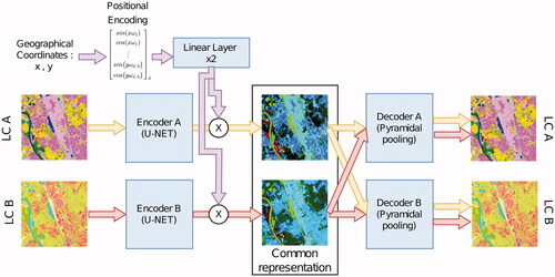
Recently, deep learning methods have achieved state-of-the-art results in natural language processing and, more precisely, in language translation (Conneau et al. 2020, Tran et al. 2021). Current state-of-the-art methods have shown the superiority of multi-lingual trained models against their mono-lingual counterparts (Conneau et al. 2020), especially on languages with a small number of translation examples. Multi-language training seems to benefit from the obtained multi-language common representation space (Pires et al. 2019). Finding shared representations is also frequently addressed by the remote sensing community for combining multi-modal data from various sensors, with varying resolutions and information into a compact and discriminative embedding (Mura et al. 2015, Audebert et al. 2018, Hong et al. 2021a, 2021b). Surprisingly, exception made of the previously mentioned semantic-based nomenclature harmonization framework (Baudoux et al. 2021), this question remains unaddressed for the LULC translation task at an object level. In this article, we tackle these issues by answering the following question: can we find a shared space for multi-LULC translation that would be beneficial for their individual generation? We propose a CNN -based solution that learns to simultaneously translate the spatial resolution and the nomenclature context with a common representation space (Figure 1). Our approach also exhibits a self-reconstruction ability which is highly beneficial to ensure that no information is lost during the mapping to the shared space.

Figure 1. Overall multi-LULC translation architecture. Our network (blue boxes) is trained to perform both self-reconstruction and translation. There is no restriction in the number of maps that can be embedded into our shared representation. For convenience, we only represent two maps (A and B). Red and orange arrows represent the possible paths for maps A and B. Note that at inference, only one of the two maps is required.

The main contributions of this paper are summarised as follows:

• We propose the first multi-LULC translation model that both handles the spatial and semantic dimensions of maps.

• A France-wide data-set including 6 open access LULC maps and a 2,300 point reference set available at https://doi.org/10.5281/zenodo.5843595.

• We conduct a comparative evaluation of the approach with semantic baselines and the supervised mono-LULC translation of Baudoux et al. (2021), supported by a carefully designed ground truth.

The proposed model, named Multiple Land-Cover Translation Network (MLCT-Net), achieves a significant performance enhancement compared to semantic methods and similar results with the mono-LULC context-based translation demonstrating the interest of training one unique multi-translation model over multiple independent ones. Moreover, MLCT-Net outperforms its mono-LULC counterparts when generalising to landscape types unseen during training. The remainder of this articlei s organised as follows. In Section 2, we briefly review some related works on LULC harmonisation and common space representation methods. Section 3 presents our data-set. Section 4 presents our architecture and training procedure. Experiments and results are presented in Section 5. Finally, we conclude this article with some remarks. The full implementation is made available at https://doi.org/10.5281/zenodo.7019838.

2. Related work

In this section, we first review the proposed approaches for LULC translation, underlining their main limitations. We then describe recent works on shared representation spaces showing their potential for LULC translation.

2.1. LULC translation

Finding a shared representation method applicable to all LULC is an old goal in the remote sensing community. Yang et al. (2017) separate two approaches: (1) standardisation which aims to natively produce maps with identical characteristics through the use of a universal nomenclature, and (2) harmonisation which aims to define methods for adapting the nomenclature of already existing maps with different characteristics.

2.1.1. Nomenclature standardisation

Standardisation approaches have been a main subject of concern since the early days of remote sensing, starting in the 1970s with the Anderson’s classification system (Anderson et al. 1976), followed by the well-known LCCS (Di Gregorio 2005), and more recently the EAGLE framework (Arnold et al. 2015). These frameworks propose toolboxes to build universal nomenclatures based on a grid of semantic attributes which are combined to obtain specific classes. These attributes are usually defined to be scale-independent, making these nomenclatures robust to spatial resolution changes. However, they do not guarantee obtaining the desired set of classes (Jansen et al. 2008). These methods are by nature designed to be applied before the conception of the LULC map, but are sometimes also proposed for harmonising existing maps.

2.1.2. Nomenclature harmonisation

Current LULC harmonisation methods are primarily focused on proposing a semantic mapping scheme between source and target classes. The spatial resolution change is carried out either before (Pérez-Hoyos et al. 2017) or after nomenclature translation (Raposo et al. 2017), without considering an interleaved procedure. Harmonisation methods can be categorised according to the semantic translation strategy. The most common strategy consists in manually matching the two nomenclatures through human visual inspection (Adamo et al. 2014). This strategy has the advantage of simplicity albeit not allowing a refined understanding of the quality of this match. This also prevents reproducibility and transfer to other LULC matching challenges. Therefore, numerous solutions have been proposed to automatically estimate the similarity between classes (Comber et al. 2004, Jepsen and Levin 2013). Similarity can, among other things, be computed on semi-lattices (Kavouras and Kokla 2002) or hierarchical tree representations of the nomenclature (Al-Mubaid and Nguyen 2009) or, more commonly, by comparing the semantic content of each class (Rodríguez et al. 1999, Feng and Flewelling 2004, Ahlqvist 2005, Pérez-Hoyos et al. 2012). For example, the LCCS harmonisation method represents each class through a list of semantic attributes and computes the similarity between two classes by studying the proportion of shared attributes using the Tversky similarity (Tversky 1977).

Regardless of the chosen method, each source class is then translated into its most similar target class (Herold et al. 2008, Iwao et al. 2011, Tuanmu and Jetz 2014, See et al. 2015, Tsendbazar et al. 2017). We will refer to this procedure as ‘hard association’. This approach has two significant flaws. First, when a class has more than one non-zero semantic counterpart, translating it to the semantically closest class de facto ignores all other possible associations. In addition, there may be a significant difference between the theoretical semantic content of a map and the actual content of the errors during the map design, limiting the real meaning of these measures of semantic similarities. For instance, suppose that the class crops of a source map has a precision of 0.7 (it mixes the two classes natural and cultivated grasslands), then the semantic definition of the class only accounts for 70% of the actual content of the class. This is, for example, observed by Neumann et al. (2007) who translated the GLC2000 map (Bartholomé and Belward 2005) into CORINE Land Cover (Heymann 1994) only using a semantic hard association approach. They obtained a low 57% agreement with the observed correspondence between the two maps. In order to alleviate these problems, the majority of studies simplifies the target nomenclature via class merging and deletion, making it possible to reduce the number of source classes having more than one non-zero semantic measure. However, this procedure generates a detrimental depletion of the target nomenclature.

2.1.3. Object-level harmonisation

Based on the previous observations, it appears essential (1) to make it possible to translate each source class into several target classes (referred to in the remainder as ‘soft association’), and (2) to directly determine these associations on the real content of the target classes (data-driven rather than definition-driven). Current soft association methods solely focus on LULC fusion i.e., merging several maps to obtain an improved version. A semantic harmonisation method determines the set of associations between source and target classes for all maps. Then, a vote is cast at the pixel level to determine the target label according to the pixel composition in the source classes. Multiple methods have been proposed for such a decision: sum (Jung et al. 2006) or weighted sum (Comber et al. 2004, Vancutsem et al. 2012) of the semantic similarities of source maps. Recently, Li et al. (2021) proposed a hybrid approach, combining the semantic similarities with statistical correspondences between source and target classes. They used Latent Dirichlet Allocation to bridge the previously mentioned gap between theoretical semantic class definitions and effective content. Since this soft association model relies on the fusion of multiple maps to perform an object-level translation, it requires the availability of multiple source maps. An adaptation can be considered when the target map has a lower spatial resolution than the source one: one might merge all the possible translations of several source pixels into a single target pixel achieving per pixel translation. This method will be used under the name of ‘statistical baseline’ and explained in more details later in the article. To perform soft association without using several source maps, Malkin et al. (2019) replaced the multiple maps approach with satellite images. In a previous paper (Baudoux et al. 2021), we proposed to use the spatial context of each pixel to perform soft associations. In the remainder, we refer to this strategy as the mono-LULC map method. We showed this approach improved the mono-LULC map translation compared to the standard semantic or statistic methods in terms of quality and the number of discriminated classes. These soft-association approaches require, in particular, an overlap between source and target maps either (1) on all the studied area for the fusion-based one, (2) on a representative subset of the studied area for the ‘mono-LULC approach’. As mentioned earlier, this problem is generally addressed by training multi-language models in natural language processing. By analogy, we propose to learn a representation shared by several LULC maps.

2.2. Learning shared representations

We can categorise the literature into three main fields: domain adaptation (Tuia et al. 2016), multi-modal data fusion (Ghamisi et al. 2019), and multi-task learning (Leiva-Murillo et al. 2013).

Domain adaptation, as a sub-category of transfer learning, aims to define generalisation methods when the target observation statistically differs from the one used for training (Kouw and Loog 2021). The literature mainly focuses on extracting and projecting features into a representation space shared between the source and the target data. In this space, source and target are expected to exhibit the same statistical properties without any observable shift between them. Traditional methods mainly rely on statistical matching strategies such as multidimensional histogram matching (Inamdar et al. 2008), or principal component analysis (PCA) (Nielsen and Canty 2009). More recent works adopted deep neural networks for their high generalisation ability (Neyshabur et al. 2017). Two constraints are found in the literature to enforce source and target to be mapped into a shared space: (1) minimising the distance between representations through loss regularisation (Othman et al. 2017); (2) adversarial training (Yan et al. 2020) where a discriminator enforces source and target observations to be comparable. The first strategy requires source and target to represent the same object: i.e. in our case, we have at least a partial spatial overlap between source and target, which is simple to train. The latter does not require any spatial overlap but is confronted with the well-known difficulties in optimising adversarial networks.

Multi-modal data fusion focuses on defining methods to combine heterogeneous sources of information. When this fusion is performed for classification or regression, methods focus on defining a space in which each data source expresses its specificities to improve the inference task. However, for other applications, such as image-to-text translation (Verma and Jawahar 2014) or image interpolation (Singh and Komodakis 2018), a shared representation remains crucial. Methods used in such cases rely on the same loss-based/adversarial strategies as domain adaptation. For example Kim et al. (2020) learn to translate multiple languages and images into a shared space using adversarial training to ensure that features of different languages exhibit equal distributions. A cosine distance loss function is used to align sentences across languages.

Multi-task learning aims to improve inference accuracy on several tasks by training simultaneously on all of them (Farahani et al. 2021). In this setup, a shared representation space is often targeted as a way to make the representation more robust on tasks with few (Cao et al. 2020) or noisy (Paul et al. 2019) examples. This strategy is mainly used in multiple language translation (Devlin et al. 2019, Lample and Conneau 2019), through the use of a masking. Moreover, networks are often trained with a dual translation and auto-reconstruction objective (Yang et al. 2019) to enforce mapping to a shared representation while preserving the unique features of each task.

Our LULC translation paradigm is at the cross-roads of these three tasks. First, LULC translation has to deal with LULC covering different spatial extents. The designed translation method will potentially be used on areas unseen during training and, therefore, will deal with unseen landscapes requiring domain adaptation without target labels. Second, each LULC map has a wide diversity of spatial resolutions, nomenclatures and accuracies, making each of them an utterly distinct data source relating the problem to multi-modal data analysis. Finally, LULC translation is confronted with varying data set sizes and noise distribution, for which, as previously mentioned, multi-task learning has shown interesting results.

3. Data sets

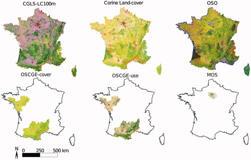
From the analysis of the state of the art, we propose to train a neural network to translate simultaneously multiple LULC maps in a multi-task manner. To do so, we first introduce the multi-LULC data set used for training. Experiments are carried out on the full Metropolitan French territory (mainland plus Corsica island), encompassing numerous landscapes: waterfronts, mountains, wetlands, forests, urban and agricultural zones. To extensively study LULC translation, we selected six open access LULC maps, exhibiting various production methods (either photo-interpreted or automatically generated), spatial resolutions (from 10 to 100 m), nomenclatures (from 11 to 44 classes, cover and use) and spatial extent (from 10,000 to 500,000 km²). In this section, we first focus on their main characteristics. Second, we detail the pre-processing steps and the corresponding manually built ground truth designed for quality assessment. This multi land-use/land-cover data-set (MLULC) (Baudoux 2022) is made available at https://doi.org/10.5281/zenodo.5843595.

3.1. Presentation of the input LULC

Among all the LULC covering France, we selected six maps that cover a broad range of specifications while ensuring at least a 70% overall accuracy: CGLS-LC100 (Buchhorn et al. 2020), CORINE Land Cover (Moiret-Guigand et al. 2021), OSO (Inglada et al. 2017), OCS-GE cover, OCS-GE use, and MOS. Table 1 summarises the main characteristics of each of these maps. They are described below.

Table 1. Main characteristics of the six selected LULC maps.

	CGLS-LC100 (Buchhorn et al. 2020)	CLC (Moiret-Guigand et al. 2021)	OSO (Inglada et al. 2017)	OCS-GE cover (OCS 2016)	OCS-GE use (OCS 2016)	MOS
Extent	World	Europe	France	West and South France	West and South France	Paris area
Generation	Machine learning	Photo-interpreted	Machine learning	Photo-interpreted	Photo-interpreted	Photo-interpreted
Source data	PROBA-V	Landsat, Sentinel-2	Sentinel-2	Aerial imagery	Aerial imagery	Aerial imagery
Used format	raster	vector	raster	vector	vector	vector
Selected year	2018	2018	2018	2014–2015	2014–2015	2017
Number of classes	12	44	23	14	17	11
Raster spatial resolution (m)	100	100	10	10	10	20
Minimum mapping unit	10,000 m^2	250,000 m^2, 100 m width	100 m^2	200–2500 m^2	200–2500 m^2 width	400 m^2
Official geometric accuracy	100 m	100 m	10 m	5 m	5 m	5 m
Official semantic accuracy	73% (Europe)	92% (Europe)	87% (France)
Accuracy on our ground truth	80% (France)	88% (France)	86% (France)

The impact of changes occurring between two maps in the translation procedure is reduced by carefully selecting the year of the maps and make them the closest possible to each other (selected years are indicated in Table 1). Few maps are produced in a yearly basis which inevitably generates discrepancies between the six maps.

The Copernicus Global Land Service Land Cover (CGLS-LC100) map has global coverage and is released annually in raster format. Based on PROBA-V image time series classification with a supervised Random Forest framework (Buchhorn et al. 2020), each map covers a civil year reference period with five released versions so far (2015–2019). Main map characteristics include a spatial resolution of 100 m, up to 22 classes (with a fine-grained separation into 12 forest labels), and hierarchically organised into a 3 level nomenclature. Level 1 merges all forest classes into one (leading to 11 classes), and level 2 distinguishes open from closed forests. We choose to rely on the level 2 nomenclature (see Appendix A Table A6), instead of the level 3 due to its higher accuracy (estimated overall accuracy over Europe of 80% at level 1, 73% at level 2 and not communicated at level 3 (Tsendbazar et al. 2020)). Indeed, our proposed solution relies on a supervised learning process: inserting a too significant noise level would be detrimental (Natarajan et al. 2013). Moreover, working with level 3 labels would have also required to deal with complex classes such as Unknown open forest types that cannot be correctly handled by any translation system.

The CORINE LULC (CLC) database and its 92+% thematic accuracy (Moiret-Guigand et al. 2021) has been the reference for land-use and land-cover documentation at the European scale for the last three decades. Five versions of the product have been released (1990, 2000, 2006, 2012 and 2018), covering up to 39 countries in 2018. CLC is mainly generated through visual inspection of both mono and multi-temporal (very) high-resolution optical satellite images (Landsat, Sentinel-2, SPOT), complemented with local databases. CLC is released dually in vector format with a 250,000 m² minimum mapping unit (MMU) for classes represented by polygonal objects and an additional 100 m width constraint for linear features, and in raster format with a 100 × 100 m pixel spatial resolution. The nomenclature includes up to 44 classes (Appendix A Table A1), hierarchically organised into a 3-level nomenclature. Since translation accuracy highly depends on the semantic and spatial correspondences between the source and the desired nomenclatures, a frequent method is to decrease the number of classes, focusing only on five to ten classes in the target map (Bechtel et al. 2020)). In the following, we target full CLC level 3 translation (44 classes) in order to better understand and assess which classes can be distinguished using contextual methods. Indeed, context-based translation solutions exhibit a significant potential for some challenging CLC level 3 classes (e.g. Mixed Forest, or Green urban areas) that calls for fine assessment.

The Occupation des Sols Opérationnelle (OSO) covers Metropolitan France and is released annually in raster format. Based on Sentinel-2 image time series classification with a supervised Random Forest framework (Inglada et al. 2017), each map covers a civil year reference period with five released versions so far (2016–2020). Main map characteristics include a spatial resolution of 10 m, 23 classes with a fine-grained 11 agricultural discrimination (see Appendix A Table A2), and an overall accuracy higher than 85%. This product is valuable to this study for its high resolution coupled with a detailed crop nomenclature. The OSO product is freely distributed around April each year (https://www.theia-land.fr/en/product/LULC-map/.

The Occupation des Sols à Grande Echelle (OCS-GE) map covers West and South-West France (125,000 km²), and is expected to be updated at least on a 5-year basis. Based on photo-interpretation of aerial visible and near infrared imagery, each administrative state is mapped independently with a first campaign between 2014 and 2015 and one between 2020 and 2021. Our work only includes 2014–2015 maps, the more recent one still being under review. Main map characteristics include a spatial class-dependent resolution between 5 and 10 m, a MMU between 200 and 2500 m² depending on the class and the location and two land-cover/land-user nomenclatures: 14 labels for land-cover (see Appendix A Table A4) and 17 for land-use. This joint LC/LU product is particularly interesting to study automatic land-use prediction from land-cover (so far, both are generated on the same spatial support but with two distinct steps). In the remainder, we will refer to those two nomenclatures as OCS-GEc for land-cover and OCS-GEu for land-use. The choice has been made to remove the following three classes from OCS-GEu: Other primary productions, Other transport networks and Unknown use, due to their mixed and ambiguously defined content.

The Mode d’Occupation des Sols (MOS) map covers the Paris region (12,000 km²) and is released approximately every 4 years in vector format. Based on the visual interpretation of 0.15 m aerial optical imagery, each map covers a civil year reference period with nine released versions so far (1982, 1987, 1990, 1994, 1999, 2003, 2008, 2012 and 2017). Main map characteristics include a spatial resolution around 20 m, up to 81 classes (with a fine-grained 68 built-up classes), hierarchically organised into a 4-level nomenclature. The choice to rely only on the 11 class level 1 nomenclature (see Appendix A Table A3) has been made since the other levels are not freely available.

3.2. Building a translation data set

The translation data set is generated according to the procedure described below:

1. Maps are downloaded from their respective official websites. Vector format is always chosen when available to reduce re-projection deformations.

2. Each map is cropped and aligned according to France borders.

3. The maps are then re-projected to the French official projection system ESPG:2154. This step involves nearest neighbour resampling for maps only available in raster format enforcing to preserve the original resolution. This step produces a spatial shift for those raster maps with a degradation of the geometric resolution that can reach the size of one pixel.

4. Vector maps are rasterised following their respective resolutions.

5. The maps are cropped into tiles of 6 × 6 km² to be ingested in our framework.

6. The tiles are dispatched in three sets: train (60%), validation (5%) and test (35%).

Since several maps do not cover the full French territory, the number of available maps varies, depending on the considered location, as shown in Figure 2. This is particularly interesting to study the generalisation to unseen areas and the previously mentioned impact of the unbalance in data set sizes in multi-task learning.

Figure 2. Spatial extent of the six land-cover maps used in this work. The color codes describing the classes of each map are provided in Appendix A.

3.3. Quality assessment

Three different evaluation approaches are introduced in this work: the comparison between our translation and (1) the original LULC; (2) 2300 random samples of manually annotated ground truth; (3) the latter ground truth enriched with 400 additional manually annotated samples focusing on rare labels. Table 2 summarises the main characteristics of the three evaluation data sets used.

Table 2. Summary of the characteristics of the three data-sets used for translation evaluation.

Evaluation data	Target map	Random ground truth	Enriched ground truth
Sample size	>100,000 for all LULC	2300	2300 + 400
Minimum sample per class	>1000	0	10
Pros	- Huge sample	- France wide coverage for all maps	- France wide coverage for all maps
Cons	- Same errors as target data - Only covers the target extent	- Small minimum sample per class	- Partially biased to increase sample size of rare classes
Usage	- Overall accuracy - Per class accuracy	- Overall accuracy - Generalisation	- Per class accuracy - Generalisation

Comparison between translated and target maps is the simplest way to assess the quality of the translation. However, since LULC maps contain errors, this measure is maximised when the translation exhibits the same errors as the target data. Therefore, we refer to this comparison as an agreement measure rather than an accuracy measure. Since comparison can be performed pixel-wise all over our test set, this comparison offers a vast number of samples per class, leading to an imperfect proxy to evaluate absolute and per-class metrics. It is worth noting that the agreement measure can only be computed on each LULC map extent. For instance, when studying the translation from MOS to OSO, the agreement between the translation output and OSO can only be computed on the spatial support of MOS (Paris area). In contrast, the CLC-to-OSO translation can be computed over full France. To sum up, the comparison between translation and target is useful to estimate per-class metrics but does not allow to detect if the method learns to replicate target errors. However, it does not allow studying generalisation to wider spatial extents.

Conversely, the comparison with an independent ground truth gives a better estimate of the accuracy. However, creating such a ground truth on each specific map spatial extent for all of the six maps with enough points to compute significant per-class accuracies (Foody 2002) is unrealistic for both time and lack of expertise reasons. This ground truth should be country-wide (to study generalisation to wider spatial extents) and with classes compliant with the specifications of each map.

To define a suitable sample size n for the ground truth we rely on Equation (1)(1) $$n=\frac{z^2\alpha (1-\alpha )}{m^2},$$(1) (Cochran 1977, Olofsson et al. 2014): (1) $$n=\frac{z^2\alpha (1-\alpha )}{m^2},$$(1) where z is a percentile from the standard normal distribution, α is the overall accuracy and m is the margin of error. For z = 1.96 (for a 95% confidence interval), $\alpha =50\%$ (worst case scenario) and $m=2\%,$ we obtained a target sample size of n = 2300.

These 2300 points are randomly sampled from the test set: they cannot be used to compute per-class accuracy due to the low (or null) number of samples for rare classes. We also provide 400 additional points (non-randomly sampled), focusing on rare classes to ensure a minimum of 15 points per class. Since most of these additional points were added to complete some of the 44 CLC classes, they abide by the 25 ha MMU of CLC. This significantly affects statistics for other maps (i.e. most CLC Sport and leisure facilities included points were golfs since they cover large surfaces and subsequently artificially enriches the MOS Artificial green urban areas with numerous golfs). The points in the ground truth are sampled with a minimum distance of 2.5 km to reduce spatial correlation. However, the MMU of CLC on linear elements does not guarantee independence below this distance.

Ground truth labelling relies on photo-interpretation of Sentinel-2 imagery and two independent sources of information: (i) the French authoritative cartographic database (BD Topo), yearly updated at 2 m with more than a hundred classes and (ii) the national Land Parcel Information System (Registre Parcellaire Graphique [RPG]), a 10 m farmers declarative database for European Common Agricultural Policy (CAP) (Cantelaube and Carles 2014). We consider the target data valid unless it disagrees with those sets, in which case photo-interpretation is performed.

The ground truth is partially biased for two reasons. First, the two databases only cover about 75% of France since some structures are excluded (e.g. sidewalks), and information is lacking (missing farmer declarations, especially for crops not included in CAP subsidies). The ground truth for some classes cannot be obtained. Secondly, the generated ground truth is a partially corrected version of the original data instead of a completely independent ground truth (i.e. favourably biased towards the original data). We refer to this measure to ‘accuracy’ hereafter.

4. Methods

This section presents our method to translate each map of a given set of LULC maps into another one of this set (applied to the case of six examples). The full implementation is made available at https://doi.org/10.5281/zenodo.7019838. We propose a supervised approach that learns to simultaneously transform the spatial resolution and the nomenclature of our six maps. Our method relies on CNN, with a standard encoder-decoder strategy, for their outstanding performance in jointly fostering information extraction from the semantic and spatial domains (Xing et al. 2020).

4.1. An encoder-decoder architecture

We aim to find a generic, simultaneous transformation of the nomenclature and spatial resolution of our six maps. Inspired by the existing literature, we enforce the translation to use a intermediate common representation space for all maps. This representation will be referred as an ‘embedding’ which we define as a heuristic model of land cover independent of a legend or resolution (within a limit of the six training maps). This leads to reach two consecutive objectives: (1) project each map into a shared embedding space; (2) decode this embedding into each one of our maps.

Based on recent works on multi-modal data representation (Chakravarty et al. 2019, Huang et al. 2020, Jo et al. 2020, Yu et al. 2020, Xing et al. 2021), we propose to train separate encoders and decoders for each map, and subsequently use cross-reconstruction to enforce common representations of similar land use/land cover (see Figure 3). We train our network to both reconstruct a given LULC with one decoder and to translate into the desired target LULC with another decoder. This dual objective enforces the embedding to be rich enough to preserve all source map information (reconstruction) while encoding it suitably for translation. Even though cross-reconstruction encourages the learnt embedding to be comparable for all LULC, it does not guarantee it. Therefore, multiple works also included a constraint on embedding pairs of corresponding data (e.g. using adversarial training or a loss term for embedding comparison). We adopt the latter strategy by computing the Mean Square Error between embeddings covering the same spatial extent.

Figure 3. The proposed cross-encoder architecture. In purple and green, two LULC maps with respectively c₁ and c₂ classes and $r_1\times r_1$ and $r_2\times r_2$ pixels. We represent in orange the common embedding space.

Instead of computing the loss for all maps covering one spatial extent, the network is trained by computing the loss for only one pair of maps at each optimisation step. This pair-wise optimisation is used as a workaround for GPU memory limitations. LULC translation requires large image patches to account for the MMU of some maps. In parallel, simultaneously training multiple networks is memory consuming. This scheme enables larger batches and achieves a better result than optimising all different maps simultaneously on smaller batches. This iterative pair-wise approach is also the one generally used in multi-lingual model training (Conneau et al. 2020). In practice, at each optimiser step, we compute the loss for one pair of maps using Equation (2)(2) $$L=L_{\mathit{rec}}+L_{\mathit{tra}}+L_{\mathit{emb}}.$$(2) . (2) $$L=L_{\mathit{rec}}+L_{\mathit{tra}}+L_{\mathit{emb}}.$$(2)

L_rec is the reconstruction loss used to enforce the embedding to maintain all information specific to each LULC, computed as the sum of two cross-entropies between the two self-reconstructed and their respective sources. L_tra evaluates the quality of the translation and is computed as the sum of the two cross-entropies of the two translated maps and their respective targets. L_emb is the MSE loss between the embedding of the two source maps which enforces the representation to be shared between LULC. The global loss is theoretically minimal when the three following assumptions are met simultaneously: (1) the self-reconstruction of each map is perfect; (2) the translation is also perfect; (3) embeddings on the same areas are identical.

Our previous work showed that geographical coordinates can be effectively inserted to improve translation using a positional encoding strategy (Baudoux et al. 2021). Following this observation, we adopt this principle by adding a geographical coordinate sub-module to our encoder.

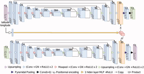
4.2. Network architecture

The design of our MLCT-Net is made according to the following observations:

1. The encoder must have a sufficient receptive field to encode each object using its surroundings. Thus, the architecture is constrained by the MMU of each map. Since CLC has a 250,000 m² MMU, the receptive field should at least have a 250,000 m² width. An embedding with ground resolution of 10 m per pixel leads to at least a 250 pixel-wide receptive field.

2. The decoder should remain as simple as possible to ensure that the learnt embedding remains as identical as possible for all LULC. Decoders with high capacity may lead to a latent space with small information content.

We develop the architecture illustrated in Figure 3. It is mainly composed, for each map, of a (1) a nearest neighbour resampling to the highest spatial resolution (10 m), (2) a U-Net (Ronneberger et al. 2015) encoder, (3) and a spatial pyramidal pooling (Chen et al. 2018) followed by a 1-pixel wide kernel convolution layer as a decoder. This architecture meets each of the above criteria. The 10 m resampling strategy enables the use of the same architecture for each map. This strategy only works if the gap between the lowest and the highest LULC resolutions remains limited: a low resolution enforces the LULC patches to cover a wide area to get a grasp of the spatial context. This results in very large patches for the maps with higher resolutions. The U-Net deals with the receptive field size by down-sampling the input multiple times, which is more memory efficient than increasing the network depth. There are only two differences with respect to the original U-Net architecture. The first one is the use of Group Normalisation (Wu and He 2018) instead of Batch Normalisation leading to stable normalisation, even on small batch sizes. The second one is the use of five down-sampling blocks, instead of four, to widen the receptive field.

Data augmentation in the training procedure by randomly rotating and flipping the maps limits overfitting. This strategy is particularly beneficial on the MOS map, which only includes around 250 patches for training.

4.3. Geographical context encoding

Based on the observation that LULC translation might depend on the geographical location (a tree might be translated differently if located near water areas or on a mountain), we used the same geographical encoding strategy as in Baudoux et al. (2021). For each patch, we transform the geographical coordinates into pixel coordinates following (Parmar et al. 2018), which mainly consists in a 2D adaptation of the positional encoding of Vaswani et al. (2017). Positional encoding, in natural language processing, encodes the position of each word to tackle issues fostered by differences between the number of words in the sentences of the training and testing set (i.e. you trained only on sentences with less than 20 words and then there is on sentence with 21 one words in inference). The same problem arises in our geographical context encoding setup, as the coordinates of the training and testing sets are different. The positional encoding mechanism notably improves the spatial generalization ability when your training and testing spatial coordinates are not the same (Mai et al., 2022). For a given longitude x and latitude y, the positional encoded matrix $p_{x,y}$ of dimension d (in our setup d = 128) is given by Equation (3)(3) $$p_x={\left[\begin{array}{c}\hspace{0.17em}\mathit{sin}\hspace{0.17em}(x{\omega }_1)\\ \hspace{0.17em}\mathit{cos}\hspace{0.17em}(x{\omega }_1)\\ ⋮\\ \hspace{0.17em}\mathit{sin}\hspace{0.17em}(x{\omega }_{d/4})\\ \hspace{0.17em}\mathit{cos}\hspace{0.17em}(x{\omega }_{d/4})\end{array}\right]}_{d/2}\mathrm{ }{p}_y={\left[\begin{array}{c}\hspace{0.17em}\mathit{sin}\hspace{0.17em}(y{\omega }_1)\\ \hspace{0.17em}\mathit{cos}\hspace{0.17em}(y{\omega }_1)\\ ⋮\\ \hspace{0.17em}\mathit{sin}\hspace{0.17em}(y{\omega }_{d/4})\\ \hspace{0.17em}\mathit{cos}\hspace{0.17em}(y{\omega }_{d/4})\end{array}\right]}_{d/2}\mathrm{ }{p}_{x,y}={\left[\begin{array}{c}\hspace{0.17em}\mathit{sin}\hspace{0.17em}(x{\omega }_1)\\ \hspace{0.17em}\mathit{cos}\hspace{0.17em}(x{\omega }_1)\\ ⋮\\ \hspace{0.17em}\mathit{sin}\hspace{0.17em}(y{\omega }_{d/4})\\ \hspace{0.17em}\mathit{cos}\hspace{0.17em}(y{\omega }_{d/4})\end{array}\right]}_{d}w\mathit{ith}{\omega }_i=\frac{1}{{10000}^{2i/d}}$$(3) : (3) $$p_x={\left[\begin{array}{c}\hspace{0.17em}\mathit{sin}\hspace{0.17em}(x{\omega }_1)\\ \hspace{0.17em}\mathit{cos}\hspace{0.17em}(x{\omega }_1)\\ ⋮\\ \hspace{0.17em}\mathit{sin}\hspace{0.17em}(x{\omega }_{d/4})\\ \hspace{0.17em}\mathit{cos}\hspace{0.17em}(x{\omega }_{d/4})\end{array}\right]}_{d/2}\mathrm{ }{p}_y={\left[\begin{array}{c}\hspace{0.17em}\mathit{sin}\hspace{0.17em}(y{\omega }_1)\\ \hspace{0.17em}\mathit{cos}\hspace{0.17em}(y{\omega }_1)\\ ⋮\\ \hspace{0.17em}\mathit{sin}\hspace{0.17em}(y{\omega }_{d/4})\\ \hspace{0.17em}\mathit{cos}\hspace{0.17em}(y{\omega }_{d/4})\end{array}\right]}_{d/2}\mathrm{ }{p}_{x,y}={\left[\begin{array}{c}\hspace{0.17em}\mathit{sin}\hspace{0.17em}(x{\omega }_1)\\ \hspace{0.17em}\mathit{cos}\hspace{0.17em}(x{\omega }_1)\\ ⋮\\ \hspace{0.17em}\mathit{sin}\hspace{0.17em}(y{\omega }_{d/4})\\ \hspace{0.17em}\mathit{cos}\hspace{0.17em}(y{\omega }_{d/4})\end{array}\right]}_{d}w\mathit{ith}{\omega }_i=\frac{1}{{10000}^{2i/d}}$$(3)

After encoding through a single hidden layer multi-layer perceptron (MLP) and a softmax layer, we multiply the geographical context representation by the embedding of each map (Figure 3). The choice of a softmax followed by a multiplication over a simple addition mainly relies on the willingness to maintain generalisation ability on spatial extents unseen during training.

Each translation does not necessarily need the same geographical context information. One could then learn one context per pair-wise translation. However, it would be impossible to generalise the translation to an area of the target map extent used during training. For example, learning a specific geographical context for the OSO-to-MOS translation is only possible on the spatial extent shared by the two maps and not outside. To preserve the common representation space of the embedding, we train a unique MLP on the set of coordinates of our patches. This specific geographical context representation slightly worsens the translation quality, compared to learning a per-translation representation. However, it remains the only valid strategy.

4.4. Comparison baselines

To the best of our knowledge, no other multi-LULC translation method has been published. We, therefore, compare our approach to three mono-LULC translation methods.

4.4.1. Semantic baseline

A rule-based semantic translation where the bijective association between each source and each target class is manually defined. Associations are detailed for each LULC in Appendix A. The semantic association is followed by a spatial resampling. When the target spatial resolution is finer than the source one, a nearest neighbour up-sampling is performed. Conversely, a majority voting rule is applied for down-sampling. This method enables to compare rule-based semantic translations with data-driven ones.

4.4.2. Statistical baseline

A statistical matching between source and target classes. We first compute the probability of a source class to be translated into each target map using the available training set. When the spatial resolution of the target is similar or finer than the source, we attribute to each source class the most probable target class. When the spatial resolution of the target is coarser than the source, we compute inside each target pixel the mean of the probability for each source pixel to be translated in each target class. This results in an adaptation of the majority voting resampling used in the semantic baseline. This method is used to compare data-driven methods unaware of the spatial context with context-wise ones.

4.4.3. Mono-LULC contextual translation

An asymmetrical U-Net augmented with a geographical context module for taking spatial context into account during a pairwise translation (Baudoux et al. 2021). This method is used to study the benefit of learning a multi-LULC translation over a mono-LULC, simpler case.

Results provided by MLCT-Net are expected to be better than with the two first methods. They should be at least on par with the mono-LULC translation method, and better on LULC with few training patches, as observed in natural language processing.

5. Results

In this section, we investigate the translating power of our method and evaluate the effect of learning a multi-LULC translation instead of a standard mono-LULC procedure. The experimental set-up and the various experiments are subsequently detailed.

5.1. Evaluation metrics

Quantitative evaluation is performed through Overall Accuracy computation to account for global quality. LULC data sets are highly class-imbalanced: high accuracy can be achieved by simply correctly predicting the most frequent classes (often not the most difficult to discriminate). We compute the macro f1-score to more accurately assess the quality of the translated classes. Standard per-class metrics (precision, recall and f1-score) are also computed. Formulas for per-class metrics and overall metrics are given in Equations (4)(4) $$p_i=\sum _{j=1}^c\frac{m_{ii}}{m_{ji}},r_i=\sum _{j=1}^c\frac{m_{ii}}{m_{ij}},F{1}_i=\sum _{j=1}^{c}2\frac{p_i{r}_i}{p_i+r_i},$$(4) and (5)(5) $$OA=\frac{\sum _{i=1}^c{m}_{ii}}{\sum _{i,j=1}^c{m}_{ij}},mF1=\frac{1}{n}\sum _{j=1}^{c}F{1}_i.$$(5) , respectively. (4) $$p_i=\sum _{j=1}^c\frac{m_{ii}}{m_{ji}},r_i=\sum _{j=1}^c\frac{m_{ii}}{m_{ij}},F{1}_i=\sum _{j=1}^{c}2\frac{p_i{r}_i}{p_i+r_i},$$(4) (5) $$OA=\frac{\sum _{i=1}^c{m}_{ii}}{\sum _{i,j=1}^c{m}_{ij}},mF1=\frac{1}{n}\sum _{j=1}^{c}F{1}_i.$$(5) p_i, r_i and $F{1}_i$ are the precision, recall, and f-score for a given class i, respectively. OA is the overall accuracy, mF1 is the macro f1-score, c is the number of classes, and m_ij is the element in the jth row of the ith column of the confusion matrix, i.e. the number of pixels of class j classified as i. These statistics are computed separately by comparing the translation with (a) the target LULC, and (b) the ground truth.

5.2. Qualitative assessment

Beyond quantitative metrics, visual inspection of land-cover maps is useful to understand the behaviour of the algorithms. The colour codes of each LULC map are provided in Appendix A.

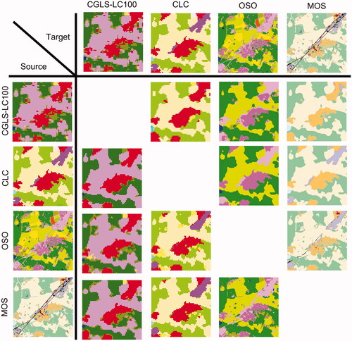
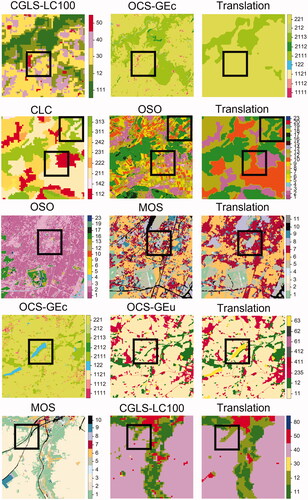
Figure 4 presents the results of the 12 translation results obtained on a patch of the Paris area. Each row corresponds to the translation of one source map into the four other ones available for this area. Unsurprisingly, one can first note that coarse-to-high resolution translation with our approach results in almost similar performance than a semantic rule-based approach associating one unique target class to each source class. This is due to the limited spatial and semantic information in such LULC maps (e.g. CORINE Land Cover). External data (satellite imagery) could participate in increasing the translation performances. The second observation is that our network may face some difficulties in learning the MMU of CLC (here 25 pixels) as shown by the small three pixel wide urban areas in Figure 4 (in red, first column). Commonly, network training leads to replicate in the predictions the bias observed in the original data. The most striking example is OSO road class, which has a 45% recall in the original data. It is often confused with Industrial and commercial units (ICU). When learning to translate a road from a given LULC source map to the OSO map, the corresponding class has a high probability of being an OSO ICU (e.g. MOS-OSO translation case in Figure 4, 3rd row, 2nd column). This also increases the difficulty in quantitatively assessing the quality of the results using the target data as reference.

Figure 4. MLCT-Net translation results for all source/target LULC maps pairs available on a 6 × 6 km² patch of the Paris area.

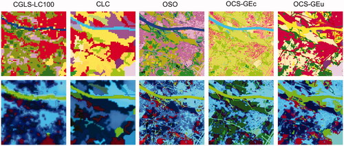
Figure 5 presents a set of patches selected for their representativeness of the behaviour of MLCT-Net. The first observation is that the spatial context influences the translation mainly on object edges, especially when the source exhibits a low resolution. In the first row, the border of a CLC Discontinuous urban area is translated into an OSO pasture area. Second, when the gap between spatial resolutions remains limited, the translation achieves a successful context-dependent translation (i.e. the same class is translated differently according to its neighbourhood), as shown for example in Figure 5 (second row): OSO sparse urban and ICU are satisfactorily translated into either MOS Individual housing, Collective housing or Activity areas, based on each source class density or, on the third row, where MOS Forest is translated into CGLS-LC100 Open forest or Closed forest, thanks to the elongated shape of the object. The third observation is that, despite context, some translation cases remain difficult. Additional external data could for example be used in the fifth row where an OCS-GEc Water area must be translated into it is land-use counterpart. Most of the time, such areas are classified as No-use in OSC-GEu. However, in this case, this water lake is used for farming which the network fails to predict. This difficult case illustrates the limitation of MLCT-Net: despite higher scores related to spatial context insertion, it is still insufficient to achieve to perfect translation.

Figure 5. Benefits and limitations of multi-LULC map translation. Each square highlights an area with meaningful spatial context (see text for more details).

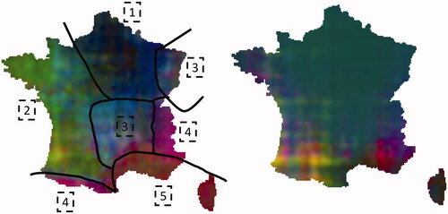
To assess if our LULC maps are all correctly embedded in a shared representation space, we provide Figure 6 which presents the embedding of one patch for five different maps. The 3-channel representation of the embeddings stems from a PCA on the original 30-dimension embeddings using a random subset of 1% of the embedding of the train set. All are rather similar, which was expected through the double constraint of cross-reconstruction and the MSE computation between embeddings. Second, edges have a particular behaviour in the embeddings. This is particularly visible on coarse resolution maps (such as CLC) with a gradient on each object near the edges. It can easily be explained by a higher uncertainty of the translation near object boundaries. The third observation is that the learnt embedding for coarse resolution maps has a blurrier aspect than high-resolution ones (e.g. in the CGLS-LC100 embedding, especially on Built up areas). We relate this behaviour to the relative uncertainty of the semantic content of an area on a low-resolution map compared to a higher-resolution one (i.e. a Built up area might simultaneously include trees, dense or sparse urban, and roads). Close values in the embedding space for two classes often reflect close semantic values: all artificial surfaces, like roads or buildings appear in light blue, all forest types (coniferous, broad-leaved) in light to strong red, all sorts of crops and pastures in dark blue. This closeness might be beneficial for tasks such as zero-shot learning since semantically close elements are represented closely in our embedding space. Eventually, when one class of a LULC map establishes a complex semantic relationship with another map, it is often visible in the embedding. For example, the OSC-GE cover class Herbaceous vegetation mixes cultivated areas and natural grasslands while all other maps make a clear distinction between those two vegetation types. This leads to distinct embeddings (green ↔ dark blue).

Figure 6. Shared embeddings (below) for five LULC maps of interest (top). Colors result from a dimension reduction from the original 30-dimension embedding to 3 dimensions (RGB) using Principal Component Analysis.

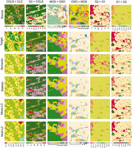
5.3. Quantitative assessment and comparison with other methods

All conceivable translation scenarios using our method were tested, fed with the six maps. We also evaluated the three baselines mentioned in Section 4.4. Table 3 reports the agreement between all translations and each LULC map. Note that the agreement can only be computed on the target spatial extent (i.e. the agreement is computed on the Paris area (2% of France surface) when MOS is the target, country-wide when CLC is the target).

Table 3. Agreement between our translation and the original target maps. P: CGLS-LC100, C: CLC, O: OSO, G1: OCS-GEc, G2: OCS-GEu, M: MOS.

Source		P					C					O					G1				G2				M
Target		C	O	G1	G2	M	P	O	G1	G2	M	P	C	G1	G2	M	P	C	O	G2	P	C	O	G1	P	C	O
OA	semantic	52	42	56	70	75	65	49	67	77	79	62	59	69	76	81	56	41	34	87	57	40	31	75	80	76	59
	statistic	54	44	65	70	75	68	55	71	78	79	65	61	73	80	82	57	44	49	89	57	40	41	78	83	81	62
	mono-LC	64	57	69	78	76	74	59	72	80	80	77	69	80	86	85	71	58	58	93	69	54	53	79	85	83	63
	multi-LC	64	56	69	78	77	74	59	72	81	80	76	66	78	86	85	70	58	58	92	69	54	53	80	86	84	64
mF1	semantic	13	17	22	15	24	46	26	36	28	42	38	19	36	20	38	27	10	17	27	20	9	8	29	38	19	19
	statistic	13	18	19	16	24	47	32	33	30	42	36	18	34	20	39	27	10	20	27	20	9	10	27	32	17	18
	mono-LC	30	33	29	20	31	57	37	36	31	41	61	39	45	26	53	52	34	31	43	52	29	25	40	45	30	23
	multi-LC	30	29	30	19	34	59	35	37	26	41	56	36	43	23	52	50	34	32	37	49	30	26	43	48	36	23

Best values are displayed in bold.

First, context-aware translation methods have higher agreements than their semantic and statistical counterparts. The improvement between contextual and non-contextual methods ranges from 1% to 17%. The smallest differences are usually observed when the source map has a coarser spatial resolution than the target. It is impossible to obtain high scores on a spatial super-resolution task without adding fine geometric and spatial information (e.g. very high-resolution images). In practice, a good rule of thumb is to estimate that the MMU of the target maps is always of the same magnitude than the source one (i.e. translation a 25 ha MMU LULC results in a more or less 25 ha MMU). Conversely, significantly better results are observed when a high-resolution map is translated into a coarser one.

Figure 7 presents the qualitative comparison of Statistic, Semantic, Mono-LC and MLCT-Net on the same spatial extents. A first observation is that mono-LULC and MLCT-Net methods outperform the semantic and statistic baselines when source classes have multiple probable translations. For instance, for OSCGEuse (G2)-to-CGLS translation, ‘Agriculture areas’ are translated solely into ‘croplands’ by the semantic method while being translated quite accurately both into cropland and pastures by the context-aware methods. The same observation holds for urban areas in the OSCEuse-to-OCS-GEc translation (and OCS-GEc-to-OCS-GEu). A second observation is that pure semantic-based translation outperforms other methods on erroneous classes in the original target data. For MOS-to-OSO translation, roads (black on the MOS map) are always translated into ICU except by the semantic baseline. This behaviour is learnt from the original OSO map, which often presents this confusion. Conversely, the learnt methods outperform the semantic baseline when the source map is erroneous. In the reverse translation case (from OSO to MOS), the erroneous ICU (truth: roads) are correctly translated into roads in the MOS maps by all methods except the semantic one.

Figure 7. Visual comparison between the output of MLCT-Net and existing baselines.

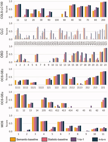
The analysis of the differences in terms of macro f1-score is also highly informative: mono and multi-LULC translations successfully use spatial context to significantly outperform the simpler counterparts, in terms of number of predicted classes (exception made of the CLC-to-OCS-GEu configuration, mostly due to the difficulty to translate the OCS-GEu No-use class). To get a better understanding of which classes are predictable, we provide the observed per-class f1-score in Figure 8. Since displaying all the 26 possible configurations would be counterproductive, we added the confusion matrices of all maps for each target LULC, resulting in one confusion matrix per target map. We computed the per-class f1-score, i.e. CLC per-class f1-score is computed on the merged confusion matrix of OSO-to-CLC, MOS-to-CLC, PROBA-to-CLC, OCS-GEc-to-CLC and OCS-GEu-to-CLC. Therefore, in Figure 8, a high f1-score is reached when the translation from all sources to the considered target is successful. We can state that the well-predicted classes are identical for all methods. The translation into CLC is the one for which context-wise methods are the most beneficial, as it significantly increases the number of partially predictable classes, compared to the semantic and statistical baselines. In other cases, the insertion of context mainly helps to improve translation on specific classes, especially those defined by a spatial pattern such as CLC Heterogeneous crops (mix between arable and permanent crops), and on spatially correlated classes. Forests in mountainous areas mainly include coniferous stands. Thus, a forest in this area is more likely to be translated as Coniferous than Broad-leaved).

Figure 8. Per-class F1 agreement computed on the sum of the translation confusion matrices of all the sources to one target.

Our multi-LULC approach has a similar agreement to the mono-LULC scenario, exhibiting close scores in most cases. However, one must note that it tends to slightly under-perform on the OSO-any other configuration. MLCT-Net tends to have more difficulties in learning the MMU than the mono-LULC counterpart. Indeed, as mentioned previously, this behaviour is particularly striking in the case of the OSO-to-CLC translation, as shown in Figure 7. This observation is comforted by noticing that the mean area of errors in the multi-LULC model is significantly smaller than the mono-LULC model. This can be partly explained by the difficulty in learning the concept of MMU in a shared representation space, due to the risk of also applying the same MMU when translating finer resolution LULC maps. One could argue that learning the MMU only requires estimating the area occupied by classes and filtering non-adequate small areas. However, this would overlook that estimating areas is not a trivial task for a network fed with image patches, due to the lack of information on edges (ideally, this would require processing the whole data at once, which is unfeasible). Furthermore, undetected areas in the target data act like a deletion operator used in a generalisation procedure. While this last statements affect both multi-LULC and mono-LULC models, the difficulty in learning the MMU naturally increases as the number of generalisation rules (and errors) increases, explaining the poorer MMU learning of the multi-LULC model compared to its mono-LULC counterpart. Since OSO is the highest resolution map used in this study, translation from OSO are the most prone to MMU errors explaining the observed slight under-performance compared to the mono-LULC model.

5.4. LULC map extension

The generalisation ability of a deep neural network is a key feature when studying the representativeness of the shared space and subsequently the ‘universality’ of such learnt representation. A universal representation should be able to generalise learnt LULC maps to areas they do not originally cover. Such an extension ability is highly valuable. This would allow to generate only high-quality LULC maps on a restricted area without spending too much time to ensure country-wide generation.

To this extent, we propose to evaluate our ability to retrieve the target MOS, OCS-GEc and OCS-GEu over France from the sources OSO, CLC and PROBA-V LULC maps, while the three target LULC maps have only been produced over less than 20% of the country (down to 3% for MOS). To do so, each source map (OSO, CLC and CGLS-LC100) is translated into one of the targets at a France-wide scale. The translation may face unseen classes during training in both source and target maps (e.g. there is no glacier on the original MOS spatial extent) resulting in wrong translations. Therefore, for each pair of source/target maps, the semantic baseline is used to translate source classes unseen during training. Unseen target classes during training are ignored. OCS-GEc Snowfields and glaciers and Other non-woody formations are considered unseen due to high error of the OCS-GE data for those two classes. In this setup, mono-LULC models cannot be trained with the geographical coordinates sub-module since they are trained solely on the original target spatial extent. To assess if differences between the mono and multi-LULC models are due to the use of the geographical coordinates sub-module, we provide the multi-LULC results with and without it.

Table 4 presents the results computed on the 2300-point ground truth. We focus on the Overall Accuracy, such a limited number of measurements makes the f1-score unreliable. Conversely, Table 5 is used to evaluate the f1-score performances using the manually consolidated 2700 sample ground truth. Differences between our model and the baselines are significantly smaller than observed earlier for the agreement measure. This can be explained by two factors: (1) the ground truth is not fully representative of the French territory; (2) the network learnt to replicate some errors of the original maps, which increases the agreement. Our first observation is that MLCT-Net still outperforms the baselines even though the gap between these methods drastically decreases, both visually and compared to the gap observed on the agreement measurement. A detailed study on the failure cases reveals that this difference is mainly due to unseen objects during training. For example, sea areas are often confused with Forest instead of Water in the translated MOS maps, probably because there is no sea in the original MOS spatial extent. This observation holds for many classes that are not evenly spatially distributed, since they correspond to peculiar areas and topography (Salines and Glaciers). This underlines that semantic translation methods are more robust to generalisation than learnt ones, when confronted to totally new landscapes.

Table 4. Translation results for the 3 full France maps computed on our 2300 point ground truth. ‘no-c’ corresponds to ablation cases where the geographical coordinate sub-module is removed.

Source		P					C					O
Target		C	O	G1	G2	M	P	O	G1	G2	M	P	C	G1	G2	M
OA	Semantic	47	46	62	79	81	72	51	76	84	85	71	65	86	86	92
	Statistic	52	45	68	80	81	68	57	77	85	85	67	66	86	89	92
	Mono-LULC no c			70	82	76			78	86	78			86	91	87
	Mono-LULC	60	55				70	59				75	71
	Multi-LULC no c	57	52	71	83	82	71	59	78	86	86	78	70	87	91	93
	Multi-LULC	60	53	74	83	83	71	59	79	86	86	78	70	87	92	93
mF1	Semantic	15	19	26	24	26	50	34	44	46	41	44	24	47	29	44
	Statistic	15	19	23	28	26	57	35	38	47	39	39	22	43	31	43
	Mono-LULC no c			31	29	21			39	39	23			47	34	41
	Mono-LULC	28	27				57	37				58	43
	Multi-LULC no c	19	19	30	41	27	54	35	42	39	41	62	38	50	34	43
	Multi-LULC	28	22	34	41	29	58	33	43	44	38	63	37	50	35	44

Best values are displayed in bold.

Table 5. Translation results for the 3 full France maps computed on the consolidated 2700 point ground truth. ‘no-c’ corresponds to ablation cases where the geographical coordinate sub-module is removed.

Source		P					C					O
Target		C	O	G1	G2	M	P	O	G1	G2	M	P	C	G1	G2	M
OA	Semantic	43	45	60	72	74	71	52	74	82	83	68	60	83	80	86
	Statistic	48	43	64	75	74	67	56	75	84	82	63	60	82	85	86
	Mono-LULC no c			66	77	67			74	82	70			83	86	78
	Mono-LULC	55	53				66	56				71	68
	Multi-LULC no c	53	49	69	78	76	68	57	76	83	82	74	65	84	86	88
	Multi-LULC	56	50	70	79	77	68	57	77	83	82	74	65	85	87	87
mF1	Semantic	12	18	29	22	26	62	42	56	55	60	47	22	51	30	43
	Statistic	13	18	22	25	26	59	37	50	48	57	37	20	48	31	42
	Mono-LULC no c			31	26	22			45	42	38			53	34	39
	Mono-LULC	27	28				53	36				56	45
	Multi-LULC no c	21	18	33	27	29	57	34	51	41	55	58	34	57	32	48
	Multi-LULC	27	22	37	27	30	56	33	52	43	46	59	37	57	33	50

Best values are displayed in bold.

The multi-LULC model outperforms the mono-LULC model, especially in terms of f1-score. When translating to the MOS map, this stems from the coordinate sub-module (0.39 for mono-LULC with no coordinates, 0.48 for multi-LULC with no coordinates, 0.5 for multi-LULC with coordinates). This can easily be explained by the fact that the geographical context is most useful when translating unseen objects during training (such as sea). The smallest spatial extent maps (with lower diversity of classes and objects) benefit the most from the geographical context. On the contrary, the coordinate sub-module seems less useful on the two OCS-GE maps, which perform almost the same with and without it (larger and more diverse areas).

5.5. Ablation study

5.5.1. Geographical context encoding

Visualising the learnt geographical embedding is crucial to better understand its effect on the translation accuracy. Figure 9 compares such embeddings for the six map multi-LULC case and the mono-LULC case trained on the OSO-to-CLC translation. We applied a separate PCA on the output of the MLP module. We observe this encoding does not correlate with the number of maps or the nature of maps covering each area. Second, it seems that the encoding correlates well with major French geographical landscapes such as Alpes and Pyrenees mountains (pink), the Paris basin (blue), and the Mediterranean seashore (maroon). These results underline the representativeness of a learnt geographical encoding through a multi-LULC mapping and its suitability to improve results on classes correlated to unevenly spatially distributed landscapes. It is also interesting to compare those results with the geographical encoding obtained by a mono-LULC model. The mono-LULC model learns a specific geographical representation to compensate for local errors. In contrast, the multi-LULC models are more correlated to geographical information.

Figure 9. PCA representation of the learnt geographical context embedding for our multi-LULC model (left) and the mono-LULC OSO to CLC model (right). One may easily delineate the main French landscapes, namely (1) Paris basin, (2) Atlantic seacoast, (3) Medium mountains, (4) High mountains and (5) Mediterranean seashore.

5.5.2. Impact of the number of input LULC maps

We propose to analyse the influence of the number of maps fed into MLCT-Net and the quality of the translation. Figure 10 displays the accuracy depending on the number of maps used for learning. Each histogram represents the stacking of translation results from all maps towards a single one. The first histogram presents the average translation results of CLC, OSO, MOS, OCS-GEc and OCS-GEu in CGLS-LC100 for different models trained to perform mono-LC or multi-LC translation in using (2–6 maps). Error bars are computed as the mean of uncertainties estimated using Equation (6)(6) $$u(t)=\frac{1}{m}\sum _{s=1}^{m}z\sqrt{\frac{O{A}_s(1-O{A}_s)}{n}},$$(6) . (6) $$u(t)=\frac{1}{m}\sum _{s=1}^{m}z\sqrt{\frac{O{A}_s(1-O{A}_s)}{n}},$$(6) where u(t) is the uncertainty for a target map t, s is the considered source map, OA_s is the estimated accuracy of the translation from source s to map t, z = 1.96 for 95% confidence, n is the ground truth sample size (2,300), and m is the total of number of available source.

Figure 10. Mean accuracy per target land-cover for different models trained with one (mono-LULC) up to six maps. The red-dotted line separates LULC available France wide (left) from those with smaller spatial extent (right).

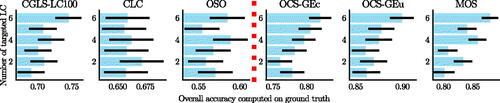
Although the model trained on six maps tends to perform better in the majority of cases, the performance variations observed on CGLS-LC100, CLC and OSO remain insignificant given the size of our ground truth. This statement prevents us from concluding on a real advantage of using a multi-LULC model for these three maps. This observation is further supported by the fact that there is no stable trend of a performance increase when going from 2 to 6 maps. On the other hand, a more straightforward and significant trend is observed on the MOS, OCS-GEc and OCS-GEu maps, which all initially covered only a fraction of the territory. The progressive increase comforts our previous analysis of greater robustness to generalisation to new landscapes of multi-LC models compared to the mono-LULC model.

6. Conclusion

In this article, we have comprehensively investigated the potential of country-wide multi-LULC map translation with our novel MLCT-Net model. In order to obtain a higher quality translation than models trained on specific pair-wise cases or non-spatial-context-aware existing methods, we inspired ourselves by recent work on multi-task and multi-modal deep learning models. Namely, we designed a multi-encoder decoder network incorporating a three-term loss: (1) a translation loss to evaluate the quality of the LULC translation, (2) a self-reconstruction loss to ensure that the embedding preserves each map information, (3) a maximum distance loss on the embedding to ensure that similar features of different maps are encoded the same way to ensure high-quality results even on unseen spatial extents. Each encoder is trained to project a specific map into a representation space shared between all LULC. Conversely, each decoder aims to translate this shared representation space into one target LULC. Our key contribution is such a universal country-wide representation space, which achieves an increase in translation generalization.

We comprehensively evaluated our method by comparing the obtained translations to the original LULC and a manually annotated ground truth. Our method outperforms the standard semantic and statistical methods that only focus on exploring per-class associations instead of defining context-aware solutions. The average improvement is about 9.5% in overall agreement between source and translation compared to the semantic baseline (6.2% for the statistical baseline). In contrast with the mono-LULC method, the multi-LULC method is only 0.4% worse in terms of overall agreement. Further statistics computed on our full France ground truth reveals that the multi-LULC model outperforms the mono-LULC when computing the translation of maps on a spatial extent that they do not initially cover. These results demonstrate that learning a universal representation for multiple LULC improves the robustness of the translation. We believe that the high potential of this spatial context-aware land-cover translation method might support new applications in inter-operating land-cover data sets. The method offers the advantage of generating maps with multiple variations of nomenclature and resolution without requiring remote sensing images. Therefore, it appears possible to use this land-cover translation for multiple downstream tasks such as change detection, updating, comparison or increasing the spatial extent of land-cover maps.

Data and codes availability statement

Data are made available at https://doi.org/10.5281/zenodo.5843595 and code at https://doi.org/10.5281/zenodo.7019838.

Disclosure statement

No potential conflict of interest was reported by the author(s).

Additional information

Funding

This work is funded by the MAESTRIA project [grant ANR-18-CE23-0023] and supported by the AI4GEO project http://www.ai4geo.eu/ and Agence Nationale de la Recherche.

Notes on contributors

Luc Baudoux

Luc Baudoux is a PhD candidate at the LASTIG and CESBIO laboratory at the Gustave Eiffel University in France. His research investigates how to increase land-cover quality and reusability.

Jordi Inglada

Jordi Inglada Jordi Inglada received the master’s degree in telecommunications engineering from the Universitat Politècnica de Catalunya, Barcelona, Spain, and the École Nationale Supérieure des Télécommunications de Bretagne, Brest, France, in 1997, and the Ph.D. degree in signalprocessing and telecommunications from the Université de Rennes 1, Rennes, France, in 2000. He is currently with the Centre National d’Etudes Spatiales (French Space Agency), Toulouse, France, where he is involved in the field of remote sensing image processing at the Centre d’Etudes Spatiales de la Biosphère (CESBIO) Laboratory. He is involved in the development of image processing algorithms for the operational exploitation of Earth observation images, mainly in the field of multitemporal image analysis for land use and cover change.

Clément Mallet

Clément Mallet is currently leading the LASTIG laboratory (Univ. Gustave Eiffel and French Mapping Agency) and is Editor-in-Chief of the ISPRS Journal of Photogrammetry and Remote Sensing. His main interests are land-cover mapping with remote sensing imagery and point cloud processing.

Appendix A.

Land cover nomenclatures

Table A1. CLC nomenclature.

THE main semantic link column gives for each CLC class the semantically closest class in the other LULC.

Table A2. OSO nomenclature.

The main semantic link column gives for each OSO class the semantically closest class in the other LULC.

Table A3. MOS nomenclature.

The main semantic link column gives for each MOS class the semantically closest class in the other LULC.

Table A4. OCS-GEc nomenclature.

The main semantic link column gives for each OCS-GEc class the semantically closest class in the other LULC.

Table A5. OCS-GEu nomenclature.

The main semantic link column gives for each OCS-GEu class the semantically closest class in the other LULC.

Table A6. CGLS-LC100 nomenclature.

The main semantic link column gives for each CGLS-LC100 class the semantically closest class in the other LULC.

References

- Adamo, M., et al., 2014. Expert knowledge for translating land cover/use maps to general habitat categories (GHC). Landscape Ecology, 29 (6), 1045–1067.
- Ahlqvist, O., 2005. Using uncertain conceptual spaces to translate between land cover categories. International Journal of Geographical Information Science, 19 (7), 831–857.
- Ahlqvist, O., 2008. In search of classification that supports the dynamics of science: the FAO land cover classification system and proposed modifications. Environment and Planning B, 35 (1), 169–186.
- Al-Mubaid, H. and Nguyen, H., 2009. Measuring semantic similarity between biomedical concepts within multiple ontologies. IEEE Transactions on Systems, Man, and Cybernetics, Part C, 39 (4), 389–398.
- Anderson, J.R., et al., 1976. A land use and land cover classification system for use with remote sensor data. Washington, D.C.: Geological Survey professional paper.
- Arnold, S., et al., 2015. The EAGLE concept: a paradigm shift in land monitoring. Land use and land cover semantics. Boca Raton, FL: CRC Press, 107–144.
- Audebert, N., Saux, B.L., and Lefèvre, S., 2018. Beyond RGB: very high resolution urban remote sensing with multimodal deep networks. ISPRS Journal of Photogrammetry and Remote Sensing, 140, 20–32.
- Bartholomé, E. and Belward, A.S., 2005. GLC2000: a new approach to global land cover mapping from earth observation data. International Journal of Remote Sensing, 26 (9), 1959–1977.
- Baudoux, L., 2022. Multiple land-use/land-cover dataset (mlulc). Genève, Switzerland: Zenodo.
- Baudoux, L., Inglada, J., and Mallet, C., 2021. Toward a yearly country-scale CORINE land-cover map without using images: a map translation approach. Remote Sensing, 13 (6), 1060.
- Bechtel, B., Demuzere, M., and Stewart, I.D., 2020. A weighted accuracy measure for land cover mapping: comment on Johnson. Local Climate Zone (LCZ) map accuracy assessments should account for land cover physical characteristics that affect the local thermal environment. Remote Sensing, 12 (11), 1769.
- Brown, D.G. and Duh, J.D., 2004. Spatial simulation for translating from land use to land cover. International Journal of Geographical Information Science, 18 (1), 35–60.
- Buchhorn, M., et al., 2020. Copernicus global land cover layers—collection 2. Remote Sensing, 12 (6), 1044.
- Cantelaube, P. and Carles, M., 2014. Le registre parcellaire graphique: des données géographiques pour décrire la couverture du sol agricole. Cahier des techniques de l’INRA, (Méthodes et techniques GPS et SIG pour la conduite de dispositifs expérimentaux). Paris, France: INRAE, 58–64.
- Cao, S., Kitaev, N., and Klein, D., 2020. Multilingual alignment of contextual word representations. ICLR. Available from: https://openreview.net/forum?id=r1xCMyBtPS.
- Chakravarty, P., Narayanan, P., and Roussel, T., 2019. GEN-SLAM: generative modeling for monocular simultaneous localization and mapping. 2019 International conference on robotics and automation (ICRA), 20–24 May 2019, Montreal, Quebec, Canada. Piscataway, NJ: IEEE.
- Chen, L.C., et al., 2018. DeepLab: semantic image segmentation with deep convolutional nets, atrous convolution, and fully connected CRFs. IEEE Transactions on Pattern Analysis and Machine Intelligence, 40 (4), 834–848.
- Cochran, W.G., 1977. Sampling techniques. Hoboken, NJ: John Wiley & Sons.
- Comber, A., Fisher, P., and Wadsworth, R., 2004. Assessment of a semantic statistical approach to detecting land cover change using inconsistent data sets. Photogrammetric Engineering & Remote Sensing, 70 (8), 931–938.
- Comber, A., Fisher, P., and Wadsworth, R., 2005. What is land cover? Environment and Planning B, 32 (2), 199–209.
- Conneau, A., et al., 2020. Unsupervised cross-lingual representation learning at scale. Proceedings of the 58th annual meeting of the association for computational linguistics, 5–10 July 2020, Virtual. Stroudsburg, PA: Association for Computational Linguistics.
- Devlin, J., et al., 2019. Bert: pre-training of deep bidirectional transformers for language understanding. Proceedings of the 2019 conference of the North, 2–7 June 2019, Minneapolis, USA. Stroudsburg, PA: Association for Computational Linguistics.
- Di Gregorio, A., 2005. Land cover classification system: classification concepts and user manual: Lccs. vol. 2. Rome: Food and Agriculture Organization of the United Nations.
- Farahani, A., et al., 2021. A brief review of domain adaptation. Advances in data science and information engineering. Berlin, Germany: Springer International Publishing, 877–894.
- Feng, C.C. and Flewelling, D., 2004. Assessment of semantic similarity between land use/land cover classification systems. Computers, Environment and Urban Systems, 28 (3), 229–246.
- Foody, G.M., 2002. Status of land cover classification accuracy assessment. Remote Sensing of Environment, 80 (1), 185–201.
- Fritz, S. and See, L., 2005. Comparison of land cover maps using fuzzy agreement. International Journal of Geographical Information Science, 19 (7), 787–807.
- Ghamisi, P., et al., 2019. Multisource and multitemporal data fusion in remote sensing: a comprehensive review of the state of the art. IEEE Geoscience and Remote Sensing Magazine, 7 (1), 6–39.
- Gregorio, A., 2000. Land cover classification system: LCCS: classification concepts and user manual. Rome: Food and Agriculture Organization of the United Nations.
- Grekousis, G., Mountrakis, G., and Kavouras, M., 2015. An overview of 21 global and 43 regional land-cover mapping products. International Journal of Remote Sensing, 36 (21), 5309–5335.
- Herold, M., et al., 2008. Some challenges in global land cover mapping: an assessment of agreement nd accuracy in existing 1 km datasets. Remote Sensing of Environment, 112 (5), 2538–2556.
- Heymann, Y., 1994. Corine land cover: technical guide. Luxembourg: Office for Official Publications of the European Communities.
- Hong, D., et al., 2021a. More diverse means better: multimodal deep learning meets remote-sensing imagery classification. IEEE Transactions on Geoscience and Remote Sensing, 59 (5), 4340–4354.
- Hong, D., et al., 2021b. Multimodal remote sensing benchmark datasets for land cover classification with a shared and specific feature learning model. ISPRS Journal of Photogrammetry and Remote Sensing, 178, 68–80.
- Huang, W.C., et al., 2020. Unsupervised representation disentanglement using cross domain features and adversarial learning in variational autoencoder based voice conversion. IEEE Transactions on Emerging Topics in Computational Intelligence, 4 (4), 468–479.
- Inamdar, S., et al., 2008. Multidimensional probability density function matching for preprocessing of multitemporal remote sensing images. IEEE Transactions on Geoscience and Remote Sensing, 46 (4), 1243–1252.
- Inglada, J., et al., 2017. Operational high resolution land cover map production at the country scale using satellite image time series. Remote Sensing, 9 (1), 95.
- Iwao, K., et al., 2011. Creation of new global land cover map with map integration. Journal of Geographic Information System, 03 (02), 160–165.
- Jansen, L.J., Groom, G., and Carrai, G., 2008. Land-cover harmonisation and semantic similarity: some methodological issues. Journal of Land Use Science, 3 (2–3), 131–160.
- Jepsen, M.R. and Levin, G., 2013. Semantically based reclassification of Danish land-use and land-cover information. International Journal of Geographical Information Science, 27 (12), 2375–2390.
- Jo, D.U., et al., 2020. Associative variational auto-encoder with distributed latent spaces and associators. Proceedings of the AAAI Conference on Artificial Intelligence, 34 (07), 11197–11204.
- Jung, M., et al., 2006. Exploiting synergies of global land cover products for carbon cycle modeling. Remote Sensing of Environment, 101 (4), 534–553.
- Kavouras, M. and Kokla, M., 2002. A method for the formalization and integration of geographical categorizations. International Journal of Geographical Information Science, 16 (5), 439–453.
- Kim, D., et al., 2020. MULE: multimodal universal language embedding. Proceedings of the AAAI Conference on Artificial Intelligence, 34 (07), 11254–11261.
- Kouw, W.M. and Loog, M., 2021. A review of domain adaptation without target labels. IEEE transactions on pattern analysis and machine intelligence, 43 (3), 766–785.
- Lample, G. and Conneau, A., 2019. Cross-lingual language model pretraining. In: Advances in Neural Information Processing Systems, Vol. 32, Curran Associates, Inc.
- Leiva-Murillo, J.M., Gomez-Chova, L., and Camps-Valls, G., 2013. Multitask remote sensing data classification. IEEE Transactions on Geoscience and Remote Sensing, 51 (1), 151–161.
- Li, Z., et al., 2021. Land cover harmonization using latent dirichlet allocation. International Journal of Geographical Information Science, 35 (2), 348–374.
- Lu, M., et al., 2017. A synergy cropland of china by fusing multiple existing maps and statistics. Sensors, 17 (7), 1613.
- Ma, L., et al., 2020. Global rules for translating land-use change (LUH2) to land-cover change for CMIP6 using GLM2. Geoscientific Model Development, 13 (7), 3203–3220.
- Mai, G., et al., 2022. A review of location encoding for GeoAI: methods and applications. International Journal of Geographical Information Science, 36 (4), 639–673.
- Malkin, K., et al., 2019. Label super-resolution networks. 7th International Conference on Learning Representations, 6–9 May 2019. New Orleans, LA, USA.
- Mallet, C. and Le Bris, A., 2020. Current challenges in operational very high resolution land-cover mapping. The International Archives of the Photogrammetry, Remote Sensing and Spatial Information Sciences, XLIII-B2-2020, 703–710.
- Moiret-Guigand, A., et al., 2021. Clc2018/clcc1218 validation report. GMES Initial Operations/Copernicus Land monitoring services. Available from: https://land.copernicus.eu/user-corner/technical-library/clc-2018-and-clc-change-2012-2018-validation-report/at_download/file.
- Mura, M.D., et al., 2015. Challenges and opportunities of multimodality and data fusion in remote sensing. Proceedings of the IEEE, 103 (9), 1585–1601.
- Natarajan, N., et al., 2013. Learning with noisy labels. In: C.J.C. Burges, L. Bottou, M. Welling, Z. Ghahramani and K.Q. Weinberger, eds. Advances in neural information processing systems, Vol. 26, 1196–1204. Red Hook, NY: Curran Associates, Inc. https://proceedings.neurips.cc/paper/2013/file/3871bd64012152bfb53fdf04b401193f-Paper.pdf.
- Neumann, K., et al., 2007. Comparative assessment of CORINE2000 and GLC2000: spatial analysis of land cover data for Europe. International Journal of Applied Earth Observation and Geoinformation, 9 (4), 425–437.
- Neyshabur, B., et al., 2017. Exploring generalization in deep learning. In: I. Guyon, U.V. Luxburg, S. Bengio, H. Wallach, R. Fergus, S. Vishwanathan and R. Garnett, eds. Advances in neural information processing systems. Vol. 30, 5947–5956. Red Hook, NY: Curran Associates, Inc. Available from: https://proceedings.neurips.cc/paper/2017/file/10ce03a1ed01077e3e289f3e53c72813-Paper.pdf.
- Nielsen, A.A., and Canty, M.J., 2009. Kernel principal component and maximum autocorrelation factor analyses for change detection. In: L. Bruzzone, C. Notarnicola and F. Posa, eds. SPIE Proceedings, 8 September 2009, Berlin, Germany. Bellingham, WA: SPIE.
- Olofsson, P., et al., 2014. Good practices for estimating area and assessing accuracy of land change. Remote Sensing of Environment, 148, 42–57.
- Othman, E., et al., 2017. Domain adaptation network for cross-scene classification. IEEE Transactions on Geoscience and Remote Sensing, 55 (8), 4441–4456.
- Parmar, N., et al., 2018. Image transformer. In: J. Dy and A. Krause, eds. Proceedings of the 35th international conference on machine learning, 10–15 Jul, Stockholm, Sweden. PMLR, Proceedings of Machine Learning Research, Vol. 80, 4055–4064. https://proceedings.mlr.press/v80/parmar18a.html.
- Paul, D., et al., 2019. Handling noisy labels for robustly learning from self-training data for low-resource sequence labeling. Proceedings of the 2019 conference of the North American Chapter of the Association for Computational Linguistics: Human Language Technologies, June, Minneapolis, Minnesota. Stroudsburg, PA: Association for Computational Linguistics.
- Pérez-Hoyos, A., García-Haro, F., and San-Miguel-Ayanz, J., 2012. A methodology to generate a synergetic land-cover map by fusion of different land-cover products. International Journal of Applied Earth Observation and Geoinformation, 19, 72–87.
- Pérez-Hoyos, A., Udías, A., and Rembold, F., 2020. Integrating multiple land cover maps through a multi-criteria analysis to improve agricultural monitoring in Africa. International Journal of Applied Earth Observation and Geoinformation, 88, 102064.
- Pérez-Hoyos, A., et al., 2017. Comparison of global land cover datasets for cropland monitoring. Remote Sensing, 9 (11), 1118.
- Pires, T., Schlinger, E., and Garrette, D., 2019. How multilingual is multilingual BERT? Proceedings of the 57th annual meeting of the association for computational linguistics, 28 July–2 August 2019, Florence, Italy. Stroudsburg, PA: Association for Computational Linguistics.
- Raposo, P., Brewer, C.A., and Sparks, K., 2017. An impressionistic cartographic solution for base map land cover with coarse pixel data. Cartographic Perspectives, (83), 5–21.
- Rodríguez, M.A., Egenhofer, M.J., and Rugg, R.D., 1999. Assessing semantic similarities among geospatial feature class definitions. Interoperating geographic information systems. Berlin, Germany: Springer, 189–202.
- Ronneberger, O., Fischer, P., and Brox, T., 2015. U-net: convolutional networks for biomedical image segmentation. Lecture notes in computer science. Berlin, Germany: Springer International Publishing, 234–241.
- Schepaschenko, D., et al., 2015. Development of a global hybrid forest mask through the synergy of remote sensing, crowdsourcing and FAO statistics. Remote Sensing of Environment, 162, 208–220.
- See, L., et al., 2015. Building a hybrid land cover map with crowdsourcing and geographically weighted regression. ISPRS Journal of Photogrammetry and Remote Sensing, 103, 48–56.
- Singh, P. and Komodakis, N., 2018. Cloud-gan: cloud removal for sentinel-2 imagery using a cyclic consistent generative adversarial networks. 2018 IEEE international geoscience and remote sensing symposium, 22–27 July 2018, Valencia, Spain. Piscataway, NJ: IEEE.
- Tran, C., et al., 2021. Facebook AI WMT21 news translation task submission. CoRR, abs/2108.03265. Available from: https://arxiv.org/abs/2108.03265.
- Tsendbazar, N.E., de Bruin, S., and Herold, M., 2017. Integrating global land cover datasets for deriving user-specific maps. International Journal of Digital Earth, 10 (3), 219–237.
- Tsendbazar, N.E., et al., 2020. Copernicus global land service: land cover 100m: version 3 globe 2015–2019: validation report. Genève, Switzerland: Zenodo.
- Tuanmu, M.N., and Jetz, W., 2014. A global 1-km consensus land-cover product for biodiversity and ecosystem modelling. Global Ecology and Biogeography, 23 (9), 1031–1045.
- Tuia, D., Persello, C., and Bruzzone, L., 2016. Domain adaptation for the classification of remote sensing data: an overview of recent advances. IEEE Geoscience and Remote Sensing Magazine, 4 (2), 41–57.
- Tversky, A., 1977. Features of similarity. Psychological Review, 84 (4), 327–352.
- Vancutsem, C., et al., 2012. Harmonizing and combining existing land cover/land use datasets for cropland area monitoring at the African continental scale. Remote Sensing, 5 (1), 19–41.
- Vaswani, A., et al., 2017. Attention is all you need. In: I. Guyon, U.V. Luxburg, S. Bengio, H. Wallach, R. Fergus, S. Vishwanathan and R. Garnett, eds. Advances in neural information processing systems. Vol. 30. Red Hook, NY: Curran Associates, Inc. Available from: https://proceedings.neurips.cc/paper/2017/file/3f5ee243547dee91fbd053c1c4a845aa-Paper.pdf.
- Verma, Y. and Jawahar, C.V., 2014. Im2text and text2im: associating images and texts for cross-modal retrieval. Proceedings of the British machine vision conference 2014, September 2014, Nottingham, UK. London: British Machine Vision Association.
- Waser, L.T. and Schwarz, M., 2006. Comparison of large-area land cover products with national forest inventories and CORINE land cover in the European alps. International Journal of Applied Earth Observation and Geoinformation, 8 (3), 196–207.
- Wu, Y. and He, K., 2018. Group normalization. Computer vision – ECCV 2018. Berlin, Germany: Springer International Publishing, 3–19.
- Xing, N., et al., 2021. Zero-shot learning via discriminative dual semantic auto-encoder. IEEE Access, 9, 733–742.
- Xing, Y., Zhong, L., and Zhong, X., 2020. An encoder-decoder network based FCN architecture for semantic segmentation. Wireless Communications and Mobile Computing, 2020, 1–9.
- Xu, G., et al., 2014. A bayesian based method to generate a synergetic land-cover map from existing land-cover products. Remote Sensing, 6 (6), 5589–5613.
- Yan, L., et al., 2020. Triplet adversarial domain adaptation for pixel-level classification of VHR remote sensing images. IEEE Transactions on Geoscience and Remote Sensing, 58 (5), 3558–3573.
- Yang, H., et al., 2017. The standardization and harmonization of land cover classification systems towards harmonized datasets: a review. ISPRS International Journal of Geo-Information, 6 (5), 154.
- Yang, Y., et al., 2019. Improving multilingual sentence embedding using bi-directional dual encoder with additive margin softmax. CoRR, abs/1902.08564. Available from: http://arxiv.org/abs/1902.08564.
- Yu, W., et al., 2020. Crossing variational autoencoders for answer retrieval. Proceedings of the 58th annual meeting of the association for computational linguistics, 5–10 July 2020, Virtual. Stroudsburg, PA: Association for Computational Linguistics.