Inferring the number of floors for residential buildings

Abstract

Data on the number of floors is required for several applications, for instance, energy demand estimation, population estimation, and flood response plans. Despite this, open data on the number of floors is very rare, even when a 3D city model is available. In practice, it is most often inferred with a geometric method: elevation data is used to estimate the height of a building, which is divided by an assumed storey height and rounded. However, as we demonstrate in this paper with a large dataset of residential buildings, this method is unreliable: <70% of the buildings have a correct estimate. We demonstrate that other attributes and characteristics of buildings can help us better predict the number of floors. We propose several indicators (e.g. construction year, cadastral attributes, building geometry, and neighbourhood census data), and we present a predictive model that was trained with 172,000 buildings in the Netherlands. Our model achieves an accuracy of 94.5% for residential buildings with five floors or less, which is an improvement of about 25% over the geometric approach. Above five floors, our model has only a slight improvement on the geometric approach (5%). The main culprit is the lack of training data for tall buildings, which is uncommon in the Netherlands.

Keywords:

• 3D city modelling
• floors
• buildings
• machine learning

1. Introduction

In the context of urban and regional applications, the number of floors of buildings is useful in several use-cases: estimation of building energy demand and retrofitting costs (Nouvel et al. 2014, Agugiaro 2016), estimation of population (Lwin and Murayama 2009, Alahmadi et al. 2013, Krayem et al. 2021), reconstruction of the interiors of 3D building models (Boeters et al. 2015), and assessment of damage after flooding. For example, the Dutch government has developed a model describing whether any dry storeys would remain in residential buildings given a major breach of the country’s flood defences (see https://www.overstroomik.nl).

In practice, the number of floors is seldom stored as an attribute in buildings datasets, even when a 3D representation of the buildings is available. One example is the 3D BAG dataset in the Netherlands (Dukai et al. 2021, Peters et al. 2022), it has detailed 3D models with accurate roof geometries but no information about the floors. OpenStreetMap (OSM) has in theory an attribute for this, but it is rarely used: Biljecki (2020) reports that in Singapore only 15% of buildings have it and that in the rest of Southeast Asia it is <2–3%; in Germany it was <0.1% in 2014 (Fan et al. 2014); but it can be as high as 84% for specific manually built datasets like in Vienna (Agugiaro 2016).

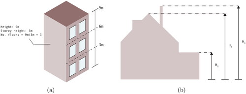
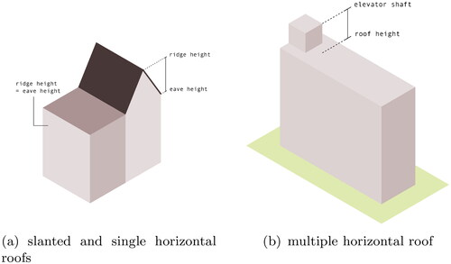
When a 3D model of a building or elevation information (e.g. a point cloud) is available, it is often assumed that deriving the number of floors is a simple geometric task. As shown in Figure 1(a), we can estimate the number of floors by dividing the height of a building with an assumed average storey height (the results are typically rounded to the nearest integer). In a research context, Alahmadi et al. (2013), Nouvel et al. (2014), and Shiravi et al. (2015) all use this geometric method for their applications, and it is the model most often mentioned by practitioners (the Dutch model for flooding uses this method). However, assuming that the number of floors is a simple linear function of the height will only work for simple buildings with flat roofs [which are estimated to account for only 34% of building stock in the Netherlands (Dukai et al. 2019)], and in practice, it may fail for buildings with slanted roofs, those having a floor lobby taller than the floors above, or complex configurations (we give examples in Section 3). As shown in Figure 1(b), the main issue is that it is not clear what the single height of a building should be [we refer to this concept as the height reference (Biljecki et al. 2014)], especially if we have 3D models where the shape of the roofs and extra installations, such as chimneys and antennas are modelled; we elaborate on these concepts in Section 2.

Figure 1. (a) Geometric approach to estimate number of floors from building height. (b) The several height references that can be used to assign one height to a building.

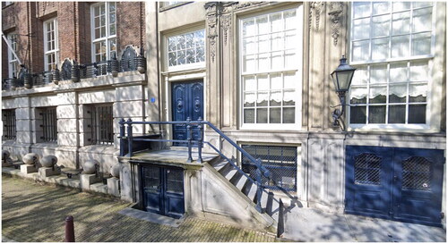
Another alternative to obtain the number of floors is to count the number of windows, in the vertical direction, from street-view imagery (Biljecki and Ito 2021). This method appears to be used by many, e.g. by Shiravi et al. (2015), to manually perform a visual inspection of the results (after having used the geometric method); we used it too during the development of our methodology. However, it should be added that interpreting façade images to unambiguously determine the number of storeys is an intricate task because of the several possible configurations (see for instance Figures 5 and 13), and because of the several occlusions caused by trees and parked cars. Even a human visually inspecting those images could hesitate between two answers. Nonetheless, Iannelli and Dell’Acqua (2017) trained a convolutional neural network (CNN) for residential houses in the USA, and Wu et al. (2021) developed a network to identify where floors are located in an image of a façade (a closely related problem). Those methods are also limited to the availability of street-view images, which are seldom available as open data (open datasets of lidar measurements are nowadays relatively frequent¹).

In this paper we investigate whether other attributes and characteristics related to buildings (footprints, 3D models, cadastral, and census datasets) can help us better predict the number of floors than using just a geometry-based method; we are not aware of any other research project attempting this. We propose and describe in Section 3 several potential indicators, and we present a predictive model that was trained with around 173,000 residential buildings in the Netherlands (for which we have the footprint, the point cloud, and the detailed 3D model). We focus in this paper solely on (mixed-)residential buildings because commercial and other buildings (such as churches, shopping malls, and factories) have often little correlation between the height and the number of floors, and also because our principal application is saving lives in case of flooding: people live in residential buildings. As further described in Section 4, our model achieves an accuracy of 94.5% and a mean absolute error (MAE) of 0.06 for buildings with five floors or less, which is a substantial improvement over the results of the ‘standard’ geometric approach (accuracy of 69.9% and MAE of 0.31). However, above five floors, our model has only a slight improvement on the geometric approach (accuracy of 52.3% and MAE of 0.62, whereas the geometric approach was 47.5% accurate and had an MAE of 0.70). We further elaborate on this in Section 5, but the main culprit is the lack of training data for buildings having more than five floors (Dutch buildings are rarely above 5 floors, see details in Section 3.1). One interesting result of our work is that detailed models with roof shapes (commonly referred to as ‘LoD2’, see Section 2) are not contributing much to having a better model; the simple extrusion of footprints to a single height (Ledoux and Meijers 2011) is sufficient. This fact would allow practitioners to save money on data acquisition and processing if they wanted to obtain the number of floors for their applications.

2. Background and related work

The level-of-detail (LoD) of a 3D model of a building describes its complexity, allowing its degree of resemblance to the real-world situation to be portrayed (Biljecki et al. 2016b). While different categorizations exist, the most widely used standard for specifying the LoD is that of CityGML (Gröger and Plümer 2012, OGC 2012), which has been refined by Biljecki et al. (2016b). LoD1 refers to a block model, which is easily obtained by extruding footprints to a single height. This height is usually obtained by processing the point cloud points inside the footprint (and finding the median after filtering). LoD2 refers to a general model of the building structure including simplified roof shapes. LoD3 models are architecturally detailed and include windows, doors, and chimneys.

Despite the apparent simplicity of the LoD1 block model, there is a high level of ambiguity in its geometric representation (Biljecki et al. 2014). As illustrated in Figure 1(b), the position of the top surface varies significantly depending on the height reference chosen to represent the building’s height. If we are extruding footprints to reconstruct LoD1 models, these height references can be taken into account by using different percentiles of the point cloud’s z-coordinates, those points whose projection on the xy-plane intersects the footprint (Dukai et al. 2019). The 100th percentile would be the highest points (potentially a chimney or an antenna), and the 50th percentile should be around the eave since there will most likely be many points located on the façades of the building. In the context of our work, the height references representing the ridge and eaves are the most important (see Figure 1(b)). The difference between these heights could potentially be used to identify storeys beneath slanted roofs.

The average storey height—used for the geometric approach—is not actually a single, static value, but it varies historically and geographically. For example, in the Netherlands, it is around 2.65 m for buildings built since 2003, but it was around 3 m one hundred years ago (Ministry of the Interior and Kingdom Relations 2012). As a matter of fact, such reasoning can be extended to several other countries, too. For this reason, in our proposed method, we use the construction year of the building as one of the indicators.

3. Datasets and methods

3.1. Datasets

We use three openly available datasets in the Netherlands:

1. BAG: 2D footprints and addresses of all buildings in the Netherlands. Each footprint is associated with several attributes, such as construction year and current use, but the number of floors is currently not included. We used the dataset as of 04–2020 from https://bag.basisregistraties.overheid.nl

2. 3D BAG: 3D models automatically reconstructed (in LoD2) by using a lidar point clouds (Dukai et al. 2021, Peters et al. 2022). We used version 21.03.1 from https://3dbag.nl

3. Census data: we used the 2019 neighbourhood census data from Statistics Netherlands (CBS in Dutch: https://cbs.nl). Since this dataset is only available at a neighbourhood level, buildings from the same statistical neighbourhood received the same value for each feature. A neighbourhood is defined as a homogenous area [in terms of buildings and socio-economical characteristics (CBS 2020)]. As an example, Amsterdam has its 219 km² divided into 481 neighbourhoods, which means that each is about 0.2 km² in size.

We also obtained training data from four municipalities in the Netherlands: Amsterdam,² Rotterdam, The Hague, and Rijssen-Holten (see Figure 2(a)). These municipalities either assigned manually the number of floors or retrieved this information from one of their databases; as shown below the datasets contained noise and errors and we had to (semi-)manually clean them. The first three municipalities correspond to the three largest cities in the Netherlands, while Rijssen-Holten is a more rural municipality located in the west of the country. It was added to provide the algorithms with data that was also representative of less densely populated regions of the country. However, the majority of buildings originate from Rotterdam (Figure 2(b)), meaning that the dataset mainly corresponds to urbanized areas. A comparison of the different training datasets is provided in Table 1.

Figure 2. Overview of training dataset.

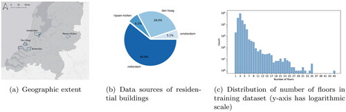
Table 1. Quantitative comparison of the training data by municipalities.

Municipality	# bldgs	Residential bldgs.	Median # floors	Pop. density	# clean bldgs
Amsterdam	22,328	64%	4	5.21k/km^2	8757
Rotterdam	206,809	56%	3	2.96k/km^2	105,245
The Hague	53,730	99%	3	6.52k/km^2	48,450
Rijssen-Holten	11,879	97%	3	0.41k/km^2	10,700
Total	294,746	67%	3		173,152

Since each municipality has a different approach towards storing the number of floors, we cleaned the input datasets to remove any obvious errors (e.g. where the number of floors was zero or a negative value) and to somehow standardize the data. In addition, we filtered the data to keep only the residential buildings and those that are semi-residential (most often having shop on the ground floor and apartments above, see Figure 5(a) for one example); the filtering was performed on an attribute of the BAG.

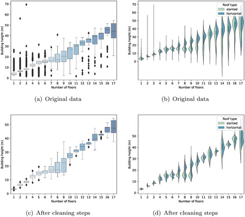
We further cleaned the training data because it contained several (gross) errors, this was carried out using a combination of (semi-)automatic and manual steps. As can be seen in Table 1, in total 59% of the input data on the number of floors remained after cleaning. The cleaning steps mainly focused on removing obvious errors and outliers from the data. To speed up the data cleaning process, the strong correlation between building height and the number of floors was utilized. As shown in Figure 3, we used box plots to filter erroneous labels, e.g. we removed all values above the 75th percentile and under the 25th percentile. We also used violin plots show the probability density of the data distribution (Hintze and Nelson 1998), these plots were used to show the distribution for slanted and horizontal roofs separately, allowing the influence of roof type to be analysed. Cases where the number of floors was missing (i.e. zero or NULL), larger than 48 or <0 were removed, as well as any duplicate buildings. Also, since there was an insufficient number of buildings to provide reliable trends above 17 floors, the semi-automatic cleaning process was not performed for buildings with more than 17 floors. Instead, these buildings were cleaned through manual inspection using Google Street View.

Figure 3. Semi-automatic data cleaning steps.

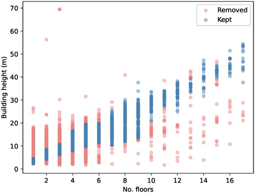
We chose to aggressively remove wrong labels (thus removing about 40% of the data that were available) to ensure that the training data was—as much as possible—free of errors, although this came at the cost of removing good labels (Figure 4).

Figure 4. Scatter plot of buildings kept and removed by the semi-automatic cleaning steps.

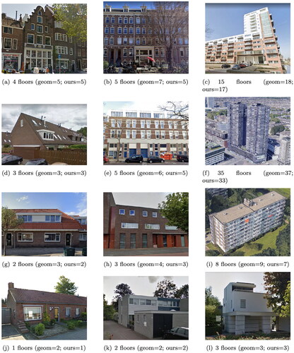
After cleaning, the training dataset consists of 173,152 buildings, ranging from 1 to 45 floors. These buildings cover a variety of architectural styles, construction periods, and building types. A number of examples from each municipality are provided in Figure 5. These buildings are used as case studies during the analysis in order to gain a more concrete understanding of model performance. Some examples were selected to represent particularly challenging aspects of the prediction problem. For instance, buildings with varying storey heights, elevator shafts, or multiple storeys beneath slanted roofs. The example shown in Figure 5(b) was selected because the building in the centre has one floor less than its neighbours due to a double-height café on the ground floor. The geometric approach would be unable to distinguish these cases.

Figure 5. Examples of buildings in the training dataset. The results obtained with the standard geometric approach (geom) and our results with machine learning (see Section 4) are between parentheses. Source: Google Street View (2022).

As shown in Figure 2(c), the training dataset is quite heavily skewed towards buildings with lower numbers of storeys (around 90% of the available training data consists of buildings with 5 floors or less). Data imbalance is problematic because most machine learning algorithms aim to minimize the overall error rate (Chen and Breiman 2004). In order to take data imbalance into account, we report on our results in Section 4 low (≤5) and high (>5) storey buildings separately. This prevents the prediction errors for high storey buildings from being masked by the results for low storey buildings. Furthermore, a stratified approach was used to create the train-test split. This stratification was based on building height since this is known to be highly correlated to the number of floors (Biljecki et al. 2017).

3.2. Predictors for the number of floors

We looked at different studies where the heights of buildings are predicted from different predictors, and we compiled the 19 predictors shown in Table 2. Those features are subdivided into 4 classes: (1) cadastral; (2) 2D geometric (based footprints); (3) 3D geometry (based on the 3D model); (4) and census-based features. The relevance of the features is explained in the table. Notice that since the 3D geometry-based predictors are computed for both the LoD1 and LoD2 models, we obtain a total of 25 potential predictors (which we call features).

Table 2. Features used are classified into four classes: cadastral, 2D geometric, 3D geometric, and census.

	Feature	Details and relevance
1	Construction year	Construction period is often related to storey height. For instance, after 2003, the Dutch building code increased the required storey height of new buildings from 2.4 to 2.6 m (Ministry of the Interior and Kingdom Relations 2012). This means that construction year could be used to distinguish buildings with the same number of floors but different heights.
2	Building function	A distinction is made between residential and mixed-residential, as mixed-residential buildings have been found to exhibit different properties than purely residential buildings (Biljecki et al. 2017).
3	Net internal area	Previous research has found that taller buildings (with more storeys) generally have a higher net internal area (Biljecki et al. 2017).
4	Number of units	Similar to the net internal area, buildings with more storeys generally contain more building units (e.g. apartment blocks).
5	Building type	4 possible values: detached, semi-detached, terraced and apartment blocks. Apartment blocks generally have a higher number of floors than (semi-) detached and terraced buildings
6	Area	Dividing the net internal area by the footprint area can provide an indication of the number of floors.
7	Perimeter	In combination with area, perimeter can provide information about the footprint shape, such as its compactness and complexity (Lánský 2020).
8	No. vertices	A higher number of footprint vertices could indicate a more complex shape (Lánský 2020). Computed after simplification by Douglas-Peucker.
9	No. neighbours	The number of neighbouring building centroids within a 100 m radius of the footprint centroid. Buildings with many storeys are generally surrounded by more open space (Biljecki et al. 2017). Buildings in rural areas also generally have fewer neighbours (Lánský 2020).
10	No. adjacent buildings	The number of buildings within a 0.1 m buffer of each footprint. Lower storey buildings in urban areas generally have more immediate neighbours.
11	Building height	Computed for the minimum, maximum, 50th and 70th roof height percentiles (available as attributes of the 3DBAG). Building height is strongly related to number of floors, especially for residential buildings (Biljecki et al. 2017).
12	Roof shape	An attribute provided for each building in the 3DBAG. In combination with building height, roof shape could provide information about the likelihood that storeys are present beneath slanted roofs.
13	Ridge-eave heights	The difference between the height of the ridge and eaves of the roof. Similar to roof shape, this could provide some indication of whether storeys might be present beneath slanted roofs (Figure 6).
14	Roof surface area	Computed for both LoD1 and LoD2 to describe building geometry.
15	Wall surface area	Computed for both LoD1 and LoD2 to describe building geometry.
16	Building volume	Computed for both LoD1 and LoD2. A larger volume is somewhat linked to a larger number of floors.
17	Population per km^2	Areas with a higher population density generally have more high storey buildings to accommodate all residents.
18	Percent multi-household	Multi-household buildings, such as apartment blocks, generally have more storeys than single family homes.
19	Average # of cafés <1 km	The average number of cafés shows a strong link to area morphology and could be used to distinguish central business districts from rural and suburban areas. Other amenities were also considered but the average number of cafés showed the clearest relationship to area morphology. The CBS dataset we use contains the number of amenities within 1 km, but other sources, such as OpenStreetMap could easily be used.

Most predictors are attributes in the datasets we use or result from simple GIS operations. Only three require more details:

#13 ridge-eave heights: this was computed from the LoD2 model. For slanted roofs, ridge height was computed as the 90th percentile of the roof surface z-coordinates while eave height was computed as the 75th percentile (Figure 6(a)). For buildings with completely horizontal roofs, ridge height was computed as the 90th percentile of the roof surface z-coordinates, minus ground height. We also extended this to buildings with multiple horizontal roof surfaces, to potentially allow buildings with elevator shafts and other roof installations to be distinguished (Figure 6(b)). These structures increase the measured height of a building, but should not contribute to the floor count. An attempt was made to define ridge and eave height in such a way that they could be used to distinguish buildings with elevator shafts. A larger difference between these percentiles could indicate that elevator shafts are present. However, the disadvantage of this approach is that the 75th percentile could also correspond to lower roof sections, such as balconies or porches.

Figure 6. Ridge vs. eave height based on roof type.

#14/15 roof + wall surface areas: computed from both the LoD1 and LoD2 models.

#16 building volume: in our LoD2 dataset, more 95% of the buildings are geometrically and topologically valid (Ledoux 2018), but it is in practice often significantly lower (Biljecki et al. 2016a). If the solid contains errors (gaps, self-intersections, etc.) then it is not possible to compute its volume by using its geometry. For those buildings, we implemented our own version of the voxel-filling algorithm of Steuer et al. (2015), which gives in most cases a reliable approximation.

3.3. Predictions models

Is inferring the number of floors a regression or a classification problem? On the one hand, floor count is generally an integer value, which could be predicted as discrete classes by a classification algorithm or obtained after rounding the predictions of a regression algorithm. However, classification would require the training data to include examples of all possible floor counts that exist in reality. In practice, it would be difficult to find this data, meaning that the model would be unable to predict the number of floors of the missing classes. In contrast, the predictions of a regression model are not limited to the training data examples, allowing predictions to be made also for unseen cases. The model takes into account the ordinal nature of the number of floors and remains applicable to new buildings with higher floor counts. A further advantage of regression is that floor count is predicted as a decimal value, allowing buildings with ‘half floors’ to be taken into account. This is required for certain applications, such as energy demand estimation. Therefore, we consider the number of floors as a regression problem.

Three different predictive models were trained: Random Forest (RF), Gradient Boosting (GB), and linear Support Vector Regression (SVR). The training process was performed using an iterative approach and some data preparation steps, such as data cleaning, were repeated throughout the process (as explained in Section 3.1). We used 80% of the 173,152 cleaned buildings for the training, and the other 20% was kept for testing. A stratified approach was used to create the train-test split, this stratification was based on building height since this is known to be highly correlated to the number of floors.

Each model was first trained on all available features and then trained with three subsets of the features. As explained in Section 4.1, we used for each two filter methods and one embedded method (using the model weight for the SVR). The hyperparameters of the best model of each algorithm were tuned, see Section 4.2 for details. Based on these, the SVR turned out to perform poorly. Both RF and GB performed similarly, GB having a slightly better prediction accuracy. In the following, we focus on the GB model, and the final results are obtained by tuning its hyperparameters (see Section 4.2).

3.4. Data handling and software

The methodology was implemented entirely in Python using:

1. scikit-learn library (Pedregosa et al. 2011) for the prediction models;

2. PostGIS (Strobl 2008) to store all input datasets;

3. the 2D geometric features were extracted with PostGIS functions;

4. the 3D geometric features were implemented by ourselves

Our code is publicly available at: https://github.com/ellieroy/no-floors-inference-NL.

4. Results and evaluations

We trained four Gradient Boosting (GB) models, one with all the 25 features in Table 2, and three with different subsets of 10 features (obtained with statistical analysis, see Section 4.1).

To evaluate the performance of these models, the MAE (mean absolute error), the RMSE (root mean square error), maximum error, and accuracy were computed on the predictions obtained for the test dataset (20% of the cleaned buildings). We report these metrics separately for buildings with 5 floors or fewer, and for those with more than 5 floors, to distinguish the errors caused by high-rise buildings with low data availability. Buildings with 5 or fewer floors represent around 90% of the training dataset.

We then tuned the hyperparameters of the best model (GB-2) (this is further detailed in Section 4.2), and this allowed us to greatly improve the model. Its final accuracy is 94.5% for buildings containing 5 floors or less, and 52.3% for taller ones. After tuning the hyperparameters, the MAE was almost halved and the maximum error for buildings taller than 5 floors was reduced by one floor (but for 5 floors and less it increased by one).

You can see the results for the standard geometric approach (as explained in the Introduction), it is the row ‘Geom.’ in Table 3. Building height was based on the 70th percentile of the lidar inside the footprint (all feature selection methods have the 70th percentile as the best predictor, see Section 4.1), and an assumed storey height of 2.65 m was used [this value is derived from the Dutch building code (Ministry of the Interior and Kingdom Relations 2012)]. As is the case for our model, the results were rounded to the nearest integer rather than rounded down. This reduces the likelihood of overestimation, which is useful for one of the main applications in Netherlands, flooding assessment since overestimation could potentially cause the presence of dry floors to be incorrectly identified.

Table 3. Model evaluation results, for ≤5 and >5 floors.

	Hyper	MAE		RMSE		Max error		Accuracy (%)
		≤5	>5	≤5	>5	≤5	>5	≤5	>5
GB-all	No	0.11	0.98	0.33	1.29	2	4	89.6	25.6
GB-1	No	0.11	1.04	0.33	1.36	2	5	89.4	24.1
GB-2	No	0.11	0.98	0.33	1.31	2	5	89.6	27.0
GB-3	No	0.12	1.02	0.25	1.33	2	4	88.4	23.7
GB-2	Yes	0.06	0.62	0.24	1.00	3	4	94.5	52.3
Geom.	N/a	0.31	0.70	0.57	1.09	2	5	69.9	47.5

These results show that our model performs better according to all four error metrics, apart from the maximum error for buildings with ≤5 floors. For buildings below 6 floors, the best model has a much lower MAE and is ∼25% more accurate than the geometric approach. In addition, for buildings above 5 floors, the performance difference is less notable.

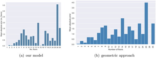
It is interesting to note that, similar to machine learning, the geometric approach performs worse for higher storey buildings (Figure 7). This suggests that the number of floors of these buildings is inherently more difficult to predict. This could be due to building characteristics, such as the presence of elevator shafts or double storey ground floor lobbies. The input data (quality and completeness) could also play a role. As a result, machine learning may require more training instances of high storey buildings to reach a similar level of performance to lower storey buildings.

Figure 7. Mean absolute error per number of floors.

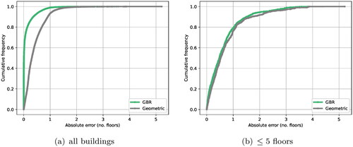
The cumulative error distributions of our final model and that of the geometric approach are shown in Figure 8. These plots show the fraction of buildings with an error less than or equal to a certain number of floors. If all buildings are considered (Figure 8(a)), the number of floors is predicted within 1 floor of the true value in ∼99% of cases for our model, and in only 90% for the geometric approach. If buildings above 5 floors are considered separately (Figure 8(b)), the cumulative error distributions are almost identical. This shows that even the best predictive model does not provide a substantial improvement on the current estimate.

Figure 8. Cumulative errors of the best predictive model compared to geometric approach.

Figure 8 shows the results obtained with the geometric approach and our model. This analysis was conducted to ensure that the performance differences were not always caused by incorrectly labelled buildings. The results show that our model provides a better estimate of the number of floors for buildings with larger than average storey heights. For example, the five-storey building in Figure 5(e), and three-storey building in Figure 5(h) have slightly higher storey height than average. These examples were predicted correctly by our model, whereas they were overestimated by the geometric approach. In addition, our machine learning model provides a more accurate estimate for the five-storey building in Figure 5(b) with a café on the ground floor. The neighbouring buildings are purely residential and have 6 floors, whereas the building with the café has only 5 floors due to the double-height ground floor. The geometric approach could not distinguish this case and provided an overestimate of 2 floors. Machine learning was also able to distinguish buildings with and without storeys beneath slanted roofs. For instance, the number of floors of the single-storey building with a slanted roof in Rijssen-Holten was predicted correctly. This example was overestimated by the geometric approach because the slanted roof increased the measured height of the building. The slanted roof of the 2-storey building in Den Haag also caused the geometric approach to overestimate the number of floors. None of the approaches were able to correctly determine the floor count of the four-storey building in Figure 5(a). The number of floors was overestimated by 1 floor in both cases. This is most likely due to the differences in storey height throughout the building. Furthermore, both approaches performed worst for the examples of high storey apartment blocks. Our model generally underestimated the number of floors of these buildings, whereas the geometric approach provided an overestimate.

4.1. Feature selection

We performed feature selection to determine which features have the best prediction power and to eliminate any redundant or irrelevant features. This allows us to reduce the number of input variables that the model has to fit, which lowers the computational cost of training. Secondly, only the most relevant features are used and less useful features are removed, reducing noise in the training data. Furthermore, the performance of the model may be improved since the algorithm does not focus on fitting the model to irrelevant features, which could lead to an overfit on the training data.

To rank and select the features according to their predictive power, we have used and compared different methods.

First, we have used two filter methods: (1) Pearson correlation coefficient and (2) the Mutual Information (MI) methods. The benefit of this filter methods is that it is computationally light and independent of the machine learning algorithm used (Chandrashekar and Sahin 2014). This means that the likelihood of overfitting is reduced, as the selection is not tuned for a specific learning algorithm (Guyon and Elisseeff 2003). The top ten features based on MI and Pearson’s correlation coefficient are shown in Table 4. The two filter methods provide very similar results, the top five features are the same in both cases and the results differ by only one feature overall. As expected, building height has the strongest level of correlation, with 70th percentile height ranking highest for both methods. Two other 3D geometric features, roof area, and volume, are also found to be related to the number of floors. Please observe that the correlation is approximately the same, irrespective of the LoD of the model.

Table 4. Top ten features selected by different methods.

	Mutual information		Pearson correlation		Embedded GB
	Feature	Value	Feature	Value	Feature	Value
1	Height (70th)	1.00	Height (70th)	1.00	Height (70th)	0.883
2	Height (max)	0.89	Height (max)	0.79	Height (max)	0.071
3	Height (50th)	0.85	Height (50th)	0.58	Net internal area	0.020
4	Roof area (LoD1)	0.63	Roof area (LoD1)	0.11	No. units	0.005
5	Roof area (LoD2)	0.60	Roof area (LoD2)	0.11	Height (50th)	0.004
6	Net internal area	0.59	No. units	0.05	Construction year	0.004
7	Volume (LoD1)	0.51	Volume (LoD1)	0.04	Roof area (LoD2)	0.003
8	Volume (LoD2)	0.50	Volume (LoD2)	0.04	Avg. no. cafés in 1 km	0.002
9	Population density	0.47	Net internal area	0.03	% multi-household	0.001
10	% multi-household	0.34	% multi-household	0.03	Ridge-eave height	0.001

Second, we have used embedded methods, which are integrated as part of the training process, meaning they are dependent on the machine learning algorithm used. The importance of each feature is derived based on its contribution to the predictive model. The interaction between features is taken into account, enabling a better understanding of the training dataset to be obtained. A common example of an embedded method is the impurity-based feature importance built into tree-based models (Lal et al. 2006). The top 10 features for the Gradient Boosting (BG) are shown in Table 4. As is the case for the filter method, the 70th percentile building height is the most important feature. However, fewer 3D geometric features are selected. Furthermore, unlike the filter-based method, the LoD2 features rank higher than their LoD1 equivalents, which are not included in the feature subsets. It is also interesting to note that 70th percentile building height has a much higher importance than all other features combined. However, since the importance scores are based on the training set, the other features could still be useful for predicting the number of floors of unseen cases.

Overall, the results of the filter and embedded methods are quite varied, highlighting the difficulty to select the best subset. However, several features were not included in any of the subsets, suggesting they are not relevant to the prediction problem. These features were: wall surface area, building function, and all 2D geometric features, aside from the number of neighbours.

A drawback of filter and embedded methods is that the selected subsets include many similar features. This is because these are not independent, and may have a high level of correlation between them. We calculated the level of correlation between the input features with the variance of an independent variable method (VIF), which is shown in Table 5 for features selected by the MI and the embedded-GB methods. The VIF describes the extent to which the variance of an independent variable is increased by its correlation to other variables; a value of 1 indicates the absence of collinearity and, as a general rule of thumb, values above 5 or 10 indicate high collinearity (James et al. 2021). The VIF scores show that there is a high level of multicollinearity present in the selected feature subsets, particularly for the filter-based subset. Seven of the features selected using the filter-based method have a VIF score higher than 5. The subset based on GB feature importance performs slightly better, as the number of features with a VIF score higher than 5 is reduced to five.

Table 5. Variance inflation factor (VIF) of two feature subsets.

	Mutual information		Embedded GB
	Feature	Value	Feature	Value
1	Height (70th)	51.8	Height (70th)	44.9
2	Roof area (LoD1)	38.6	Height (max)	27.6
3	Volume (LoD1)	26.5	Height (50th)	18.2
4	Height (50th)	23.0	Roof area (LoD2)	9.2
5	Roof area (LoD2)	21.6	No. units	5.1
6	Height (max)	20.0	Net internal area	2.4
7	Volume (LoD2)	17.0	% multi-household	1.9
8	Net internal area	4.7	Ridge-eave height	1.8
9	% multi-household	2.0	Avg. no. cafés in 1 km	1.6
10	Population density	1.9	Construction year	1.4

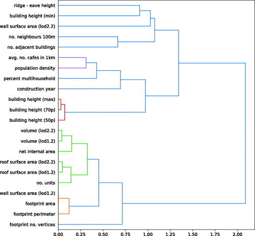
To reduce the groups of correlated features, we applied hierarchical clustering, a process that enables closely related variables to be grouped together based on a similarity measure (Rokach 2010). We used Ward’s linkage, which computes the ‘distance’ between two clusters as the increase in the error sum of squares after merging two clusters together. The resulting clusters are visualized by the dendrogram shown in Figure 9. A threshold distance of 0.4 was used to assign features to the same cluster. This value was chosen to group together as many similar features as possible. The groups shown in red, green, orange, and purple represent different clusters, while the features linked in blue were not assigned to a cluster.

Figure 9. Hierarchical clustering between input features based on the Pearson correlation coefficient.

To select a feature subset with reduced multicollinearity, a filter-based approach was first performed on each cluster. The feature with the highest MI score was selected per cluster. Then, the features with the ten highest MI scores were selected from the best feature per cluster and the remaining unclustered features. The results are shown in Table 6, alongside the MI scores. It is noticeable that the MI score of some features is quite low. However, a number of these features were also considered important by the embedded method. Features with low individual relevance can still be useful when combined with other features (Guyon and Elisseeff 2003). For comparison, the VIF scores are also shown. All scores are lower than 10 and only one feature has a score slightly higher than 5, showing that multicollinearity was successfully reduced.

Table 6. Feature subset with reduced multicollinearity.

	Feature	MI score	VIF score
1	Building height (70th)	1.00	3.28
2	Roof area (LoD2)	0.60	6.63
3	Population density	0.47	2.16
4	% multi-household	0.35	2.30
5	Construction year	0.24	1.31
6	Footprint perimeter	0.18	4.34
7	Building height (min)	0.14	1.09
8	Ridge-eave height	0.12	1.17
9	No. adjacent buildings	0.05	1.29
10	No. neighbours in 100 m	0.04	1.42

4.2. Hyperparameters tuning

Because hyperparameters control the learning process, tuning them can help to improve a model’s generalization performance. This means that the algorithm will be able to generate a model that provides a good fit to the training data, but will also perform well on other unseen data. We can see in Figure 3 that this was indeed the case, especially for the buildings with more than 5 floors.

There are six hyperparameters to tune for Gradient Boosting: (1) maximum depth of each tree in the ensemble; (2) minimum number of samples of leaf nodes; (3) minimum number of samples of internal nodes; (4) maximum number of features; (5) number of trees in the ensemble; (6) learning rate. To tune our model, as shown in Figure 10, a grid of possible values for each hyperparameter was created. A randomized search was performed over 75 different combinations of these values. This means that our model was trained 75 times on different combinations of the hyperparameter values provided. As a result, not all possible combinations were tested. However, this approach was preferred over an exhaustive search since this would have a much higher computational cost.

Figure 10. Visualization of train-test split and cross-validation. Adapted from Scikit-learn (2007–2021).

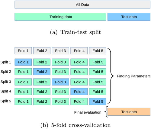
To determine appropriate parameter values to test, validation curves for each hyperparameter were plotted. Figure 11 shows three of them, but this was done for all six. To obtain such a plot, each hyperparameter was altered in isolation and 5-fold cross-validation was used to evaluate model performance. Since the dependence between hyperparameters is not considered, these plots are not fully representative of the impact on model performance. However, they are still useful to gain an initial understanding of which values to test. The impact of each hyperparameter on the model performance was assessed using the RMSE because of its higher sensitivity to larger errors.

Figure 11. Validation curves for three Gradient Boosting hyperparameters.

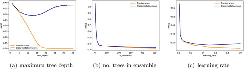
Figure 11(a) shows that increasing the tree depth initially led to a reduction in RMSE for both the training and cross-validation sets. However, beyond a certain depth, the cross-validation error no longer improved and even began to increase. At the same time, the training error continued to decrease until a plateau. This shows that increasing the maximum tree depth caused the model to overfit the training set and prevented it from generalizing to the test set.

Increasing the number of trees generally leads to better model performance, however using many trees also slows down the training process. Figure 11(b) shows that the RMSE was reduced by increasing the number of trees. The decrease in RMSE was initially very high, since using only a few trees causes the algorithm to underfit the training data. Beyond a certain point, the decrease was more gradual, showing that using more trees does not substantially improve model performance.

The contribution of each tree is determined by the learning rate parameter. A lower learning rate means that more trees are required to fit the data, but generally results in better model generalization (Géron 2019). Figure 11 shows that increasing the learning rate initially led to a reduction in RMSE. However, when the learning rate became higher, the gap between the two curves increased. This shows that the model started to overfit the training data and did not generalize well to the validation set.

4.3. Impact of rounding on results

Figure 12(a) shows the distribution of the fractional part of all predictions (before rounding to the closest integer). It is interesting to observe that most predictions have a fractional part of either below 0.1 or above 0.9. This suggests that our rounding strategy did not have a large impact on the results, as the majority of predictions were already very close to an integer value.

Figure 12. Analysis of fractional part of predictions.

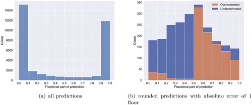
It is also interesting to determine how often the fractional part caused the model to over- or under-estimate the target value after rounding. This was achieved by analysing the fractional part of predictions that had an absolute error of 1 floor after rounding (Figure 12(b)). The results show that increasingly more predictions were over- or under-estimated the closer the fractional part got to the halfway point between two integers, which makes sense as this is the most ambiguous case. The distribution is quite balanced, meaning that rounding caused a similar number of over- and under-estimations.

Furthermore, an over-estimation of 1 floor after rounding was mainly caused by fractional parts of above 0.5. Relatively few cases were overestimated by 1 floor because the fractional part was <0.5. This occurs when the predicted value is 1–1.5 floors larger than the target (e.g. a prediction of 3.1 for a target value of 2). Conversely, an underestimation of 1 floor after rounding was mainly caused by fractional parts below 0.5. Relatively few cases were underestimated by 1 floor because the predicted value was 1 to 1.5 floors smaller than the target (e.g. a prediction of 1.8 for a target value of 3).

4.4. Impact of data availability

The impact of data availability was assessed by training our predictive model (after tuning the hyperparameters) on different categories of features. This provides us with an indication of our model performances when certain datasets are unavailable, for instance, LoD2 models might not be available in other countries. This also provides us with another perspective on how different features contribute to the model.

The results are shown in Table 7.

Table 7. Impact of different feature subsets on model performance.

	Features					Model performance
	Cadastral	Geometric			Census	MAE		Accuracy (%)
		2D	LOD1	LOD2		≤5	>5	≤5	>5
1	×	×	×	×	×	0.05	0.64	94.8	51.7
2	×					0.19	1.35	82.5	25.3
3		×				0.39	2.23	65.2	5.8
4			×			0.10	0.89	90.1	32.5
5				×		0.10	0.87	90.5	34.8
6					×	0.41	2.55	61.7	3.6

The first model was based on all features to establish a baseline scenario in which all datasets are available. The models with the most comparable performance to this baseline were those based on the LoD1 and LoD2 features. The model based on LoD2 performed slightly better than LoD1. However, overall, there was very little difference in performance, showing that a higher level of detail is not necessarily required. A similar quality of predictions can be obtained based on LoD1.

The model based on cadastral features had the next best performance. For buildings below 5 floors, the MAE was almost double that obtained using the 3D geometric features. In addition, the MAE above 5 floors was almost half a floor higher. On the other hand, the accuracy was only reduced by around 8% and was more than 80% for buildings with <5 floors. This shows that the 3D geometric features are more useful for reducing the prediction error, but a reasonably good level of accuracy can still be achieved with just cadastral features.

The worst performing models were those based on the census and 2D geometric features. These models provided an accuracy of around 60–65% below 5 floors, but only 5% or less for higher storey buildings. For buildings below 5 floors, the MAE of these models was almost the same, suggesting that these feature categories contribute a similar amount to model performance. However, the accuracy of the model based on census features was lower. This model also made larger prediction errors for buildings above 5 floors, showing that the 2D geometric features are slightly more useful. This makes sense as the 2D geometric features were extracted per footprint, whereas the census features were only available at a neighbourhood level.

An accuracy of around 60% is still quite high, which is particularly surprising for the model based on neighbourhood census data. This can be explained because a high level of accuracy (55.5%) can still be achieved if the mean number of floors is predicted for all buildings. However, the subset based on census features still achieves a 5% higher accuracy than the model based on the mean. This shows that the additional context that these features provide about the building’s surrounding environment helps to improve model performance.

5. Conclusions

We have shown that the standard geometric method, widely used by practitioners and researchers, to estimate the number of floors of a building (i.e. dividing its height by an assumed storey height, and rounding) has serious limits, especially for buildings with slanted roofs, or when elevators shafts are present, or when a building has a shop and/or restaurant on the ground floor. For a dataset in the Netherlands, this method yields an accuracy of 69.9% for residential buildings with 5 floors or less, and 47.5% for the others.

The machine learning model we have designed, using the Gradient Boosting algorithm, uses other attributes and characteristics of residential buildings to help better infer the number of floors. It improves significantly on the geometric method: 94.5% for buildings with 5 floors or less, and 52.3% for the others. We have defined and analysed 25 potential features (from cadastral attributes, building geometry at different LoDs, and neighbourhood census data), and unsurprisingly our results show that building height, particularly 70th percentile height, is most related to the number of floors. Other 3D geometric features are also found to be quite closely related to the number of floors, specifically roof area, and volume. Furthermore, models based on a combination of different features performed better than models based on single categories of features. It should be stressed that a higher level of detail did not improve significantly the results, i.e. reconstructing the LoD2 of a building, a complex and costly operation, is not always necessary. If only footprints, some cadastral attributes, and an elevation point cloud are available, then it is possible to obtain reliable floor number predictions.

The results we obtained for residential buildings containing more than 5 floors do not represent a significant improvement over the geometric approach, this is because the training dataset was not representative of these buildings: around 90% of the available training data consisted of buildings with 5 floors or less. As a result, it was more difficult for machine learning to infer patterns for higher storey buildings. This shows that better predictions can only be obtained if sufficient training instances are available (which is not the case in the Netherlands).

One limitation of our approach is that we did not have training data for so-called ‘half-floors’ (an example is shown in Figure 13), which are quite common in the old part of Amsterdam for instance. This prevented us from training our model for such cases. Furthermore, the training data we obtained was in many cases not reliable, and a rather complex and time-consuming cleaning process needed to be done, causing a large amount of data to be removed. Also, model performance was assessed in terms of absolute measures of performance. However, it would have been interesting to consider the relative error distribution, since an error of 1 floor is more significant for a one-storey building than a high storey apartment block. Finally, while the influence of different height percentiles on the results of the geometric approach was not considered, our data suggest it is the most accurate. We have indeed tested four different heights as features (0-, 50, 70-, 100-percentile), and for all the feature selection methods we used (see Section 4.1), the 70-percentile was the feature with the best prediction.

Figure 13. Example of a ‘half-floor’ for a building in Amsterdam. Notice how the adjacent building does not have this half-floor. Source: Google Street View (2022).

It should be noticed that our model can be used directly to predict the number floors in the Netherlands and potentially in neighbouring European countries that have similar building regulations and characteristics. However, for countries in the Americas or in Asia, where typical buildings can be significantly different, training data would need to be used and a specific model trained. This model would potentially have different predictors than the ones we used. Our model can however also be used as a mechanism to control the data that municipalities have. As mentioned in Section 3.1, the data we obtained from municipalities were far from being perfect (often outliers and gross errors were present). Based on our model, it would now be relatively easy for a municipality to identify which buildings have errors, and thus to only control manually those.

For future work, we would like to obtain more training data, especially for buildings above 5 floors. We will need to look at other countries and potentially use OSM datasets, however at the cost of further data quality assessment and cleaning steps. We would also like to investigate whether different features would be needed for tall buildings and whether the accuracy of around 52% could be improved.

Acknowledgements

We would like to thank the municipalities of Amsterdam, The Hague, Rotterdam, and Rijssen-Holten for providing training data for this project.

Disclosure statement

No potential conflict of interest was reported by the author(s).

Data and codes availability statement

The training data are from four municipalities in the Netherlands, only Amsterdam is openly available (accessible via their FTP server: ftp.data.amsterdam.nl). The other three asked to not distribute further the data.

Other datasets used:

1. BAG: open dataset at https://bag.basisregistraties.overheid.nl

2. 3D BAG: open dataset at https://3dbag.nl

3. Census data: open dataset at https://cbs.nl

The code used is available there: https://github.com/ellieroy/no-floors-inference-NL

Additional information

Notes on contributors

Ellie Roy

Ellie Roy is a recent graduate from Delft University of Technology, where she obtained both an MSc in Geomatics (cum laude) and BSc in Applied Earth Sciences. Her master’s thesis focused on the application of machine learning to infer the number of floors of building footprints in the Netherlands.

Maarten Pronk

Maarten Pronk is a researcher at Deltares and an external PhD candidate at the Delft University of Technology. He holds an MSc in Geomatics and a BSc in Architecture, both from the Delft University of Technology (NL). His research concerns elevation modelling, especially in lowlands prone to coastal flooding. He aims to combine his interests in remote sensing and software engineering for societal impact. He promotes open and reproducible research and is the author of several open-source software packages for handling geospatial data, written in the Julia programming language. His work often involves handling trillions of elevation measurements, requiring a careful selection and design of both spatial storage formats and processing algorithms. Currently, he works on applying data from ICESat-2, a LiDAR satellite, on global elevation models.

Giorgio Agugiaro

Giorgio Agugiaro is currently an assistant professor in the 3D Geoinformation research group at TU Delft. In 2002 he received his MSc degree in environmental engineering from the University of Padova (Italy) and in 2009 a PhD in Geomatics from the University of Padova and TU Berlin. Before moving to Delft in 2018, he worked as a researcher at Fondazione Bruno Kessler (Trento, Italy), at TU Munich, and at the Austrian Institute of Technology (Vienna, Austria). His main research interests are in the field of Geographical Information Systems and spatial data integration, with particular focus on semantic 3D city modelling and their energy-related topics. Having a semantic 3D virtual city model as background, the idea is to foster software integration to allow complex urban system simulation and close (or reduce) the gap between geo-information and simulation.

Hugo Ledoux

Hugo Ledoux is an associate professor in 3D geoinformation at the Delft University of Technology in the Netherlands. He holds a PhD in computer science from the University of South Wales (UK) and a BSc in geomatics engineering from the Université Laval (Québec City, Canada).

Notes

1 See for instance https://opentopography.org.

2 The dataset from Amsterdam is the only openly available dataset (accessible via their FTP-server: ftp.data.amsterdam.nl).

References

- Agugiaro, G., 2016. First steps towards an integrated CityGML-based 3D model of Vienna. ISPRS Annals of Photogrammetry, Remote Sensing and Spatial Information Sciences, III-4, 139–146.
- Agugiaro, G., 2016. Energy planning tools and CityGML-based 3D virtual city models. Experiences from Trento (Italy). Applied Geomatics, 8 (1), 41–56.
- Alahmadi, M., Atkinson, P., and Martin, D., 2013. Estimating the spatial distribution of the population of Riyadh, Saudi Arabia using remotely sensed built land cover and height data. Computers, Environment and Urban Systems, 41, 167–176.
- Biljecki, F., 2020. Exploration of open data in Southeast Asia to generate 3D building models. ISPRS Annals of the Photogrammetry, Remote Sensing and Spatial Information Sciences, VI-4/W1-2020, 37–44.
- Biljecki, F. and Ito, K., 2021. Street view imagery in urban analytics and GIS: A review. Landscape and Urban Planning, 215, 104217.
- Biljecki, F., et al., 2016a. The most common geometric and semantic errors in CityGML datasets. ISPRS Annals of the Photogrammetry, Remote Sensing and Spatial Information Sciences, IV-2/W1, 13–22.
- Biljecki, F., Ledoux, H., and Stoter, J., 2014. Height references of CityGML LOD1 buildings and their influence on applications, 11.
- Biljecki, F., Ledoux, H., and Stoter, J., 2016b. An improved LOD specification for 3D building models. Computers, Environment and Urban Systems, 59, 25–37.
- Biljecki, F., Ledoux, H., and Stoter, J., 2017. Generating 3D city models without elevation data. Computers, Environment and Urban Systems, 64, 1–18.
- Boeters, R., et al., 2015. Automatically enhancing CityGML LOD2 models with a corresponding indoor geometry. International Journal of Geographical Information Science, 29 (12), 2248–2268.
- CBS, 2020. Kerncijfers wijken en buurten 2020. Statistics Netherlands. https://www.cbs.nl/nl-nl/maatwerk/2020/29/kerncijfers-wijken-en-buurten-2020.
- Chandrashekar, G. and Sahin, F., 2014. A survey on feature selection methods. Computers & Electrical Engineering, 40 (1), 16–28.
- Chen, C. and Breiman, L., 2004. Using random forest to learn imbalanced data. Berkeley, CA: University of California, Berkeley.
- Dukai, B., et al., 2021. Quality assessment of a nationwide data set containing automatically reconstructed 3D building models. The International Archives of the Photogrammetry, Remote Sensing and Spatial Information Sciences, XLVI-4/W4-2021, 17–24.
- Dukai, B., Ledoux, H., and Stoter, J., 2019. A multi-height LoD1 model of all buildings in the Netherlands. ISPRS Annals of the Photogrammetry, Remote Sensing and Spatial Information Sciences, IV-4/W8, 51–57.
- Fan, H., et al., 2014. Quality assessment for building footprints data on OpenStreetMap. International Journal of Geographical Information Science, 28 (4), 700–719.
- Géron, A., 2019. Hands-on machine learning with scikit-learn, keras, and tensorflow. Sebastopol, CA: O’Reilly.
- Gröger, G. and Plümer, L., 2012. CityGML – interoperable semantic 3D city models. ISPRS Journal of Photogrammetry and Remote Sensing, 71, 12–33.
- Guyon, I. and Elisseeff, A., 2003. An introduction to variable and feature selection. Journal of Machine Learning Research, 3, 1157–1182.
- Hintze, J.L. and Nelson, R.D., 1998. Violin plots: a box plot-density trace synergism. The American Statistician, 52 (2), 181–184.
- Iannelli, G.C. and Dell’Acqua, F., 2017. Extensive exposure mapping in urban areas through deep analysis of street-level pictures for floor count determination. Urban Science, 1 (2), 16.
- James, G., et al., 2021. , Ch. 3: linear regression. In: An introduction to statistical learning. New York, NY: Springer US, 59–128.
- Krayem, A., et al., 2021. Machine learning for buildings’ characterization and power-law recovery of urban metrics. PLOS One, 16 (1), e0246096.
- Lal, T.N., et al., 2006. Ch. 5: embedded methods. In: Feature extraction: foundations and applications. Berlin, Germany: Springer, 136–165.
- Lánský, I., 2020. Height inference for all USA building footprints in the absence of height data. Thesis (Masters). Delft University of Technology. Available from: https://repository.tudelft.nl//islandora/object/uuid:ddcae7d1-6cc8-42a7-8c1d-a922ec7551f0.
- Ledoux, H., 2018. val3dity: validation of 3D GIS primitives according to the international standards. Open Geospatial Data, Software and Standards, 3 (1), 1.
- Ledoux, H. and Meijers, M., 2011. Topologically consistent 3D city models obtained by extrusion. International Journal of Geographical Information Science, 25 (4), 557–574.
- Lwin, K. and Murayama, Y., 2009. A GIS approach to estimation of building population for micro-spatial analysis. Transactions in GIS, 13 (4), 401–414.
- Ministry of the Interior and Kingdom Relations, 2012. Bouwbesluit online 2012. Available from: https://rijksoverheid.bouwbesluit.com/Inhoud/docs/wet/bb2003_nvt/artikelsgewijs/hfd4/afd4-5/art4-24 [Accessed 22 December 2021].
- Nouvel, R., et al., 2014. Urban energy analysis based on 3D city model for national scale applications. In: Proceedings of the Fifth German-Austrian IBPSA Conference (BauSIM 2014), 9.
- OGC, 2012. OGC city geography markup language (CityGML) encoding standard 2.0.0. Arlington, VA: Open Geospatial Consortium.
- Pedregosa, F., et al., 2011. Scikit-learn: machine learning in python. Journal of Machine Learning Research, 12, 2825–2830.
- Peters, R., et al., 2022. Automated 3D reconstruction of LoD2 and LoD1 models for all 10 million buildings of the Netherlands. Photogrammetric Engineering and Remote Sensing, 88 (3).
- Rokach, L., 2010. Ch. 14: a survey of clustering algorithms. In: Data mining and knowledge discovery handbook. Boston, MA: Springer US, 269–298.
- Scikit-learn, 2007–2021. Cross-validation: evaluating estimator performance. Scikit-learn 1.0.1 Documentation. https://scikit-learn.org/stable/modules/cross_validation.html [Accessed 24 November 2021].
- Shiravi, S., et al., 2015. An assessment of the utility of LiDAR data in extracting base-year floorspace and a comparison with the census-based approach. Environment and Planning B: Planning and Design, 42 (4), 708–729.
- Steuer, H., et al., 2015. Voluminator—approximating the volume of 3D buildings to overcome topological errors, lecture notes in geoinformation and cartography. Berlin, Germany: Springer Science, 343–362.
- Strobl, C., 2008. Ch. PostGIS. In: Encyclopedia of GIS. Boston, MA: Springer US, 891–898.
- Wu, M., Zeng, W., and Fu, C.W., 2021. FloorLevel-Net: recognizing floor-level lines with height-attention-guided multi-task learning. IEEE Transactions on Image Processing, 30, 6686–6699.