Full article: Geocomplexity explains spatial errors

Formulae display: $MathJax Logo$ ?Mathematical formulae have been encoded as MathML and are displayed in this HTML version using MathJax in order to improve their display. Uncheck the box to turn MathJax off. This feature requires Javascript. Click on a formula to zoom.

Abstract

The explanation of spatial errors in geospatial modelling has long been a challenge. This study introduces an index that captures the complexity of local spatial distribution, which can partially provide insight into spatial errors. While previous studies have explored the complexity of geographical data from various perspectives, there is limited knowledge on assessing the complexity while taking spatial dependence into account. This study proposes a measure of geocomplexity, i.e. the spatial local complexity indicator, which characterizes the complexity of local spatial patterns while considering spatial neighbor dependence. We used both aspatial and spatial models to estimate the economic inequality in Australia, and applied the spatial local complexity indicator to explain spatial errors in these models. Results show that the developed geocomplexity indicator, using a binary spatial matrix, can effectively explain spatial errors arising from models, including 17%-47% of errors in aspatial models and 14% in a spatial model. The experiments in this study support our hypothesis that geocomplexity is an essential component in explaining spatial errors. The proposed geocomplexity indicator, along with our hypothesis, has the potential for advancing the understanding complex geospatial systems and enabling applications in various fields related to spatial data analysis.

Keywords:

1. Introduction

Geospatial modeling has long faced the challenge of explaining errors that vary across space (Henebry Citation1995, Pringle and Lark Citation2006). Spatial autoregressive methods improve linear model performance by accounting for spatial impacts and explaining unknown errors through consideration of the spatial dependence of variables or residuals (Chi and Zhu Citation2008). The effectiveness of the spatial dependence concept in error illumination is demonstrated by the boom of autoregressive models in spatial analysis. In this study, we propose a new spatial complexity index by extending the spatial dependence expression to explain unknown errors from regression models. Complexity, a concept opposite to simplicity, refers to being uncertain, unpredictable, hard to describe or explain, or difficult to solve (Suh Citation1999), and this feature has been investigated in spatial research.

Describing and predicting distributions and explaining the cause of patterns in spatial science can be challenging when the impacts of factors and interactions among factors change across space (Weisent et al. Citation2012), leading to the emergence of spatial complexity. Previous studies have investigated the complexity of geographical data using various perspectives, including geomorphology indicators, information theory, and structural complexity. First, geomorphology indicators, such as stand density and surface fraction, have been used to measure spatial complexity by quantifying spatial distribution. This complexity measure has been applied in investigations of geospatial patterns of various land covers (Owers et al. Citation2016; Rufino et al. Citation2020). Second, spatial information can be measured using Shannon entropy, which is based on information theory. This complexity measure has been applied in urban studies and water resource management (Batty et al. Citation2014; Ilunga Citation2019). Third, structural complexity, which is based on a fractal dimension, can be used in ecological studies to understand spatial information (Yanovski et al. Citation2017). In addition to quantitative measures, spatial complexity can also be understood in terms of the existence of spatial scales. This is because patterns and relationships may differ at different spatial granularities due to the scale dependence effect (Cola Citation1994).

Our study extends the understanding of complexity from the concept of spatial dependence and proposes a new spatial index. Spatial dependence, defining an ideal spatial pattern under geographical impacts, advises that spatial features at a location are more correlated with nearby features than distant ones (Epperson and Li Citation1996), and similar spatial features tend to cluster. Spatial dependence, demonstrated by a spatial autocorrelation phenomenon, can be measured by Moran’s I and Geary’s C globally, and local spatial autocorrelation can be indicated by Local Indicators of Spatial Association (LISA) (Anselin Citation2019, Poudyal et al. Citation2019). By extending the recognition of spatial dependence, this study proposes a geocomplexity measure, i.e. spatial local complexity indicator, to characterize the complexity among local spatial patterns and the spatial dependence for spatial neighbors. The spatial local complexity indicator indicates spatial distributions that exceptionally contradict the concept of spatial dependence as a complexity. We then developed a series of traditional models (i.e. linear regression, support vector regression, and geographically weighted regression) to model the economic inequality in Australia, and spatial local complexity is further applied to explain spatial errors from these traditional models. Finally, the explanation power of geocomplexity as a geospatial impact may vary across space, as indicated by spatial heterogeneity (Luo et al. Citation2023) and spatial association (Song and Wu Citation2021, Song Citation2022a). This feature of spatial variation can be captured geographically weighted regression (GWR) (Fotheringham Citation2002). Therefore, in this study, we employed GWR to model the power of error explanations using geocomplexity.

2. Spatial local complexity

The spatial local complexity quantifies the relationship between an area of interest and its surroundings, as well as the relationships among the spatial neighbors of the target area. In previous studies, indicators of spatial dependence, such as Moran’s measures and Geary’s measures, have been commonly used to measure the difference between the selected area and surrounding neighbors. According to the concept of spatial dependence, the spatial dependence phenomenon may exist in the surroundings of this selected area, where two surroundings are spatial neighbors or not spatially isolated. Thus, the spatial dependence between two spatial neighbors may exist under the geographical impact of the selected area. This study proposes the concept of spatial local complexity as a measure of geocomplexity, which extends previous measures and considers spatial dependence in this circumstance. The spatial local complexity uses a Moran measure to quantify local spatial patterns and the spatial dependence on their neighbours.

The process of measuring spatial local complexity is illustrated in , and its formulas are shown in EquationEquations (1)(1) $_{P_{i}} = - \frac{1}{m} Z_{i} \sum_{j = 1}^{m} W_{i j} • Z_{j} - \frac{1}{m} \sum_{j = 1}^{m} W_{i j} • Z_{j} \frac{1}{v_{k}} \sum_{k = 1}^{n} {W_{j k} • W_{i k} • Z}_{k}$ (1) and Equation(2)(2) $P_{i} = - \frac{1}{m} \sum_{j = 1}^{m} [Z_{i} • Z_{j} + \frac{1}{v_{k}} \sum_{k = 1}^{n} Z_{j} • Z_{k}]$ (2) . EquationEquation (1)(1) $_{P_{i}} = - \frac{1}{m} Z_{i} \sum_{j = 1}^{m} W_{i j} • Z_{j} - \frac{1}{m} \sum_{j = 1}^{m} W_{i j} • Z_{j} \frac{1}{v_{k}} \sum_{k = 1}^{n} {W_{j k} • W_{i k} • Z}_{k}$ (1) is identical to EquationEquation (2)(2) $P_{i} = - \frac{1}{m} \sum_{j = 1}^{m} [Z_{i} • Z_{j} + \frac{1}{v_{k}} \sum_{k = 1}^{n} Z_{j} • Z_{k}]$ (2) , and EquationEquation (1)(1) $_{P_{i}} = - \frac{1}{m} Z_{i} \sum_{j = 1}^{m} W_{i j} • Z_{j} - \frac{1}{m} \sum_{j = 1}^{m} W_{i j} • Z_{j} \frac{1}{v_{k}} \sum_{k = 1}^{n} {W_{j k} • W_{i k} • Z}_{k}$ (1) is the form with a spatial adjacency matrix. In this study, we further normalize the spatial local complexity value by transferring $P_{i}$ value in EquationEquation (2)(2) $P_{i} = - \frac{1}{m} \sum_{j = 1}^{m} [Z_{i} • Z_{j} + \frac{1}{v_{k}} \sum_{k = 1}^{n} Z_{j} • Z_{k}]$ (2) into $G_{i}$ value in EquationEquation (3)(3) $G_{i} = \frac{P_{i} - \min (P_{i})}{\max (P_{i}) - \min (P_{i})}$ (3) . The spatial local complexity is composed of two features: the local feature and the surrounding feature. The local feature is a measure of local spatial autocorrelation. The surrounding feature measures the spatial dependence of the surrounding environment under the spatial impacts of the measured central area. Both the local and surrounding features are quantified using a Moran-based measure. The Moran-based measure quantifies the spatial dependence between locations by summing the multiplication of Z-score values, which can represent both magnitude and direction. The spatial local complexity is explained as follows.

Figure 1. A measure of spatial local complexity.

(1)

_{P_{i}} = - \frac{1}{m} Z_{i} \sum_{j = 1}^{m} W_{i j} • Z_{j} - \frac{1}{m} \sum_{j = 1}^{m} W_{i j} • Z_{j} \frac{1}{v_{k}} \sum_{k = 1}^{n} {W_{j k} • W_{i k} • Z}_{k}

(1)

(2)

P_{i} = - \frac{1}{m} \sum_{j = 1}^{m} [Z_{i} • Z_{j} + \frac{1}{v_{k}} \sum_{k = 1}^{n} Z_{j} • Z_{k}]

(2)

(3)

G_{i} = \frac{P_{i} - \min (P_{i})}{\max (P_{i}) - \min (P_{i})}

(3)

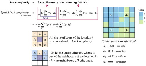
where $P_{i}$ is the spatial local complexity for a location ‘i’ and $G_{i}$ is the normalized indicator, i.e. the developed geocomplexity indicator in this study; W is a spatial adjacency matrix indicating the spatial relationship between observations. The adjacency matrix is represented by ‘0’ and ‘1’. When location ‘i’ and location ‘j’ are spatial neighbors, the value $W_{i j}$ is ‘1’. $Z_{i}$ is the standardized value (Z-score) of the selected factor at location ‘i’; $Z_{j}$ is the Z-score of the selected factor at location ‘j’, and ‘j’ is the spatial neighbor of the location ‘i’; $Z_{k}$ is the Z-score of the selected factor at location ‘k’, and ‘k’ is the spatial neighbor of both location ‘j’ and ‘i’, and {k} is a subset of {j}; m is the total number of spatial neighbors of location ‘i’; $v_{k}$ is the number of spatial neighbors of location ‘j’ while these neighbors for location ‘j’ should be spatial neighbors of location ‘i’ at the same time.

EquationEquation (1)(1) $_{P_{i}} = - \frac{1}{m} Z_{i} \sum_{j = 1}^{m} W_{i j} • Z_{j} - \frac{1}{m} \sum_{j = 1}^{m} W_{i j} • Z_{j} \frac{1}{v_{k}} \sum_{k = 1}^{n} {W_{j k} • W_{i k} • Z}_{k}$ (1) illustrates the computation of spatial local complexity using a spatial adjacency matrix, with the term ‘ $Z_{i} \sum_{j = 1}^{m} W_{i j} • Z_{j}$ ’ is based on a Moran measure for local spatial autocorrelation. This research makes further exploration by introducing the term ‘ $\sum_{j = 1}^{m} W_{i j} • Z_{j} \frac{1}{v_{k}} \sum_{k = 1}^{n} {W_{j k} • W_{i k} • Z}_{k}$ ’ to capture the surrounding local spatial dependence from the view of location ‘i’. This term calculates the product of Z-score in location ‘j’ (the spatial neighbor of location ‘i’) and Z-score in location ‘k’ (the spatial neighbor of both location ‘i’ and location ‘j’, and also the spatial neighbor of location ‘j’ restricted by spatial impact from location ‘i’). In other words, this term partially computes the local Moran value of location ‘j’. Only when the neighbor of ‘j’ is the neighbor of ‘i’ at the same time will location ‘k’ be considered in the computation. This computing strategy ensures that all computation results are related to the target location ‘i’. The value of ‘ $Z_{i} \sum_{j = 1}^{m} W_{i j} • Z_{j}$ ’ is positive when a majority of surroundings have the same sign (positive or negative) as the location ‘i’, indicating strong local autocorrelation. Similarly, when a majority of Z-scores in location ‘k’ have the same sign (positive or negative) as those in each of the locations ‘j’, the term ‘ $\sum_{j = 1}^{m} W_{i j} • Z_{j} \frac{1}{v_{k}} \sum_{k = 1}^{n} {W_{j k} • W_{i k} • Z}_{k}$ ’ has a high positive value, indicating strong autocorrelation among the surroundings. To balance the impact of surrounding autocorrelation with the main local spatial autocorrelation, a weighted average strategy is employed by dividing $v_{k}$ and m. The value of $\frac{1}{v_{k}}$ ensures that the impact of each surrounding autocorrelation does not exceed the impact of the main local spatial autocorrelation, while the value of $\frac{1}{m}$ ensures that the measure of spatial local complexity is not influenced by the number of neighboring observations.

EquationEquation (1)(1) $_{P_{i}} = - \frac{1}{m} Z_{i} \sum_{j = 1}^{m} W_{i j} • Z_{j} - \frac{1}{m} \sum_{j = 1}^{m} W_{i j} • Z_{j} \frac{1}{v_{k}} \sum_{k = 1}^{n} {W_{j k} • W_{i k} • Z}_{k}$ (1) can be simplified to EquationEquation (2)(2) $P_{i} = - \frac{1}{m} \sum_{j = 1}^{m} [Z_{i} • Z_{j} + \frac{1}{v_{k}} \sum_{k = 1}^{n} Z_{j} • Z_{k}]$ (2) under clear spatial relationships among ‘i’, ‘j’, and ‘k’. illustrates the relationships among three types of locations, with an example under the queen criterion. When the location ‘i’ is at the center of the square, the set of {j} refers to the eight surrounding squares. For each element in {j}, the corresponding sets of {k} and $v_{k}$ are different. For instance, when an element ‘j’ is located at the top of location ‘i’, the set of {k} consists of four squares marked in blue, and the value of $v_{k}$ is 4.

EquationEquation (1)(1) $_{P_{i}} = - \frac{1}{m} Z_{i} \sum_{j = 1}^{m} W_{i j} • Z_{j} - \frac{1}{m} \sum_{j = 1}^{m} W_{i j} • Z_{j} \frac{1}{v_{k}} \sum_{k = 1}^{n} {W_{j k} • W_{i k} • Z}_{k}$ (1) and EquationEquation (2)(2) $P_{i} = - \frac{1}{m} \sum_{j = 1}^{m} [Z_{i} • Z_{j} + \frac{1}{v_{k}} \sum_{k = 1}^{n} Z_{j} • Z_{k}]$ (2) employ the negative summation of local and surrounding features to measure spatial local complexity, where negative values represent more spatial complexity and lower values indicate less disorder. The negative measure of spatial features is consistent with the understanding of complexity, as a higher value indicates more spatial complexity. Areas with strong spatial dependence should exhibit similar Z-scores between the area and its surroundings, while regions with low geocomplexity are expected to have negative spatial local complexity values. For example, in , $A_{1}$ exhibits a relatively low spatial local complexity value and follows a pattern of spatial autocorrelation, while the surrounding patterns are simple. However, both local features and surrounding features from $A_{2}$ and $A_{4}$ are complex, as demonstrated in disorder against spatial dependence, resulting in corresponding spatial local complexity values that are positive or close to zero according to EquationEquation (1)(1) $_{P_{i}} = - \frac{1}{m} Z_{i} \sum_{j = 1}^{m} W_{i j} • Z_{j} - \frac{1}{m} \sum_{j = 1}^{m} W_{i j} • Z_{j} \frac{1}{v_{k}} \sum_{k = 1}^{n} {W_{j k} • W_{i k} • Z}_{k}$ (1) .

This research further normalizes the spatial local complexity in EquationEquation (3)(3) $G_{i} = \frac{P_{i} - \min (P_{i})}{\max (P_{i}) - \min (P_{i})}$ (3) to explain spatial error from traditional estimation models. As a region may have multiple spatial variables representing different attributes, the value range of the spatial local complexity of each variable may differ. The normalization process ensures that the value ranges of all relevant spatial local complexity from variables are the same and range from 0 to 1. This study uses normalized complexity to examine the extent to which spatial local complexity can explain unknown errors in linear models, machine learning models, and spatial heterogeneity models. Additionally, this study assesses to what extent the consideration of spatial local complexity could improve the performance of the GWR model.

3. Case study: determinants of nation-level economic inequality

Income inequality, which refers to the unequal distribution of income across different scales, is a form of economic disparity. This phenomenon has been on the rise in developed countries, including Australia, over the past decades (Athanasopoulos and Vahid Citation2003). Understanding economic disparity and the associated factors can benefit Australian national policy-making. Previous studies, dating back to 1960s, indicate that economic inequality is associated with various factors, such as gender, specific industry activities, education level, and employment (Murray Citation1978, Reeson et al. Citation2012, Fleming and Measham Citation2015). However, as circumstances have changed over time, the current association between economic inequality and socio-economic variables requires further investigation. The Gini coefficient is currently the most widely used inequality indicator, with acceptable properties of scale and size independence (Athanasopoulos and Vahid Citation2003). Detailed and precise information on the Gini coefficient at different spatial scales is accessible from the Australian Bureau of Statistics (ABS) source (Australian Bureau of Statistics Citation2020). Statistical Area Level 3 (SA3) is a spatial scale representing entire regions serviced by regional cities. Investigations conducted at this regional level can provide guidance for more detailed regional decision-making (Australian Bureau of Statistics Citation2016). To address gaps and provide potential value to policy-making, we conduct a case study on nationwide economic inequality and its associated factors at SA3 level in Australia. In this study, we introduce spatial local complexity as a spatial index to explain unknown residuals from traditional models.

3.1. Economic inequality data

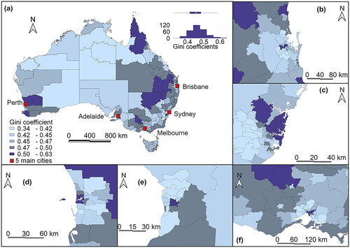
The Gini coefficient is a critical economic indicator measuring the inequality of income distribution (Cowell Citation2011, Mukhopadhyay and Sengupta, Citation2021). Its value ranges from 0 to 1, where 0 represents ideal economic equality and 1 indicates extreme inequality, with a coefficient over 0.5 indicating severe gaps in income distribution (Shorrocks Citation1978). Understanding the determinants and spatial patterns of economic inequality can assist regional planners in designing regions with more effective policies. In Australia, nationwide economic inequality data are available from the ABS based on census data. The Gini coefficient at the SA3 level, obtained from the government-maintained website (Australian Bureau of Statistics Citation2020), is used as a dependent variable in this study to indicate economic inequality. The 2016 census report indicates that 16% of SA3 regions have Gini coefficients above 0.5, and all regions with Gini coefficients above 0.55 are located in major cities (Australian Bureau of Statistics Citation2020). shows the distribution of economic inequality across Australia, with all five major cities containing regions with Gini coefficients greater than 0.5.

Figure 2. Spatial distributions of Gini coefficients in Australia (a) and major cities, including Brisbane (b), Sydney (c), Perth (d), Adelaide (e) and Melbourne (f).

Several factors may cause the unbalanced economic distribution, as indicated by the Gini coefficient. These factors include education, local income levels, gender, infrastructure development, and financial status of the community (Rodríguez-Pose and Tselios, Citation2010; Solga, Citation2014, Klenert et al. Citation2018, Liczbińska and Sobkowiak Citation2020). In addition to these factors, the industrial sector also plays a key role in economic development. Three key industries in Australia, including manufacturing, mining, and utility supply and waste service, contributed 25% of the national GDP in 2016 (Australian Bureau of Statistics Citation2018). A study has shown that industrialization also has impacts on wage inequality (Sbardella et al. Citation2017). Thus, industrial company, industrial employee scale, and industrial area scale may have an impact on economic inequality distribution. This study will explore the relationship between economic inequality and these influential variables. This study will also test the ability of geocomplexity to explain unknown residuals from traditional models by using different spatial matrices, which will be compared with another spatial index.

3.2. Explanatory data

The datasets containing potential explanatory variables in this study were sourced from ABS, OpenStreetMap (OSM), and National Pollutant Inventory (NPI), as demonstrated in . The study considers eight social and infrastructure variables that may be associated with economic inequality. These variables include sex ratio, internet accessibility rate, higher education level, median income level, house ownership rate, number of key industrial companies, and number of industrial employees. The data for these variables were sourced from ABS at the SA3 level in 2016 (Australian Bureau of Statistics Citation2020), under categories of population and people, income, education and employment, and family and community. The corresponding SA3 spatial boundaries were also obtained from the ABS data archives (Australian Bureau of Statistics Citation2016).

Table 1. A summary of explanatory variables.

Download CSV Display Table

Furthermore, this study also incorporates the industrial area scale as an independent variable. The industrial scale is calculated as the ratio of the total industrial area within the SA3 region to the corresponding SA3 area size. In this study, the industrial area encompasses regions and lands that are designed to support industrial activities such as manufacturing, mining and utility supply, and waste service. These industrial regions contain both land use planned for industrial activities and areas with a high density of industrial infrastructures. Industrial land uses are represented by OSM land use polygons tagged with ‘industrial’ in this study because the definition of OSM industry coincides with the three key industries under the scope of Australian industry (Australian Bureau of Statistics Citation2018). High-density industrial infrastructure areas are regions that have a number of relevant infrastructures recorded by the Australian government at NPI or outlined by OSM, and the infrastructure density is measured by a kernel density estimation approach. OSM-based land use polygon and industrial infrastructure data for the year 2016 are available on the OSM website (Geofabrik and OpenStreetMap contributors Citation2020). Industrial infrastructures recorded by the Australian government from NPI are available on the government-maintained website (Department of the Environment and Energy, Australian Government Citation2020). The identification of final industrial areas follows a validated spatial methodology based on Australian Statistical Geography Standards (ASGS) (Song et al., Citation2018, Zhang et al. Citation2022).

3.3. Experiment design

This research contains five key stages as demonstrated in . First, basic regression assumptions should be satisfied, which is indicated by the correlation test and multicollinearity test. Variables that satisfy regression assumptions, given the case study of economic inequality, are selected. Second, geocomplexities for selected determinants are computed based on the proposed definitions in Section 2. By applying further tests of regression assumptions, geocomplexities that are relevant to economic inequality are chosen. Next, three traditional models (i.e. multiple regression, SVR and GWR) are applied with optimized parameters to estimate nationwide economic inequality. These three selected regression models have been applied in various applications, given their properties. Multiple regression (i.e. linear regression) is the simplest and most commonly used model for estimation and prediction. SVR is the regression model with machine learning techniques, which has more power of explanation and has also been widely used (Nieto et al., Citation2021). GWR is one of the most commonly used regression techniques modeling geospatial information (Fotheringham Citation2002). These methods are selected as classic representatives of a regression model. Then, selected geocomplexities are utilized to estimate residuals from three regression models using GWR to measure to what extent different types of model errors can be explained by the spatial index. Finally, the power of error explanation of geocomplexity using the binary spatial matrix is compared with that of local Geary’s C and geocomplexity using row standardized matrix.

Figure 3. The workflow for assessing geocomplexity of economic inequality and its contribution to explaining spatial errors.

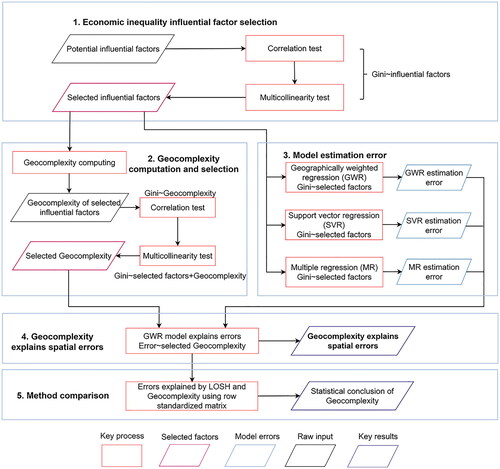
In this study, correlation tests and multicollinearity tests are applied to help select influential variables and complexities that satisfy regression assumptions from a number of candidate variables. The correlation test is the test of the Pearson correlation coefficient. A p-value greater than 0.05 for the Pearson correlation coefficient with the Gini coefficient indicates that the corresponding variable or geocomplexity is not statistically relevant to economic inequality. This study applied two multicollinearity tests indicated by variance inflation factor (VIF) value to diagnose the interrelation among variables and validate the basic regression assumption. A threshold of 2.5 is set for VIF value, indicating multicollinearity, and factors with VIF value higher than 2.5, indicating considerable collinearity, are filtered (Johnston et al. Citation2018). The multicollinearity test is applied twice in this study. The first multicollinearity test during the economic inequality factor selection process is applied to validate the regression assumption for selected influential factors. The second multicollinearity test for geocomplexity selection further diagnoses the inter-association among selected influential factors and their geocomplexities.

3.4. Models and errors

This study employs three models (i.e. multiple regression, support vector regression, and GWR) to investigate the relationship between economic inequality and determinants. For the multiple regression, model parameters are calculated based on the Least Squares using R packages. For the SVR model, optimal machine learning parameters, including the cost value and the gamma value, are determined by ten-fold cross-validation, and SVR estimation results are computed by the ‘e1071’ R language package. In this study, the cost of SVR is selected from all values from 0.1 to 100 with 0.1 as a step. For the GWR model, the optimal bandwidth is determined by cross-validation operated by the ‘spgwr’ R language package. Starting with an initial value from 0 to 1, the performance of bandwidth is assessed using leave-one-out cross-validation. The optimal bandwidth should have the best estimation performance, and the change of performance is small enough till the next iteration for searching. The GWR bandwidth in this study is adaptive based on k-nearest neighbors. The GWR model is applied to explain the cause of economic inequality with spatial concerns. At the final stage, selected geocomplexities will be applied to explain errors from these three models. The GWR model is a quantitative analysis approach representing the second law of geography, and this spatial method is further used to show to what extent spatial disparity of geocomplexity can explain errors from three traditional models.

4. Results

4.1. Determinants of economic inequality

Based on the correlation test, six variables, including higher education ratio, sex ratio, income, house ownership, industrial employee, and industrial scale, were initially identified as potential determinants of economic inequality. The multicollinearity test revealed that the higher education ratio had a high degree of collinearity with other factors, with a VIF value over 8, which is higher than the threshold value 2.5. To satisfy regression assumptions, the higher education ratio was removed, leaving the remaining five variables with VIF values lower than 2.5, including sex ratio, income, house ownership, industrial employee, and industrial scale, to be selected. shows the global coefficients and performance of the multiple regression model for the five selected determinants. The p-values for income, house ownership and industrial employee were less than 0.001, indicating their significant contributions to explaining economic inequality. The results suggest that a higher median income level, higher percentage of house ownership, and lower number of industrial employees could increase economic inequality. The general model with five selected factors is acceptable as indicated by the p-value for F-statistic. Spatial local complexities were computed for the five selected determinants, and relevant spatial local complexities were applied to explain unknown errors from three traditional models.

Table 2. Multiple regression for modelling Gini coefficients at the SA3 level.

Download CSV Display Table

4.2. Geocomplexity of explanatory variables

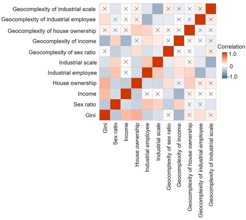
The correlation matrix in shows that spatial local complexities of income and industrial employees are correlated to economic inequality. The introduction of these two spatial local complexities does not cause the VIF values of the previously selected factors and the two correlated spatial local complexities to exceed the threshold of 2.5. Therefore, the spatial local complexities of income and industrial employees are then selected as influential geographical factors impacting economic inequality.

Figure 4. The correlation matrix among Gini coefficients selected explanatory variables, and geocomplexities of explanatory variables. Note: ‘x’ indicates that the correlation is not significant.

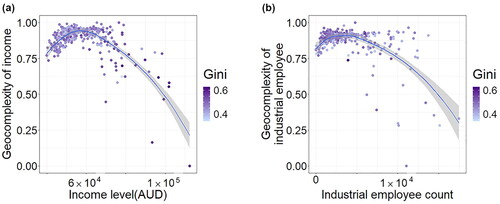
shows the statistical distributions of two selected spatial local complexities for factors compared with the corresponding factor values. The scatter plots show the distributions of income level and industrial employees against their local spatial complexity patterns, with each point representing an SA3 region. According to , higher spatial complexity of local income tends to locate in SA3 regions with low-medium income levels, and a similar trend is shown in the industrial employee count in . The findings suggest that regions with either very high or very low values of income or industrial employees tend to exhibit simple local spatial patterns, with those having the highest values displaying the most simple local spatial patterns. In contrast, regions with moderate values show the highest levels of geocomplexity.

Figure 5. Geocomplexity of selected variables in SA3 regions colored by Gini coefficient. (a) Income level v.s. Geocomplexity of income. (b) Industrial employee counts v.s. Geocomplexity of industrial employees.

4.3. Errors from three models

Three models, including multiple regression, SVR, and GWR, are applied to estimate nationwide economic inequality. Section 3.4 explains the process of determining model parameters. demonstrates the performance of the three models, while shows statistical distributions of estimation errors. Using the Least Squares method, multiple regression can explain 47% of the economic inequality. Using ten-fold cross-validation, the SVR model selects a cost value of 1.4 and a gamma value of 0.2 for the radial kernel as optimal parameters. With these optimal parameters, the SVR model can explain 65% of the economic inequality. By applying cross-validation for the adaptive bandwidth selection, the GWR estimation performs the best among the three models with an R² of 76%.

Figure 6. Statistical distribution of model errors. (a) Errors of multiple regression estimations. (b) Errors of SVR estimations. (c) Errors of GWR estimations.

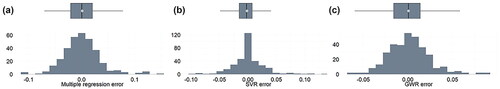
Table 3. Performance of three models.

Download CSV Display Table

4.4. Geocomplexity explains spatial errors

4.4.1. Overview of explaining spatial errors using geocomplexity

This research aims to further investigate the extent to which spatial local complexities can explain estimation errors of traditional models, and how selected geocomplexities can explain spatial errors. Considering the spatial variation of geography impacts, we used GWR to quantify the explanation of selected spatial local complexities on estimation errors. shows the statistical summaries of the significant results of three error explanation models based on GWR. The spatial disparity of selected complexities can explain 47% of linear regression errors, 17% of SVR regression errors, and 14% of GWR errors. The residual-fitted plots of error explanation models are shown in , and residuals are randomly distributed around the horizontal line of 0 without significant linear or non-linear patterns. Thus, there is no significant non-linear or heteroscedasticity problem for the three explanation models. Q-Q plots from demonstrate probability distributions of residuals from three error explanations compared with randomly generated data with normal distribution. For residuals from multiple regression and GWR error explanation models, a majority of points fall on the reference line as shown in .

Figure 7. Residuals of error explanations. (a) Residual-fitted plot of error explanation from three models. (b) Q-Q plot showing residuals of multiple regression error explanation. (c) Q-Q plot showing residuals of SVR error explanation. (d) Q-Q plot showing residuals of GWR error explanation.

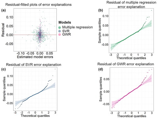
Table 4. A summary of the contribution of geocomplexity in explaining spatial errors.

Display Table

4.4.2. Spatial explanation of multiple regression errors by geocomplexities

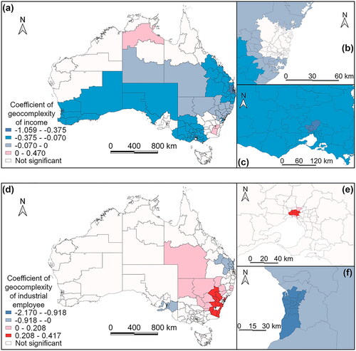
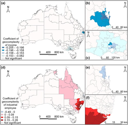
demonstrates how estimation errors from multiple regression can be spatially explained by selected spatial local complexities. The spatial local complexity of income and industrial employees can significantly explain linear errors in many regions in the Australian continent. The spatial local complexity of income is positively significant in Northern Territory and remote areas of New South Wales, while the geocomplexity coefficient is negatively significant in a majority of regions, including Melbourne, Brisbane, Perth as well as other inner regional and remote areas. demonstrates the explanation of geocomplexity in Sydney’s surrounding regions, and shows that the spatial explanation for linear errors varies in Melbourne. The spatial local complexity of industrial employees is positively significant in Melbourne and the inner region of New South Wales and Brisbane, but negatively significant in Adelaide and surrounding regions.

Figure 8. Coefficients of geocomplexity of income and industrial employee in multiple regression error explanation. Distribution of geocomplexity of income in Australia (a) and major cities including, Sydney (b) and Melbourne (c). Distribution of geocomplexity of industrial employees in Australia (d) and major cities including, Melbourne (e) and Adelaide (f).

4.4.3. Spatial explanation of support vector regression errors by geocomplexities

illustrates how spatial local complexity can explain errors from SVR estimations. As a result, significant results are distributed in the East part of the continent. Spatial local complexity of income is negatively associated with SVR errors, and significant results of income complexity are clustering in Melbourne and Brisbane as shown in . Furthermore, the higher absolute value of the coefficient in Brisbane indicates that SVR errors are more sensitive to the change of spatial impact in Brisbane and surrounding areas. In terms of spatial local complexity of industrial employees, a majority of significant results demonstrate a positive relation, and a small number of negative significant results are distributed in the Northern Greater Brisbane Area as shown in . The positive significant coefficient of spatial local complexity of industrial employees is higher in the Southern of the continent.

Figure 9. Coefficients of geocomplexity of income and industrial employee in SVR error explanation. Distribution of geocomplexity of income in Australia (a) and major cities including, Brisbane (b) and Melbourne (c). Distribution of geocomplexity of industrial employees in Australia (d) and major cities including, Brisbane (e) and Sydney (f).

4.4.4. Spatial explanation of geographically weighted regression errors by geocomplexities

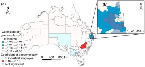
The spatial disparity of two selected complexities can also further explain the remaining errors from the GWR model only concerning five influential factors. As shown in , spatial local complexity of income is negatively associated with GWR errors in 53 SA3 areas and spatial local complexity of industrial employees is positively associated with GWR errors in three SA3 areas in New South Wales. Significant results of spatial local complexity of income are distributed in the surrounding inner regions of the Greater Brisbane Area as shown in . The absolute value of the income complexity coefficient is higher in regions close to Brisbane than in other regions in Victoria and South Australia.

Figure 10. Coefficients of geocomplexity of income and industrial employee in GWR error explanation (a). Distribution of geocomplexity of income in Brisbane (b).

4.5. Method comparison

Our study proposes a new spatial index named ‘geocomplexity’, which indicates the pattern of spatial local complexity based on a Moran’s measure. This index is composed of LISA and all spatial associations between connecting neighbors of the target area with Moran’s measure. This spatial index is derived from and naturally connected to the local autocorrelation index. In this section, we add further tests, given the same case study of the association between Gini coefficient and independent variables shown in Section 3, using local autocorrelation represented by local Geary’s C and geocomplexity with row standardized spatial weight matrix to explain errors from three traditional models. Further tests follow the same workflow and criteria of factor selection as shown in . As a result, two spatial indexes for both income and industrial employees, identical to factor selection results in Section 3, are selected to explain errors from three models.

The performances in terms of the power of error explanation using three spatial indexes are shown in . Errors from three traditional models are explained by spatial indexes of local income level and industrial employee count. Geocomplexity with binary spatial weight matrix, with detailed results demonstrated in Section 3, has the best power of explanation for errors among all three methods. By replacing with row standardized spatial weight matrix for the computation of geocomplexity, the power of error explanation decreases. Geocomplexity with a row standardized matrix can explain more linear regression errors than local Geary’s C, but the power of explanation for the other two model errors is no different from that of local autocorrelation. Both geocomplexity and local autocorrelation are localized variables and they perform better using local regression models.

Table 5. The comparison between geocomplexity and local autocorrelation index on error explanation.

Display Table

5. Discussion

This study proposes a spatial index to measure the concept of complexity regarding spatial dependence. As geospatial impacts are not constant across space, the spatial complexity may vary in different places. Therefore, this research applies GWR models to quantify the spatial association between economic inequality and selected variables and explain unknown errors from traditional models by capturing local complexities. The aim of a series of experiments is to examine whether the consideration of spatial local complexity could explain more unknown errors from traditional models and improve model performance. As a result, this assumption is validated.

The power of error illumination from spatial local complexity is also compared with spatial autoregressive models, given the case study of economic inequality estimation. The Lagrange multiplier test of spatial dependence indicates that the spatial error model (SER) is the most suitable among spatial autoregressive models. With a p-value in F-statistics less than 0.001, the SER has an R-squared value of 0.64, indicating the fact that spatial autocorrelation of the error term can explain 32% of the original error. Thus, geocomplexity with either binary or row-standardized spatial matrix can explain more errors. It is worth noting that the concept of geocomplexity in our study is more compatible with a symmetric spatial matrix, given our definition. As shown in and EquationEquations (1)(1) $_{P_{i}} = - \frac{1}{m} Z_{i} \sum_{j = 1}^{m} W_{i j} • Z_{j} - \frac{1}{m} \sum_{j = 1}^{m} W_{i j} • Z_{j} \frac{1}{v_{k}} \sum_{k = 1}^{n} {W_{j k} • W_{i k} • Z}_{k}$ (1) and Equation(2)(2) $P_{i} = - \frac{1}{m} \sum_{j = 1}^{m} [Z_{i} • Z_{j} + \frac{1}{v_{k}} \sum_{k = 1}^{n} Z_{j} • Z_{k}]$ (2) , we consider the spatial dependence between neighbors of the target area as a mutual relationship. In other words, the connection status from location ‘j’ to ‘k’ (or ‘i’ to ‘k’) and ‘k’ to ‘j’ (or ‘k’ to ‘i’) is preferred to be identical. The main purpose of geocomplexity is to further include associations among neighbors when considering spatial dependence and additional information from the row standardized process cannot be reflected.

This research aims to provide an innovative understanding of complexity by extending the understanding of spatial dependence. The geocomplexity is a Moran-based measure (i.e. the multiplication of the Z-score of observations). We also analyzed different measures representing differences between observations including Geary’s C measure (i.e. the square of the difference between two values). As a result, the Moran-based measure performs better. Despite the stronger power of error illumination, the spatial local complexity may not be the final or the only answer to the question ‘what is complexity in spatial science’. We redefine the concept of ‘spatial complexity’ considering spatial dependence between neighbors, and this could not be the only definition. For instance, the ‘spatial complexity’ can also be redefined considering the third law of geography, which defines a concept of ‘spatial similarity’ that the target variable between two locations is similar if geographic configurations at these two places are identical (Zhu et al. Citation2018, Song Citation2022b). That means a region can be spatially complex where geographic configurations are not closely associated. In future work, the content of ‘complexity’ under the spatial scope can be filled by other meaningful spatial concepts. In terms of further application, geocomplexity can also be a complexity measure in future remote sensing studies, especially hyperspectral image unmixing (Jia and Qian 2017). Last but not the least, in future studies, spatial filtering tools can be a method supporting geospatial information modeling along with spatial local complexity. The applications of spatial filtering for selecting influential variables together with geocomplexity for error explanation have the potential to explore the limits of spatial data modeling (Paez Citation2019).

6. Conclusion

This study proposes a spatial index named ‘geocomplexity’ to measure the concept of complexity regarding spatial dependence. The index demonstrates the complexity of spatial dependence by considering both the relationship between an interested area and surroundings, and the associations among spatial neighbors of the target area. Given a case study of the association between nationwide economic inequality and influential variables, results show that spatial local complexity can explain unknown errors and improve the traditional model performance. This index can be an indicator quantifying the phenomenon of complexity for factors from the view of spatial dependence. The index with local regression can be a further explanation for regression analysis methods, and spatial locations with significant results from error explanations may indicate considerate dependence among local neighbors. The proposed spatial complexity index is suited well to a symmetric spatial weight matrix and geocomplexity with binary spatial weight matrix has better power of error explanation than geocomplexity with asymmetric matrix and local Geary’s C. The proposed geocomplexity indicator has the potential for spatial data analysis and relevant applications in both implying complexity in spatial science and illuminating unknown errors from traditional models.

Acknowledgements

We thank the editor and anonymous reviewers for their valuable comments and suggestions for improving the quality of this manuscript.

Data and codes availability statement

The data and code that support the findings of this study are available in Figshare at https://doi.org/10.6084/m9.figshare.20500284.v1.

Disclosure statement

No potential conflict of interest was reported by the author(s).

References

Anselin, L., 2019. A local indicator of multivariate spatial association: Extending geary’s c. Geographical Analysis, 51 (2), 133–150.
Web of Science ®Google Scholar
Athanasopoulos, G., and Vahid, F., 2003. Statistical inference and changes in income inequality in Australia. Economic Record, 79 (247), 412–424.
Web of Science ®Google Scholar
Australian Bureau of Statistics., 2016. Australian Statistical Geography Standard (ASGS): Volume 1 - Main Structure and Greater Capital City Statistical Areas, July 2016. [online]. Available from: https://www.abs.gov.au/AUSSTATS/[email protected]/DetailsPage/1270.0.55.001July%202016?OpenDocument
Google Scholar
Australian Bureau of Statistics., 2018. Australian Industry [online]. Available from: https://www.abs.gov.au/AUSSTATS/[email protected]/DetailsPage/8155.02016-17?OpenDocument
Google Scholar
Australian Bureau of Statistics., 2020. Data by region [online]. Available from https://www.abs.gov.au/AUSSTATS/[email protected]/DetailsPage/1410.02014-19?OpenDocument
Google Scholar
Batty, M., et al., 2014. Entropy, complexity, and spatial information. Journal of Geographical Systems, 16 (4), 363–385.
PubMed Web of Science ®Google Scholar
Chi, G., and Zhu, J., 2008. Spatial regression models for demographic analysis. Population Research and Policy Review, 27 (1), 17–42.
Web of Science ®Google Scholar
Cola, L.D., 1994. Simulating and mapping spatial complexity using multi-scale techniques. International Journal of Geographical Information Systems, 8 (5), 411–427.
Web of Science ®Google Scholar
Cowell, F.A., 2011. Measuring Inequality. Oxford: Oxford University Press.
Google Scholar
Department of the Environment and Energy, Australian Government., 2020. National Pollutant Inventory [online]. Available from: http://www.npi.gov.au/npidata/action/load/browse-search/criteria/browse-type/Industry/year/2016
Google Scholar
Epperson, B.K., and Li, T., 1996. Measurement of genetic structure within populations using Moran’s spatial autocorrelation statistics. Proceedings of the National Academy of Sciences of the United States of America, 93 (19), 10528–10532.
PubMed Web of Science ®Google Scholar
Fleming, D.A., and Measham, T.G., 2015. Income Inequality across Australian Regions during the Mining Boom: 2001–11. Australian Geographer, 46 (2), 203–216.
Web of Science ®Google Scholar
Fotheringham, A.S., 2002. Geographically weighted regression: The analysis of spatially varying relationships. Chichester: John Wiley & Sons.
Google Scholar
Geofabrik and OpenStreetMap contributors., 2020. Download OpenStreetMap for this region: Australia and Oceania [online]. Available from: http://download.geofabrik.de/australia-oceania.html
Google Scholar
Henebry, G.M., 1995. Spatial model error analysis using autocorrelation indices. Ecological Modelling, 82 (1), 75–91.
Web of Science ®Google Scholar
Ilunga, M., 2019. Shannon entropy for measuring spatial complexity associated with mean annual runoff of tertiary catchments of the Middle Vaal basin in South Africa. Entropy (Entropy), 21 (4), 366.
PubMed Web of Science ®Google Scholar
Jia, S., and Qian, Y., 2007. Spectral and spatial complexity-based hyperspectral unmixing. IEEE Transactions on Geoscience and Remote Sensing: A Publication of the IEEE Geoscience and Remote Sensing Society, 45 (12), 3867–3879.
Web of Science ®Google Scholar
Johnston, R., Jones, K., and Manley, D., 2018. Confounding and collinearity in regression analysis: a cautionary tale and an alternative procedure, illustrated by studies of British voting behaviour. Quality & Quantity, 52 (4), 1957–1976.
PubMedGoogle Scholar
Klenert, D., et al., 2018. Infrastructure and inequality: Insights from incorporating key economic facts about household heterogeneity. Macroeconomic Dynamics, 22 (4), 864–895.
Web of Science ®Google Scholar
Liczbińska, G., and Sobkowiak, A., 2020. Did the sex ratio at birth reflect social and economic inequalities? The pilot study from the Poznań province, 1875–1913. Przeszłość Demograficzna Polski, 42, 95–121.
Google Scholar
Luo, P., et al., 2023. A generalized heterogeneity model for spatial interpolation. International Journal of Geographical Information Science, 37 (3), 634–659.
Web of Science ®Google Scholar
Mukhopadhyay, N., and Sengupta, P.P., eds. 2021. Gini Inequality Index: Methods and Applications. Boca Raton, FL: CRC Press.
Google Scholar
Murray, D., 1978. Sources of income inequality in Australia, 1968-69. Economic Record, 54 (2), 159–169.
Google Scholar
Nieto, D.M.C., Quiroz, E.A.P., and Lengua, M.A.C., 2021. A systematic literature review on support vector machines applied to regression. 2021 IEEE Sciences and Humanities International Research Conference (SHIRCON).
Google Scholar
Owers, C.J., Rogers, K., and Woodroffe, C.D., 2016. Identifying spatial variability and complexity in wetland vegetation using an object-based approach. International Journal of Remote Sensing, 37 (18), 4296–4316.
Web of Science ®Google Scholar
Paez, A., 2019. Using spatial filters and exploratory data analysis to enhance regression models of spatial data: Using spatial filters and exploratory data analysis. Geographical Analysis, 51 (3), 314–338.
Web of Science ®Google Scholar
Poudyal, N.C., Butler, B.J., and Hodges, D.G., 2019. Spatial analysis of family forest landownership in the southern United States. Landscape and Urban Planning, 188, 163–170.
Web of Science ®Google Scholar
Pringle, M.J., and Lark, R.M., 2006. Spatial analysis of model error, illustrated by soil carbon dioxide emissions. Vadose Zone Journal, 5 (1), 168–183.
Web of Science ®Google Scholar
Reeson, A.F., Measham, T.G., and Hosking, K., 2012. Mining activity, income inequality and gender in regional Australia: Mining activity, income inequality and gender. Australian Journal of Agricultural and Resource Economics, 56 (2), 302–313.
Web of Science ®Google Scholar
Rodríguez-Pose, A., and Tselios, V., 2010. Inequalities in income and education and regional economic growth in Western Europe. The Annals of Regional Science, 44 (2), 349–375.
Web of Science ®Google Scholar
Rufino, M.M., Bez, N., and Brind’Amour, A., 2020. Ability of spatial indicators to detect geographic changes (shift, shrink and split) across biomass levels and sample sizes. Ecological Indicators, 115, 106393.
Web of Science ®Google Scholar
Sbardella, A., Pugliese, E., and Pietronero, L., 2017. Economic development and wage inequality: A complex system analysis. PloS One, 12 (9), e0182774
PubMed Web of Science ®Google Scholar
Shorrocks, A., 1978. Income inequality and income mobility. Journal of Economic Theory, 19 (2), 376–393.
Web of Science ®Google Scholar
Solga, H., 2014. Education, economic inequality and the promises of the social investment state. Socio-Economic Review, 12 (2), 269–297.
Web of Science ®Google Scholar
Song, Y., et al., 2018. Are all cities with similar urban form or not? Redefining cities with ubiquitous points of interest and evaluating them with indicators at city and block levels in China. International Journal of Geographical Information Science, 32 (12), 2447–2476.
Web of Science ®Google Scholar
Song, Y., and Wu, P., 2021. An interactive detector for spatial associations. International Journal of Geographical Information Science, 35 (8), 1676–1701.
Web of Science ®Google Scholar
Song, Y., 2022a. The second dimension of spatial association. International Journal of Applied Earth Observation and Geoinformation, 111, 102834.
Web of Science ®Google Scholar
Song, Y., 2022b. Geographically Optimal Similarity. Mathematical Geosciences, 55 (3), 295–320.
Web of Science ®Google Scholar
Suh, N.P., 1999. A theory of complexity, periodicity and the design axioms. Research in Engineering Design, 11 (2), 116–132.
Web of Science ®Google Scholar
Weisent, J., et al., 2012. Socioeconomic determinants of geographic disparities in campylobacteriosis risk: a comparison of global and local modeling approaches. International Journal of Health Geographics, 11 (1), 45.
PubMedGoogle Scholar
Yanovski, R., Nelson, P.A., and Abelson, A., 2017. Structural complexity in coral reefs: Examination of a novel evaluation tool on different spatial scales. Frontiers in Ecology and Evolution, 5, 27.
Web of Science ®Google Scholar
Zhang, Z., Song, Y., and Wu, P., 2022. Robust geographical detector. International Journal of Applied Earth Observation and Geoinformation, 109, (102782.
Web of Science ®Google Scholar
Zhu, A.-X., et al., 2018. Spatial prediction based on third law of geography. Annals of GIS, 24 (4), 225–240.
Web of Science ®Google Scholar

Geocomplexity explains spatial errors

Abstract

1. Introduction

2. Spatial local complexity