Incorporating multimodal context information into traffic speed forecasting through graph deep learning

Abstract

Accurate traffic speed forecasting is a prerequisite for anticipating future traffic status and increasing the resilience of intelligent transportation systems. However, most studies ignore the involvement of context information ubiquitously distributed over the urban environment to boost speed prediction. The diversity and complexity of context information also hinder incorporating it into traffic forecasting. Therefore, this study proposes a multimodal context-based graph convolutional neural network (MCGCN) model to fuse context data into traffic speed prediction, including spatial and temporal contexts. The proposed model comprises three modules, ie (a) hierarchical spatial embedding to learn spatial representations by organizing spatial contexts from different dimensions, (b) multivariate temporal modeling to learn temporal representations by capturing dependencies of multivariate temporal contexts and (c) attention-based multimodal fusion to integrate traffic speed with the spatial and temporal context representations for multi-step speed prediction. We conduct extensive experiments in Singapore. Compared to the baseline model (spatial-temporal graph convolutional network, STGCN), our results demonstrate the importance of multimodal contexts with the mean-absolute-error improvement of 0.29 km/h, 0.45 km/h and 0.89 km/h in 30-min, 60-min and 120-min speed prediction, respectively. We also explore how different contexts affect traffic speed forecasting, providing references for stakeholders to understand the relationship between context information and transportation systems.

Keywords:

• Traffic speed forecasting
• spatial context
• temporal context
• multimodal context fusion
• graph deep learning

1. Introduction

In high-density cities, the rapid growth of human mobility and daily activities has caused tremendous pressure on urban traffic, which in turn puts forward new requirements for transportation resilience when encountering severe traffic accidents (Haraguchi et al. 2022). Traffic speed forecasting is a prerequisite for achieving the resilience goal to anticipate future variations of traffic indicators (Kurth et al. 2020, Wang et al. 2020). The forecasting information of traffic indicators also enables a more evidence-based decision-making process in handling traffic congestion (Lana et al. 2018, Yin et al. 2022). Therefore, accurate traffic speed forecasting plays a vital role in alleviating traffic congestion and establishing intelligent transportation systems (Lana et al. 2018).

Human mobility occurs in situation-dependent settings that can be affected by extensive external factors, such as land use, transportation networks and weather conditions (Buchin et al. 2012). These factors belong to the scope of context information ubiquitously distributed over the urban environment. In the big data era, lots of sensors and platforms provide massive context data from various sources to boost urban traffic and human mobility research (Li et al. 2016, Tu et al. 2020b). For example, point of interest (POI) data from crowdsourcing depict the spatial distribution of interesting locations with attributes to help predict the next locations (Zhao et al. 2020); weather condition data from weather observation stations provide real-time meteorological information to help predict traffic information under different meteorological events (Jiang and Luo 2022). These multiple sources endow context data with multiformity in modalities (Lahat et al. 2015). Rather than using the traditional modality division, this study suggests dividing the data into spatial and temporal contexts to better exploit the spatio-temporal characteristics inherent in context data. POI and weather data are two representative examples of spatial and temporal contexts, respectively. By virtue of the ubiquitous distribution of context information, human mobility is simultaneously motivated and restricted by these context data anytime and anywhere (Sharif and Alesheikh 2017, Zhang and Raubal 2022). Hence, it is necessary to explore how to incorporate multimodal context data into traffic speed forecasting when taking their spatio-temporal characteristics into account.

Despite the necessity and importance of multimodal context data, two problems are encountered when using context information to promote traffic speed forecasting, ie (i) the difficulty of fusing multimodal context data and (ii) the challenge of incorporating the fused context representations into prediction. The first problem falls into exploring the mechanism of fusing multimodal context data with different dimensions, distributions and granularities (Lahat et al. 2015). Although multimodal context data furnish multifaceted and complementary situation information, there is a lack of effective tools to fuse these context data to sense the urban environment (Liu et al. 2020). For example, since POI and land use are distributed in urban areas with different spatial dimensions, the following question is raised: how to combine POI with land use to generate a fused representation for downstream tasks? In this situation, POI is a point-based dataset discretely distributed around the road network, while land use is a plane-based dataset continuously distributed over the urban space, making it challenging to fuse these two cross-dimensional datasets. A much more complicated scenario would occur when fusing spatial contexts with temporal contexts due to the involvement of the time dimension (Gao et al. 2020, Li and Zhu 2021). The second problem focuses on finding a solution to incorporate the fused context representations into existing state-of-the-art models of traffic speed prediction. So far, deep learning techniques have been widely used to improve the performance of traffic forecasting (Jiang and Luo 2022, Yin et al. 2022), such as recurrent neural network (RNN), graph neural network (GNN) and other variants. However, the exploration of using context information to boost traffic speed forecasting is still at a preliminary stage. A previous context-aware attempt proposed by Chen et al. (2020) focuses on spatio-temporal relationship exploration on graph sequences and utilizes graph convolutional neural networks to capture geographic-semantic-temporal contexts for traffic flow forecasting. Although this work achieves satisfactory performance in forecasting traffic flows, they did not explore the mechanism of incorporating external context factors (eg POIs, land use and weather) into prediction. Therefore, investigating how to fuse multimodal context data and incorporate them into traffic speed forecasting is of great significance to advance context-based intelligent transportation (Wang et al. 2018, Demšar et al. 2021) and GeoAI research (Janowicz et al. 2020).

In this study, we handle these two problems by proposing a multimodal context-based graph convolutional neural network (MCGCN) model to fuse multifaceted context information, including spatial and temporal contexts. Then, we utilize the fused context representations to improve traffic speed forecasting through an attention technique. Overall, our contributions are four-fold:

• We propose a hierarchical spatial embedding module to organize spatial contexts from various dimensions and learn spatial context representations, which can improve prediction accuracy compared to the non-hierarchical method.

• We propose a multivariate temporal modeling module to generate representations by capturing latent dependencies of multivariate temporal contexts. Using the generated temporal context representations to predict traffic speed outperforms the baseline method.

• To fuse multimodal contexts, we design an attention fusion layer to integrate traffic speed with spatial and temporal context representations for traffic speed forecasting. The experiments justify the feasibility and effectiveness of the proposed MCGCN model.

• This study reveals the significance of context information and explores how different contexts affect traffic speed forecasting.

The remainder of this paper is organized as follows. Section 2 reviews previous work on traffic forecasting and context-based human mobility research. In Section 3, we introduce the proposed MCGCN model and its technical details. Data processing and experimental results are reported in Sections 4 and 5, respectively. Finally, we conclude the paper and offer insights on future work in Section 6.

2. Related work

2.1. Traffic forecasting and deep learning

Traffic forecasting refers to the prediction of traffic information for a certain period using historical data, which is an important component of intelligent transportation systems (Lana et al. 2018, Kumar and Raubal 2021). The range of traffic information varies based on the particular prediction task but generally encompasses some commonly-used indicators, such as traffic flow, traffic speed and travel time (Yin et al. 2022). The essence of predicting these traffic indicators is to infer their trend, periodicity and dependency from a spatio-temporal perspective across the transportation network (Ermagun and Levinson 2018). In actual applications, traffic forecasting is of great significance to improve the resilience of transportation systems, such as mitigating traffic congestion and providing foreseeable prediction of traffic accidents in an emergency (Wu et al. 2018, Jiang and Luo 2022).

Many approaches have flourished to forecast short-term or long-term traffic information in the last decades, such as statistical, machine learning and deep learning methods (Tedjopurnomo et al. 2020, Kumar and Raubal 2021). Statistical methods were initially developed for traffic prediction from a time-series perspective, such as historical average, auto-regressive integrated moving average and vector autoregression (Han and Song 2003, Ermagun and Levinson 2018). However, these methods particularly suit small datasets and require data to meet certain assumptions that are complex for time-varying traffic information (Yin et al. 2022). Another kind of method is using machine learning models to predict traffic information through training massive historical data samples, such as random forest and support vector regression (Cheng et al. 2017, Liu and Wu 2017). Compared to statistical methods, machine learning models can process high-dimensional data and handle the nonlinear relationship of traffic information with better prediction performance (Li and Shahabi 2018). With the development of deep learning, recurrent neural network (RNN) has become one of the mainstream methods in traffic forecasting due to its ability to capture long-term dependencies of sequential traffic data that traditional machine learning methods are not good at capturing (Ramakrishnan and Soni 2018, Kashyap et al. 2022). Additionally, the variants of RNN-based models, such as the long short-term memory (LSTM) and gated recurrent unit (GRU), outperform the typical RNN models in traffic prediction by introducing the gate mechanism (Fu et al. 2016, Liu et al. 2017).

Although the RNN-based deep learning models show great potential in time-series prediction, they fail to model the spatial dependency of traffic prediction since the traffic information of a road segment is also affected by its neighboring road segments (Lana et al. 2018). To handle this problem, numerous studies have made great progress in developing models able to simultaneously capture spatial and temporal dependencies of traffic information, such as hybrid models and graph neural network (GNN). (Diao et al. 2019, Yin et al. 2022, Zhao et al. 2022). For example, Ren et al. (2020) proposed a hybrid deep learning model that integrates LSTM and convolutional neural network (CNN) to exploit their advantages in capturing spatial and temporal dependencies for citywide spatio-temporal flow prediction, yielding a high accuracy. Nonetheless, the applicability of CNN-based hybrid models to transportation networks is constrained by the graph structure inherent to such networks, thereby hindering their effectiveness in the realm of traffic forecasting (Li and Shahabi 2018, Kashyap et al. 2022). The emergence of GNN-based models solves this problem by modeling the spatio-temporal dependencies of traffic information in the transportation network through a graph structure (Jiang and Luo 2022), such as diffusion convolution recurrent neural network (DCRNN) (Li et al. 2017), spatial-temporal graph convolutional network (STGCN) (Yu et al. 2017a) and multivariate time-series graph neural network (MTGNN) (Wu et al. 2020). These GNN-based models have become state-of-the-art methods in traffic forecasting, which constitute the foundation of this study for speed prediction.

2.2. Context-based human mobility research

Context awareness has attracted considerable attention in human mobility research due to its ability to provide situation-specific information for transportation applications (Sattar et al. 2016). Essentially, individual movement distributed in road networks is simultaneously motivated and restricted by its surrounding context information (Sharif and Alesheikh 2017, Zhang and Raubal 2022). Therefore, developing context-based methods possesses potential gains to improve the understanding of human mobility patterns and the performance of traffic forecasting.

Despite the importance of context information, existing studies mostly use raw traffic information in the prediction task (Lana et al. 2018). This is due to the fact that the diversity and complexity of context information deepen the difficulty of incorporating it into traffic forecasting (Tedjopurnomo et al. 2020). Context diversity manifests itself in multiple modalities, and each modality may have its unique data source, dimension and distribution (Lahat et al. 2015). After summarizing previous research, this study proposes to divide context information into two modalities, ie spatial and temporal contexts. The spatial context pertains to static datasets containing geographical coordinates that describe the surrounding information of targeted entities. This context is ubiquitously distributed across the urban landscape in various dimensions, for example, POIs as zero-dimensional points, road networks as one-dimensional lines and land use as two-dimensional planes. These datasets aid in characterizing individual surrounding environments that may influence travel behaviors and preferences (Buchin et al. 2012, Lee and Holme 2015). The temporal context, on the other hand, refers to time-series situational information of targeted entities as it evolves over time. Taking traffic speed as a target example, time-series features related to the running of transportation systems fall under this context, such as time, traffic jams and weather conditions. Specifically, Huang and Wong (2015) discussed how temporal information influences individual movement by differentiating between days of the week, hours of the day and so on. Weather information can also have a significant impact, particularly during extreme meteorological events (Koesdwiady et al. 2016, Yu et al. 2017b). Overall, multimodal contexts cover an extensive scope of geographical and transportation-related factors with different modalities, posing a challenge of effectively exploiting context data in the traffic prediction task.

To handle this challenge, several studies have utilized context information to improve the performance of traffic forecasting (Yin et al. 2022). These studies provide a possibility to increase traffic prediction accuracy by integrating traffic indicators with surrounding context information, such as exploring the impact of land use changes on predicting traffic indicators (Azad and Wang 2021), improving speed prediction through exploiting temporal auxiliary information (Lin et al. 2018) and incorporating daily weather information into long-term traffic flow forecasting (Belhadi et al. 2020). However, the above-mentioned studies mainly focus on one kind of context information from either the spatial or temporal perspective regardless of their combined effects on prediction. Exploring the mechanism to fuse multimodal contexts is still an open problem in GeoAI and transportation research. In addition, the extents of spatial and temporal contexts are diverse and complicated, which also hinders fusing these contexts into combined representations for traffic speed forecasting. An early exploration by Ge et al. (2019a) proposed temporal graph convolutional networks to integrate social factors (eg day of the week) and geographical features (eg POI) into traffic speed prediction, but it still lacks a framework for summarizing and modeling multimodal context data. This study aims to solve the problem by proposing a multimodal context-based model to fuse traffic speed with spatial and temporal contexts and improve the performance of traffic prediction. Due to the difficulty of covering all context information in the urban environment, we chose several representative spatial and temporal contexts as an example to verify the feasibility of the proposed model.

3. Methodology

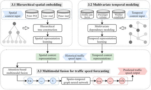
This study proposes a multimodal context-based graph convolutional neural network (MCGCN) model to fuse multifaceted context information and exploit the fused context representations to improve traffic speed forecasting. The MCGCN model consists of three modules, including hierarchical spatial embedding, multivariate temporal modeling and attention-based multimodal fusion. (a) For hierarchical spatial embedding, we construct a three-level tree for each road segment to organize spatial context data from different dimensions, ie points, lines and planes, and then utilize hierarchical graph learning to learn spatial context representations for each tree, ie S. (b) To capture latent dependencies of temporal contexts, the multivariate temporal modeling module automatically learns subgraphs of multivariate temporal contexts over different road segments, then employs graph convolution to produce temporal context representations based on the built subgraphs. For each road segment, its temporal context representations at the time step t can be expressed as ${\mathit{T}}^t.$ (c) Finally, an attention-based multimodal fusion module is proposed to integrate traffic speed (${\mathit{V}}^t$) with spatio-temporal context representations (S and ${\mathit{T}}^t$) and then fuse them into a graph convolutional network for multi-step speed prediction. An overview of this proposed MCGCN model is shown in Figure 1.

Figure 1. An overview of the proposed MCGCN model for traffic speed forecasting. It consists of three modules, including hierarchical spatial embedding, multivariate temporal modeling and attention-based multimodal fusion.

3.1. Hierarchical spatial embedding

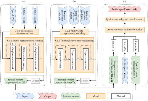
Geographical phenomena encounter the scale problem that influences the measurement of their properties across space (Ge et al. 2019b). To mitigate this problem, Tu et al. (2020a) explored the possibility of using multi-source geospatial data to portray urban land use from a hierarchical perspective, which can more comprehensively exploit the spatial and attribute information. Spatial pyramid pooling has also been developed in convolutional neural networks (He et al. 2015) and applied in representing spatial scenes (Guo et al. 2022). Accordingly, this study constructs a three-level tree to associate spatial context data from different dimensions and uses hierarchical graph learning to learn spatial representations (Ying et al. 2018). The architecture of hierarchical spatial embedding is demonstrated in Figure 2(a), which consists of (i) hierarchical tree construction for spatial contexts and (ii) spatial representation learning.

Figure 2. The architecture of the proposed MCGCN model for traffic speed forecasting. (a) Hierarchical spatial embedding. (b) Multivariate temporal modeling. (c) Attention-based multimodal fusion.

3.1.1. Hierarchical tree construction for spatial contexts

We start by constructing a three-level tree for each road segment to associate spatial context data from different dimensions. As the spatial context affecting human mobility in the urban environment is diverse (Buchin et al. 2012), for simplicity, we choose three representative spatial contexts as an example to reveal the construction of hierarchical trees, ie POI, road segments and land use. These three types of spatial contexts have been widely used in transportation research, indicating spatial contexts from different dimensions: POIs served as zero-dimensional points to depict spatially-discrete objects, road segments served as one-dimensional lines to exemplify spatially-linked objects, and land use served as two-dimensional planes to indicate spatially-continuous objects. Depending on specific applications, more kinds of spatial context datasets can be integrated into the following construction process of hierarchical trees.

Assuming the set of POIs as $P^s=\{p_1,\dots ,p_i,\dots ,p_{\left|P^s\right|}\},$ the set of road segments as $R^s=\{r_1,\dots ,r_j,\dots ,r_{\left|R^s\right|}\}$ and the set of land use as $L^s=\{l_1,\dots ,l_k,\dots ,l_{\left|L^s\right|}\},$ we construct a three-level tree for each road segment to spatially connect P^s, R^s and L^s hierarchically. The tree regards road segments as Level 1 (ie root node), land uses as Level 2 and POIs as Level 3 (ie leaf node). The subsequent three steps demonstrate the procedure of building a three-level tree for a given road segment.

• Step 1: Given a road segment r_j, we define it as the root node of a tree, ie Level 1. The spatial intersecting operation ⊕ within a buffer distance dist_b is operated between r_j and L^s to identify all surrounding land parcels for r_j, ie $r_j\hspace{0.17em}\oplus \hspace{0.17em}{L}^s\subseteq L^s.$ The dist_b is set to 30 meters to cover the widest road in the research area.

• Step 2: For land parcels in $r_j\hspace{0.17em}\oplus \hspace{0.17em}{L}^s,$ we define them as nodes at Level 2, connected with the root node in the constructed tree. Given a land parcel l_k in $r_j\hspace{0.17em}\oplus \hspace{0.17em}{L}^s,$ the spatial containing operation ⊗ is operated between l_k and P^s to detect POIs within the land parcel l_k, ie $l_k\otimes P^s\subseteq P^s.$

• Step 3: For POIs in $l_k\otimes P^s,$ we define them as leaf nodes at Level 3, connected with the corresponding nodes at Level 2. Finally, $\left|R^s\right|$ three-level trees can be constructed through $R^s\hspace{0.17em}\oplus \hspace{0.17em}{L}^s\otimes P^s,$ ie $\pi =\{g_1,\dots ,g_j,\dots ,g_{\left|\pi \right|}\},$ which provide a separate tree for each road segment. This tree can be used to generate each road’s spatial context representation. Meanwhile, the number of trees $\left|\pi \right|$ is equivalent to the number of road segments $\left|R^s\right|.$

3.1.2. Spatial representation learning

After constructing the three-level tree for each road segment, we propose to employ hierarchical graph learning to learn the spatial context representation of each tree shown in Figure 2(a). The essence of spatial representation learning is to stack graph neural network (GNN) layers in a hierarchical fashion (Ying et al. 2018). Given a constructed tree $g_j=(A,F),A\in {\{0,1\}}^{n\times n}$ and $F\in {\mathbb{R}}^{n*d}$ are its adjacency matrix with n nodes and node feature matrix with d features, respectively. In other words, A refers to whether two nodes are spatially associated in the constructed tree, while F provides feature descriptions for each node to indicate its unique characteristics, eg POIs with various types, road segments with different lengths and free-flow speeds and land uses with various types and areas. Assuming that the set of label values for π is $\varphi =\{e_1,\dots ,e_j,\dots ,e_{\left|\varphi \right|}\},$ the goal is to map $f:\pi \to \varphi$ through minimizing the error between the predicted value $e_j^{\prime }$ and e_j. We achieve this goal by stacking L GNN layers. For one-layer GNN, we have the node embedding $H^{(k)}$ through a message-passing architecture after k-step computing: (1) $$H^{(k)}=M(A,H^{(k-1)};{\theta }^{(k)})$$(1) where M is the message-passing function to iteratively computing node embeddings through the adjacency matrix A and parameters ${\theta }^{(k)},$ and $H^{(k-1)}$ is the node embedding from the previous step. We assume the output embedding of L-layer GNN as ${\upsilon }^L\in {\mathbb{R}}^{n*d}$ with an adjacency matrix of n nodes.

Then, a differentiable pooling technique is utilized to assign nodes to clusters using vector embeddings produced from ${\upsilon }^L.$ The output embedding of the differentiable pooling technique is set as ${\upsilon }^{L\prime }\in {\mathbb{R}}^{m*d},$ which generates a new coarsened graph with an adjacency matrix of m nodes, where m < n. This new coarsened graph is input to another L GNN layers to generate new embeddings. This study sets L as 3 to stack three-layer GNNs; see details in Ying et al. (2018). We can obtain the final representations of the given tree g_j by concatenating all output embeddings. Then, the spatial context representations for all trees in π are denoted as $\mathit{S}=\{{\mathit{s}}_1,\dots ,{\mathit{s}}_j,\dots ,{\mathit{s}}_{\left|{\mathit{R}}^{\mathit{s}}\right|}\}.$

3.2. Multivariate temporal modeling

In traffic forecasting, the accurate prediction of traffic speed not only depends on historical speed values but also closely relates to other multivariate time-series features, ie temporal context factors (Yin and Shang 2016). In this study, the temporal context pertains to time-varying situational information associated with driving behaviors in predicting traffic speed, encapsulating a time dimension to capture the dynamic patterns inherent to transportation systems. There are two crucial characteristics of temporal contexts, ie the dynamic property and the relevance to driving. The dynamic property indicates the real-time change of context factors in traffic-related conditions, while the relevance to driving reflects how these context factors impact driving conditions. The scope of temporal contexts is broad, including time, traffic jams and weather conditions. However, multivariate techniques struggle with jointly modeling the inter-series correlations and dependencies of multivariate time-series features (Cao et al. 2020). This study solves this problem by designing a multivariate temporal modeling module, including (i) dependency modeling for multivariate temporal contexts and (ii) temporal representation learning, to capture the latent dependencies of multivariate temporal contexts over different road segments. The architecture of multivariate temporal modeling and its details are illustrated in Figure 2(b).

3.2.1. Multivariate dependency modeling for temporal contexts

As each road segment encompasses various temporal contexts potentially influencing traffic speed prediction, we begin with modeling their dependencies in the feature space by graph learning. It can automatically construct subgraphs of road segments with multivariate temporal contexts and then learn the spatio-temporal adjacency matrix of each subgraph in the feature space over time (Wu et al. 2020). Given the set of road segments R^s, we denote $U^t=\{u_1^t,\dots ,u_j^t,\dots ,u_{\left|R^s\right|}^t\}$ as temporal context data for R^s at the time step t. For each road segment r_j, its multivariate temporal contexts can be expressed as u_j, which comprises d types of variables for the road segment r_j. In this study, we select three representative temporal context variables as the input to model their dependencies, ie traffic jams factors, passenger volumes of public transit stations and weather conditions. In detail, traffic jam factors indicate the dynamic status of traffic congestion that directly influences road speeds; passenger volumes reflect time information and resident behaviors that vary by hour on both work and rest days; weather conditions, a widely acknowledged variable, can enhance traffic speed prediction due to its substantial impact on driving conditions (Ryu et al. 2020). To build subgraphs associating multivariate temporal contexts in different road segments, the similarity between pairs of road segments needs to be measured to identify whether their multivariate temporal contexts are closely related to traffic forecasting. Assuming ${\mu }_t^1$ and ${\mu }_t^2$ are two learnable embeddings, we have $p_t^1=\tanh (\alpha {\mu }_t^1{\theta }_t^1)$ and $p_t^2=\tanh (\alpha {\mu }_t^2{\theta }_t^2),$ where ${\theta }_t^1$ and ${\theta }_t^2$ are model parameters, and α is the hyper-parameter for the activation function. Then, the adjacency matrix B of the built subgraph between pairs of nodes can be computed through the following equation: (2) $$B=\mathit{ReLU}(\tanh (\alpha (p_t^1{(p_t^2)}^T-p_t^2{(p_t^1)}^T)))$$(2) where B_ji indicates whether multivariate temporal contexts u_j and u_i are connected in the built subgraph. To make the spatio-temporal adjacent matrix sparse and reduce the computation cost, we choose the top k-closest road segments as neighbors for a given road segment u_j to build subgraphs for multivariate temporal contexts in the feature space. Different from the adjacency matrix of road networks based on spatial topology, this subgraph is to find the most associated k road segments in the feature space that affect traffic speed prediction for u_j. The selection of k is illustrated in Figure 6(a). Then, we can obtain the built subgraphs g_B with its adjacency matrix B that models the dependencies of multivariate temporal contexts in different road segments.

3.2.2. Temporal representation learning

Based on the built subgraphs, we exploit graph convolution to learn the temporal context representations of each road segment shown in Figure 2(b). The graph convolution is achieved by two mix-hop propagation layers to process inflow and outflow information across subgraphs and catch the directional change of multivariate temporal contexts (Wu et al. 2020). The outputs of two mix-hop propagation layers are then added as the net flow information for the built subgraph g_B. The details of mix-hop propagation can be found in (Wu et al. 2020). This study sets the number of graph convolution layers as 3 with the residual connection. At the time step t, the output of graph convolution is then concatenated with U^t to generate the final temporal representations for all road segments, denoted as ${\mathit{T}}^t=\{{\mathit{\tau }}_1^t,\dots ,{\mathit{\tau }}_j^t,\dots ,{\mathit{\tau }}_{\left|{\mathit{R}}^{\mathit{s}}\right|}^t\}.$ Compared to the original values U^t, the generated temporal context representations ${\mathit{T}}^t$ furnish the dependencies of multivariate temporal contexts to boost traffic speed forecasting.

3.3. Multimodal fusion for traffic speed forecasting

The diversity and complexity of multimodal context data deepen the difficulty of fusing them into traffic speed prediction. The emergence of attention techniques provides an opportunity to combine traffic speed with multimodal contexts by dynamically weighting them before being fused together (Liu et al. 2018, Gao et al. 2020). Attention techniques employ the layer of neural networks to weigh the importance of different parts of the input features, thereby enabling the model to concentrate more on significant parts during the prediction phase of traffic speed. Based on the multimodal context representations obtained from Section 3.1 and 3.2, we exploit an attention-based fusion layer to fuse raw traffic speed and multimodal context representations and then employ the fused representations to predict traffic speed through graph convolutional networks. The architecture of multimodal fusion to output the predicted traffic speed is shown in Figure 2(c), whose inputs are raw traffic speed and the spatial and temporal context representations from Figure 2(a) and (b).

At the time step t, the raw traffic speed can be expressed as ${\mathit{V}}^t=\{{\mathit{v}}_1^t,\dots ,{\mathit{v}}_j^t,\dots ,{\mathit{v}}_{\left|R^s\right|}^t\},$ ie traffic speed values for all $\left|R^s\right|$ road segments. Then, the purpose of attention-based multimodal fusion is to improve the performance of traffic speed prediction by integrating traffic speed ${\mathit{V}}^t$ with multimodal context representations, ie the spatial context representations $\mathit{S}=\{{\mathit{s}}_1,\dots ,{\mathit{s}}_j,\dots ,{\mathit{s}}_{\left|\mathit{S}\right|}\}$ obtained in Section 3.1 and the temporal context representations ${\mathit{T}}^t=\{{\mathit{\tau }}_1,\dots ,{\mathit{\tau }}_j,\dots ,{\mathit{\tau }}_{\left|{\mathit{T}}^t\right|}\}$ obtained in Section 3.2. Instead of simply concatenating ${\mathit{V}}^t,$ S and ${\mathit{T}}^t,$ the attention fusion layer weighs them based on their importance or relevance to the speed prediction task by dynamically assigning weights to different parts of ${\mathit{V}}^t,$ S and ${\mathit{T}}^t.$ In detail, we have the following equations to implement attention-based multimodal fusion for traffic speed prediction: (3) $$\mathit{att}=\mathit{softmax}(M(\mathit{concat}({\ddot{\mathit{V}}}^t,\ddot{\mathit{S}},{\ddot{\mathit{T}}}^t)Q+b))$$(3) (4) $${\mathit{F}}^t=\mathit{concat}({\ddot{\mathit{V}}}^t,\ddot{\mathit{S}},{\ddot{\mathit{T}}}^t)·\mathit{att}$$(4) where $\mathit{concat}(*)$ concatenates the raw traffic speed ${\mathit{V}}^t,$ the spatial context representations S and the temporal context representations ${\mathit{T}}^t$ after linear transformations ${\ddot{\mathit{V}}}^t,\ddot{\mathit{S}}$ and ${\ddot{\mathit{T}}}^t,$ respectively. M, Q and b are learnable parameters, while att is the learned attention weight matrix representing the contribution of different input features in the fusion process. Then, the concatenated representations are multiplied by the learned attention weight matrix att to generate the final fused representations for traffic speed and multimodal contexts, ie ${\mathit{F}}^t.$ Compared to simple concatenation, the generated ${\mathit{F}}^t$ obtained from the attention-based fusion layer can prioritize and blend features beneficial to traffic speed prediction, yielding potentially better performance.

Afterwards, the fused representations ${\mathit{F}}^t$ are input into a graph convolutional network for multi-step traffic speed forecasting. We use traffic speed and multimodal contexts in the last a time steps to predict traffic speed in the next b time steps shown in Figure 2(c). The spatio-temporal graph convolutional network (STGCN) is selected as a baseline to predict traffic speed; See Yu et al. (2017a) for details of STGCN. Since this study aims to propose a multimodal context-based model for traffic forecasting and verify its feasibility, STGCN can be replaced by other graph neural network architectures.

4. Data processing and models

4.1. Data preprocessing

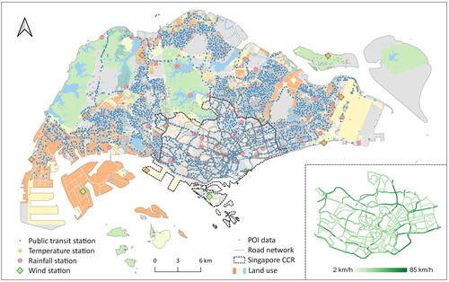
Before implementing the proposed MCGCN model, we need to collect and preprocess traffic speed and multimodal context data, respectively. Figure 3 gives an overview of the traffic speed and multimodal context datasets used in this study.

Figure 3. An overview of the traffic speed and multimodal context datasets in the study area. The subfigure provides an example of traffic speed values in Singapore’s downtown area. For simplicity, the legend for 28 kinds of land use is represented by three paralleled color-coded boxes.

4.1.1. The traffic speed dataset and preprocessing

The traffic speed dataset was collected from HERE technologies.¹ In Singapore, HERE API provides traffic speed data for each road segment. This study takes Singapore Core Central Region (CCR) as the research area, ie the downtown area of Singapore, due to the close relationship between context information and traffic flows in the downtown (Zhang and Raubal 2022). Using the API, we accessed traffic speed data (in km/h) every 2 min from 12:00pm 14 March 2022 to 12:00pm 28 March 2022, lasting for 14 days, ie two weeks. An example of traffic speed for each road segment is demonstrated in the subfigure of Figure 3. In addition, we resampled traffic speed data every 10 min by averaging all available data samples within this period to mitigate potential noise and errors. Finally, we obtained the traffic speed dataset for each road segment in Singapore CCR with a temporal resolution of 10 min.

For the road network, we used the shape information provided by the API, which contains the start point, endpoint and many intermediate points, to construct all road segments in Singapore CCR. The dataset used to construct this road network was collected on 14 March 2022. After manually removing road segments with an incorrect topology, there are a total of 1,606 available road segments.

4.1.2. The spatial context datasets and preprocessing

The spatial context influencing human mobility is diverse in the urban environment (Buchin et al. 2012). This study selects three typical types of spatial contexts from various dimensions, ie point-based POI, line-based road segments and plane-based land use. An overview of these three types of spatial contexts is shown in Figure 3. We use the road network in Section 4.1.1 as line-based road segments, which also provide their lengths and free flow speeds. The dataset details of POI and land use are as follows.

• POI: We integrated multisource POI data to generate a complete POI dataset in 2022, including Singapore OneMap,² Singapore DataMall,³ and OpenStreetMap.⁴ From OneMap, we obtained 13 classes, ie community, culture, education, emergency, employment, environment, family, government offices, health, national service, recreation, sports and others. From DataMall, we obtained one class, ie public transit stations. From OSM POI data, we obtained two classes that other sources ignore, ie commercial and hotel. From OSM building data, we extracted the center of each building as a POI point and obtained one class, ie residential. After integrating multiple sources, we attained a complete POI dataset with 17 classes containing 85,647 points in the whole of Singapore. Each POI has its category and sub-category information.

• Land use: The land use used in this study is from Singapore’s Urban Redevelopment Authority provided in 2019. After reclassifying land use types, we obtained a land use map in Singapore with 28 categories, including business, civic and community institution, commercial, educational, health and medical care, hotel, open space, park, residential, sports and recreation, transport facilities, etc. Figure 3 simplifies the legend of land use data and more details can be found at https://www.ura.gov.sg/maps/.

When using hierarchical graph learning to generate the spatial context representation of each road segment (with a distance buffer of 30 meters), we propose to include the following attribute information to model the value variations of these three spatial contexts: POIs (category and sub-category), road segments (length and free flow speed) and land use (area and category). The method of using them to generate the three-level tree has been introduced in Section 3.1.

4.1.3. The temporal context datasets and preprocessing

Compared to spatial contexts, the available temporal context data are scarce due to the limitation of temporal resolutions and simultaneity. This study employs traffic jam factors, passenger volumes of public transit stations and weather conditions as the representatives of multivariate temporal contexts.

• Traffic jam factor: The dataset was also collected through HERE API from 12:00pm 14 March 2022 to 12:00pm 28 March 2022. According to the official explanation,⁵ the jam factor is a value between 0.0 (free flow) and 10.0 (road closure) representing the expected quality of travel congestion status for each road segment. As the collection time interval is 2 min, we resampled jam factors every 10 min by averaging all available data samples within this period.

• Passenger volume: The dataset provide in-volume and out-volume passengers of each public transit station from Singapore DataMall.⁶ The public transit stations are the same POI used in the spatial context. The distribution of public transit stations is demonstrated in Figure 3, including 5,065 bus stations. For each station, DataMall furnishes tapping-in and tapping-out passenger volumes per hour by weekdays and weekends in a month. Since the traffic speed dataset is within March 2022, we employed passenger volumes in March 2022 to specify the temporal information for each road segment. Also, we assigned passenger volumes to each road segment by finding its closest public transit station. Each road segment is represented through a 96-dimensional vector to describe its temporal passenger volumes, ie 24-h workday in-volumes and out-volumes and 24-h rest-day in-volumes and out-volumes. A resampling was implemented to ensure the consistency of the temporal resolution of passenger volumes with the traffic speed dataset.

• Weather condition: Singapore provides real-time weather readings from weather stations through an open-access API.⁷ This study collected three types of weather data that may influence human mobility behaviors, ie air temperature (14 stations with a 1-min resolution), rainfall (67 stations with a 5-min resolution) and wind speed (13 stations with a 1-min resolution). The spatial distribution of weather stations is illustrated in Figure 3. For each road segment, we identified its weather conditions by finding its closest weather stations and then resampled the weather dataset into 10 min from 12:00pm 14 March 2022 to 12:00pm 28 March 2022.

4.2. Baseline models

To verify the importance of context information and compare the performance of our proposed MCGCN model with existing methods, we selected several kinds of baseline models to predict multi-step traffic speed for comparisons.

• SVR (Wei and Liu 2013): Support vector regression. As a traditional machine learning model, SVR is to process time-series data based on the support vector machine in a regression task. The experiment applies SVR with a radial basis function kernel to predict traffic speed.

• RNN (Ramakrishnan and Soni 2018): Recurrent neural network. RNN enables to capture long-term dependencies in time-series data that traditional methods fail. We utilize the bidirectional RNN with a fully connected layer by setting the hidden layer number as 5 and the hidden state size as 64.

• Seq2Seq (Karatzoglou et al. 2018): Sequence to sequence. Seq2Seq adopts the encoder-decoder framework based on gated recurrent units. The encoder produces a matching internal representation of the input, and the decoder uses this internal representation to estimate the correct output sequence in an iterative process. We set the hidden layer number as 5 and the hidden state size as 64.

• DCRNN (Li et al. 2017): Diffusion convolution recurrent neural network. DCRNN models traffic flow in the road network as a diffusion process in a directed graph. It captures spatial and temporal dependencies using bidirectional random walks and the encoder-decoder architecture with scheduled sampling, respectively. We set the diffusion step as 2, the GRU layer number as 2 and the hidden state size as 64.

• STGCN (Yu et al. 2017a): Spatial-temporal graph convolutional network. STGCN formulates the prediction problem on graphs with complete convolutional structures. Its architecture consists of several spatio-temporal convolutional blocks and an output layer. The block enables to capture spatial and temporal dependencies by combining graph convolutional layers and convolutional sequence learning layers. The number of ST-Conv blocks is set as 2 in the experiment.

• MTGNN (Wu et al. 2020): Multivariate time-series graph neural networks. MTGNN can exploit latent spatial dependencies of multivariate time-series data through graph learning and convolution. Graph learning aims to extract the directed relations among multi-variables, while the convolution module is to capture their spatial and temporal dependencies. We set the number of layers as 3 in convolution modules.

In summary, SVR belongs to the traditional machine learning method; RNN and Seq2Seq are typical models of recurrent neural networks that perform well in time-series prediction; DCRNN, STGCN and MTGNN are the state-of-the-art graph deep learning models able to capture the spatial and temporal dependencies in traffic speed forecasting.

5. Experiment and results

In this part, Section 5.1 presents the performance comparison between baseline models and the proposed MCGCN model. Following the comparison results, we analyze the effects of spatial and temporal contexts on speed prediction in Sections 5.2 and 5.3, respectively. To verify the effectiveness of our proposed modules in learning multimodal context representations, we also develop two baseline context methods to generate the corresponding baseline context representations: the baseline spatial context representations without hierarchical learning in Section 3.1.2; the baseline temporal context representations without dependency modeling in Section 3.2.2. We then utilize these context representations derived from our proposed context modules and baseline methods to predict multi-step traffic speeds and compare their performance.

5.1. Performance results

We implement the proposed MCGCN model and baseline models based on the LibCity library via Python (Wang et al. 2021). To measure and evaluate the performance of different models, mean absolute error (MAE) and root mean squared error (RMSE) are adopted as evaluation metrics. Each model is run five times, and we use the average and standard deviation of evaluation metrics to compare the performance. The experiments set the input window as 12 and the output windows as 12, which means using traffic speed in the last 12 time slots to predict traffic speed in the next 12 time slots. To be representative, we select various prediction horizons (30-min, 60-min and 120-min) that cover both short and long terms to compare the performance of different models. Except for SVR, the experiments set the epoch number as 300, and the batch size as 8, then use the Adam optimizer to guarantee the same experiment environment. The ratios of train, validation and test datasets are set as 0.7, 0.1 and 0.2, respectively. Table 1 demonstrates the average and standard deviation of evaluation metrics for multi-step traffic prediction using different models, including 30-min, 60-min and 120-min.

Table 1. The performance comparisons of multi-step traffic speed (km/h) prediction between the proposed MCGCN model and baseline models for various prediction horizons (30-min, 60-min and 120-min).

	30 min		60 min		120 min
	MAE	RMSE	MAE	RMSE	MAE	RMSE
SVR	15.03 ± 0.00	17.49 ± 0.00	15.04 ± 0.00	17.51 ± 0.00	15.07 ± 0.00	17.57 ± 0.00
RNN	5.51 ± 0.07	7.83 ± 0.09	5.51 ± 0.07	7.83 ± 0.09	5.49 ± 0.07	7.80 ± 0.09
Seq2Seq	4.26 ± 0.17	6.18 ± 0.14	4.30 ± 0.16	6.25 ± 0.13	4.52 ± 0.13	6.54 ± 0.09
DCRNN	3.83 ± 0.00	5.56 ± 0.00	3.98 ± 0.01	5.81 ± 0.01	4.22 ± 0.01	6.11 ± 0.01
STGCN	3.76 ± 0.01	5.37 ± 0.03	3.93 ± 0.03	5.65 ± 0.05	4.36 ± 0.08	6.22 ± 0.09
MTGNN	3.69 ± 0.02	5.42 ± 0.01	3.74 ± 0.02	5.54 ± 0.01	3.84 ± 0.03	5.64 ± 0.04
MCGCN	3.47 ± 0.02	4.96 ± 0.04	3.48 ± 0.02	4.96 ± 0.05	3.47 ± 0.02	4.95 ± 0.05

The row with boldface refers to the best performance in traffic forecasting.

In Table 1, the proposed MCGCN model using multimodal context information to boost traffic speed forecasting achieves the best performance compared to existing state-of-the-art models. When predicting 30-min traffic speed, the MAE and RMSE of the proposed MCGCN model achieve 3.47 ± 0.02 and 4.96 ± 0.04 km/h, respectively, which show absolute advantages over other GNN-based models in 30-min speed prediction, ie DCRNN (MAE: 3.83 ± 0.00, RMSE: 5.56 ± 0.00), STGCN (MAE: 3.76 ± 0.01, RMSE: 5.37 ± 0.03) and MTGNN (MAE: 3.69 ± 0.02, RMSE: 5.42 ± 0.01). For RNN-based models, RNN and Seq2Seq fail to capture the spatial dependency across the transportation network, leading to dissatisfactory outcomes in 30-min speed prediction with the MAE of 5.51 ± 0.07 and 4.26 ± 0.17 km/h, respectively. As a traditional method, SVR performs the worst due to its limitations in modeling the non-linear relationship and the long-term dependency.

In long-term traffic speed forecasting, we find the proposed MCGCN model is also superior compared to other baseline models in Table 1. In 60-min speed prediction, the MAE of MCGCN using context information is 3.48 ± 0.02 km/h, with an average MAE improvement of 0.50, 0.45 and 0.26 km/h compared to DCRNN, STGCN and MTGNN, respectively. This comparison also achieves a good performance in 120-min speed prediction, ie with an average MAE improvement of 0.75, 0.89 and 0.37 km/h for DCRNN, STGCN and MTGNN, respectively. Focusing on the change of evaluation metrics from 30-min to 120-min speed prediction, most models are in an increasing trend due to error accumulation, such as Seq2Seq, DCRNN, STGCN and MTGNN. However, this error accumulation can be mitigated in our proposed MCGCN model.⁸ After integrating multimodal context information into traffic speed prediction, the MCGCN model can exploit spatial and temporal context information provided by surrounding environments to achieve good performance in long-term speed prediction. For example, POIs enable the model to distinguish road segments with different levels of attractiveness to vehicles from a spatial perspective; traffic jam factors can benefit long-term speed prediction by considering the traffic congestion status of each road segment from a temporal perspective. Generally, multimodal context information takes great effects on traffic speed prediction, especially long-term speed prediction.

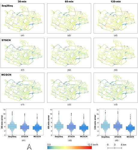
Furthermore, Figure 4 demonstrates the spatial distribution of prediction errors between the predicted speed and the observed speed for each road segment. We visualize 30-min, 60-min and 120-min prediction error maps and boxen plots with three representative models, ie Seq2Seq (RNN-based model), STGCN (GNN-based model) and MCGCN (context-based model). From a vertical view of Figure 4, the prediction error ranges of these three models differ a lot, with Seq2Seq performing the worst and MCGCN performing the best shown in Figure 4(d1–d3). For Seq2Seq, several road segments in red hold high prediction errors compared to their neighboring road segments in Figure 4(a1–a3). This problem gets solved when using STGCN and MCGCN to predict speed, especially for 30-min STGCN prediction in Figure 4(b1) and all MCGCN-based prediction in Figure 4(c1–c3). Essentially, Seq2Seq fails to capture spatial dependencies of traffic speed information in the road network, while STGCN can take advantage of the neighboring information of each road segment to reduce prediction errors. For MCGCN, it outperforms the above-mentioned two models in reducing high prediction errors of particular road segments by exploiting situation-dependent information. From a horizontal view of Figure 4, the prediction error maps of Seq2Seq and STGCN present an apparent increase from Figure 4(a1) to (a3) and from Figure 4(b1) to (b3), respectively, revealing the error accumulation process in multi-step traffic speed prediction. This accumulation is consistent with their MAE and RMSE values in Table 1. In contrast, the proposed MCGCN model performs well in multi-step traffic speed prediction, with little accumulation of prediction errors from Figure 4(c1) to (c3), which can also be observed from Figure 4(d1) to (d3). This phenomenon further emphasizes the importance of context information in long-term traffic speed prediction by mitigating prediction errors and improving performance.

Figure 4. Prediction error maps of road segments between the predicted speed and the observed speed for various prediction horizons (30-min, 60-min and 120-min) with three representative models. (a1–a3) Seq2Seq. (b1–b3) STGCN. (c1–c3) The proposed MCGCN model. (d1–d3) Boxen plots of the above three models to illustrate their error distribution of 30-min, 60-min and 120-min speed prediction. The columns from left to right represent different horizons, ie 30-min, 60-min and 120-min. The color bar below shows the prediction error range for a1–c3.

5.2. Spatial context embedding and analysis

The spatial context exerts influence on human mobility by simultaneously enabling and limiting individual movement in the urban space (Buchin et al. 2012). To quantify the influence, we organize the spatial context data from various dimensions, namely, zero-dimensional POIs, one-dimensional road segments and two-dimensional land use, into a three-level tree. Then, we employ the proposed spatial embedding method in Section 3.1.2 to learn the spatial context representation of each tree in a hierarchical manner, which can encode the local and global structural information in the built tree. To evaluate the effectiveness of this hierarchical method, its performance on representation learning and speed prediction is compared with a baseline method without hierarchical learning. We leverage the traffic congestion status of each road segment to supervise the learning process of spatial context representations. This traffic congestion status is extracted from averaging traffic jam factors of each road segment per 10 min during the period.

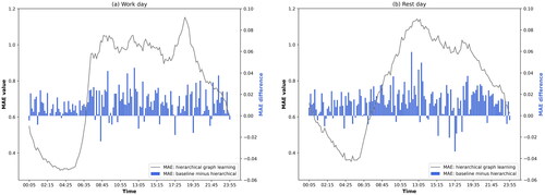
Figure 5 illustrates MAE values of learning spatial context representations using the hierarchical method and their differences from the non-hierarchical baseline method. When the MAE difference is above zero, the hierarchical method performs better than the non-hierarchical one and vice versa. First, we found that the overall tendency of MAE curves exhibits similar patterns to human traveling behaviors, ie high values distributed over morning and afternoon peak hours due to residents’ commuting activities during work days, and high values distributed over noon hours due to residents’ entertainment activities during rest days (Tu et al. 2017). According to the MAE difference between the two methods, we found that hierarchical learning performs better than the non-hierarchical baseline method in most of the time slots for both work and rest days. Among 144 time slots, there are only 18 workday time slots in Figure 5(a) and 23 rest-day time slots in Figure 5(b) that the non-hierarchical method has lower MAE values. This phenomenon implies that the hierarchical learning method can better model spatial contexts to understand the patterns of traffic congestion status.

Figure 5. MAE values of learning the spatial context representations using the proposed hierarchical learning method and their differences from the non-hierarchical method every 10 min (ie non-hierarchical MAE – hierarchical MAE). (a) Workday. (b) Rest day.

To further test the performance of hierarchical learning, we employ the spatial context representations generated by the hierarchical and non-hierarchical methods to predict traffic speed, respectively. Table 2 demonstrates the results of 30-min, 60-min and 120-min speed prediction using these two methods, which can verify the advantage of hierarchical learning. In 30-min speed prediction, the hierarchical and non-hierarchical methods hold the same performance with an average MAE of 3.74 ± 0.01 km/h. However, the hierarchical method performs better than the non-hierarchical method in 60-min and 120-min speed prediction, with an average MAE improvement of 0.02 and 0.13 km/h, respectively. This outcome reveals the superiority of the proposed hierarchical method in learning spatial context representations, which can benefit long-term speed prediction more than the non-hierarchical model. Using the hierarchical method also leads to more stable performance in traffic speed forecasting. The standard deviation of MAE for multi-step prediction maintains lower values than those of the non-hierarchical method, especially for 120-min speed prediction.

Table 2. The performance of multi-step traffic speed prediction for various prediction horizons (30-min, 60-min and 120-min; km/h) using the hierarchical and non-hierarchical methods to learn spatial context representations.

	30 min		60 min		120 min
	MAE	RMSE	MAE	RMSE	MAE	RMSE
No hierarchy	3.74 ± 0.01	5.35 ± 0.01	3.85 ± 0.03	5.54 ± 0.04	4.04 ± 0.13	5.82 ± 0.15
With hierarchy	3.74 ± 0.01	5.35 ± 0.01	3.83 ± 0.02	5.52 ± 0.02	3.91 ± 0.02	5.66 ± 0.03

5.3. Temporal context modeling and analysis

Multivariate time-series techniques play a crucial role in exploiting latent dependencies of multiple temporal contexts and improving the performance of time-series prediction (Cao et al. 2020). However, previous research ignores the dependencies hidden in multivariate temporal contexts and their influences on traffic speed prediction. This study proposes a temporal context modeling module in Section 3.2 to overcome this problem by constructing subgraphs that associate multivariate temporal contexts over different road segments. To justify the effects of the proposed method on learning temporal context representations, we compare its performance in context-based traffic speed prediction with a baseline method that also learns temporal context representations without dependency modeling.

Table 3 displays the performance of traffic speed prediction using the temporal context representations learned by two methods, ie the dependency and non-dependency methods. An important phenomenon is that the error accumulation process can be mitigated using both two methods, without obvious MAE and RMSE increases from 30-min to 120-min speed prediction. In detail, the MAE values using the non-dependency method are within the range of 3.52–3.55 km/h, while the MAE value for three prediction horizons using the dependency method is 3.50 ± 0.02 km/h. This phenomenon suggests that long-term speed prediction can be greatly improved by temporal contexts regardless of the method used to learn their representations. The other important observation is that the dependency method consistently outperforms the non-dependency method across all prediction horizons. The MAE values of the dependency method are lower than the corresponding values of the non-dependency method for each prediction horizon, with an improvement of 0.02, 0.05 and 0.04 km/h. This outcome reveals that the proposed temporal context modeling module can better advance the performance of traffic speed prediction by capturing latent dependencies of multivariate temporal contexts.

Table 3. The performance of multi-step traffic speed prediction for various prediction horizons (30-min, 60-min and 120-min; km/h) using the dependency and non-dependency methods to learn temporal context representations.

	30 min		60 min		120 min
	MAE	RMSE	MAE	RMSE	MAE	RMSE
No dependency	3.52 ± 0.02	5.05 ± 0.04	3.55 ± 0.02	5.08 ± 0.04	3.54 ± 0.01	5.06 ± 0.03
With dependency	3.50 ± 0.02	5.03 ± 0.04	3.50 ± 0.02	5.04 ± 0.04	3.50 ± 0.02	5.03 ± 0.03

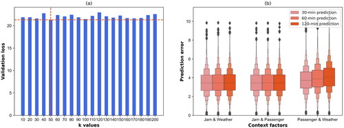
When using the proposed dependency method to learn temporal context representations, a crucial parameter is to identify a suitable subgraph size that balances the ability to model dependencies and computation cost. Figure 6(a) illustrates the validation loss of multi-step traffic speed prediction using different subgraph sizes, eg k mentioned in Section 3.2. The validation loss achieves the lowest value when the subgraph size is 50. Therefore, we utilize k = 50 for all the experiments in this study when modeling the dependencies of multivariate temporal contexts. After identifying the suitable subgraph size, one question arises of how different combinations of multivariate temporal contexts affect traffic speed prediction. As shown in Figure 6(b), we observe that the jam factor occupies the dominant position compared to passenger volumes and weather conditions. For the first two combinations involving jam factors, their boxen plots of prediction errors for various prediction horizons are all obviously lower than the third combination (without using jam factors). In addition, the error accumulation process from 30-min to 120-min prediction is not obvious for the first two combinations, while the third combination presents an evident increase of prediction errors. Essentially, the jam factor reflects the traffic congestion status of each road segment, which can significantly improve the predicted speed variations in the subsequent time slots. However, passenger volumes are more likely regarded as a time proxy indicating the morning and afternoon peak hours of urban residents’ commute on work and rest days. Thus, this dataset is not intended to impact road speeds directly but to imply the association with fluctuations in public transit usage over time. As to weather data, it can also greatly boost traffic speed prediction under different meteorological conditions, but its benefits are limited in daily speed prediction.

Figure 6. Performance analysis of multivariate temporal context modeling using different subgraph sizes and temporal context variables. (a) Validation loss of speed prediction when modeling multivariate temporal contexts with various subgraph sizes, ie k. (b) Prediction errors of speed prediction when using three different combinations of temporal contexts, ie (1) jam factors and weather conditions, (2) jam factors and passenger volumes and (3) passenger volumes and weather conditions.

6. Conclusion

Context information plays a vital role in understanding human mobility patterns and boosting traffic forecasting (Sharif and Alesheikh 2017, Tedjopurnomo et al. 2020). However, the diversity and modalities of context information hinder utilizing it to advance traffic forecasting. To solve this problem, this study proposed a multimodal context-based graph convolutional neural network (MCGCN) model to incorporate different context information into traffic speed forecasting, which achieved state-of-the-art performance compared to baseline models. For the spatial context, we utilized a hierarchical spatial embedding module to generate representations by organizing spatial context data from different dimensions, which outperforms the non-hierarchical method in modeling spatial contexts. The experiment verified its effectiveness in traffic speed forecasting. For the temporal context, we designed a multivariate temporal modeling module to capture latent dependencies of temporal context data and produce representations for traffic speed forecasting. We also found that the jam factor can dominantly affect the prediction performance compared to other temporal contexts. Finally, we employed an attention-based multimodal fusion layer to integrate traffic speed with the spatial and temporal context representations for traffic speed forecasting. The outcomes justify the feasibility of the proposed MCGCN model and demonstrate the significant role of context information in GeoAI research.

So far, traffic congestion has substantially impacted social capital and environmental protection for urban areas worldwide. Based on our model’s obtained speed prediction results, stakeholders can acquire accurate traffic speed information and understand what factors most affect the prediction performance. Also, there are some other potential applications, such as improving traffic signal optimization to reduce congestion and assist in dynamic route planning for individual drivers, public transportation and emergency services. Overall, urban planners can better manage the urban transportation system to decrease the adverse influence of traffic congestion on economic activities. On the other hand, the proposed MCGCN model can potentially attract GIS researchers to pay more attention to context information ubiquitously distributed over the urban environment, which can benefit downstream applications. This study proposes to divide context information into two types, ie spatial and temporal contexts, and accordingly developed two embedding modules to capture their characteristics. This division and the proposed modules can also be transferred to other GIS studies when context information takes effect on their research, such as land use modeling and population distribution mapping. In detail, land use recognition can utilize the hierarchical spatial embedding module to generate more comprehensive spatial representations that consider its surrounding environment to classify land use, while population distribution mapping can benefit from the multivariate temporal modeling module to capture dynamic information of passenger volumes in nearby public transit stations.

However, this study still encounters several unsolved problems. First, we ignored the correlated information of context data amongst multiple modalities, ie cross-modality relations, which can help better fuse multimodal context data from various sources. Second, although this study investigated how different contexts affect traffic speed forecasting, the causal relationship is still unclear due to the lack of explainability of deep learning models, which deserves further exploration. Third, although we considered several representative contextual factors as the input for traffic speed forecasting, these factors are still a small part of all kinds of context information due to their ubiquitous distribution over the urban environment. For example, temporal contexts contain more than the time-varying variables mentioned in this study. They also include features associated with hourly, weekly, or other factors related to duration or time of day, all of which fall within the realm of temporal contexts and deserve further investigation in traffic forecasting (Tedjopurnomo et al. 2020). In practice, incorporating additional contexts into the MCGCN model is feasible and potentially beneficial for improving its predictive power, but each additional context comes with its own challenges, eg data completeness, availability and reliability. Nevertheless, these challenges can be managed with appropriate data processing and feature embedding. Meanwhile, weather data have influential effects on traffic speed forecasting under various weather conditions (Ryu et al. 2020), but this study is mainly focused on daily traffic speed prediction, limiting its ability to improve prediction accuracy. Finally, while this study evaluates the MCGCN model’s predictive performance within a 2-h window, a technical expansion of this prediction window, for instance, to 10 h, is feasible. However, such a substantial extension in the prediction horizon may introduce complexities in preserving the existing level of prediction error, considering the vast array of unpredictable factors that can influence traffic conditions. In future studies, we will include more context datasets and research how to effectively integrate them into context-aware traffic studies.

Acknowledgments

The research was conducted at the Future Resilient Systems program at the Singapore-ETH Centre, which was established collaboratively between ETH Zurich and the National Research Foundation Singapore.

Disclosure statement

No potential conflict of interest was reported by the author(s).

Data and codes availability statement

The data and codes supporting the main findings of this study are available at https://doi.org/10.6084/m9.figshare.21813048.v1.

Additional information

Funding

This research is supported by the National Research Foundation Singapore (NRF) under its Campus for Research Excellence and Technological Enterprise (CREATE) program.

Notes on contributors

Yatao Zhang

Yatao Zhang is a doctoral student at the Mobility Information Engineering lab at ETH Zurich and the Future Resilient Systems at the Singapore-ETH Center. His research interests lie in context-based spatiotemporal analysis, geospatial big data mining and traffic forecasting.

Tianhong Zhao

Tianhong Zhao is a lecturer at the College of Big Data and Internet, Shenzhen Technology University. He received his PhD degree from Shenzhen University in 2023. His research interests include graph neural networks and spatiotemporal big data analysis.

Song Gao

Song Gao is an associate professor in GIScience at the Department of Geography, University of Wisconsin-Madison. He holds a PhD in Geography at the University of California, Santa Barbara. His main research interests include place-based GIS, geospatial data science and GeoAI approaches to human mobility and social sensing.

Martin Raubal

Martin Raubal is a professor of geoinformation engineering at ETH Zurich. His research interests focus on spatial decision-making for sustainability, more specifically he concentrates on analyzing spatio-temporal aspects of human mobility, spatial cognitive engineering and mobile eye-tracking to investigate visual attention while interacting with geoinformation and in spatial decision situations.

Notes

1 See https://www.here.com/.

2 An authoritative national map of Singapore with the most detailed and timely updated information developed by the Singapore Land Authority. See https://www.onemap.gov.sg/.

3 A wide variety of land transport-related datasets provided by the Singapore Land Authority. See https://datamall.lta.gov.sg/content/datamall/en.html.

4 An open-source crowdsourcing data platform. See https://www.openstreetmap.org/.

5 See https://developer.here.com/documentation/traffic/dev_guide/topics/common-acronyms.html.

6 See https://datamall.lta.gov.sg/content/datamall/en/dynamic-data.html.

7 See https://data.gov.sg/dataset/realtime-weather-readings.

8 The error accumulation still exists in our proposed MCGCN model. Its MAE value in 10-min speed prediction is 3.13 ± 0.02 km/h, which increases to 3.44 ± 0.02 and 3.47 ± 0.02 km/h in 20-min and 30-min speed prediction, respectively.

References

- Azad, A. and Wang, X., 2021. Land use change ontology and traffic prediction through recurrent neural networks: a case study in Calgary, Canada. ISPRS International Journal of Geo-Information, 10 (6), 358.
- Belhadi, A., et al., 2020. A recurrent neural network for urban long-term traffic flow forecasting. Applied Intelligence, 50 (10), 3252–3265.
- Buchin, M., Dodge, S., and Speckmann, B., 2012. Context-aware similarity of trajectories. In: International conference on geographic information science, Columbus, OH, USA. Berlin, Heidelberg: Springer, 43–56.
- Cao, D., et al., 2020. Spectral temporal graph neural network for multivariate time-series forecasting. Advances in Neural Information Processing Systems, 33, 17766–17778.
- Chen, J., et al., 2020. Gst-gcn: a geographic-semantic-temporal graph convolutional network for context-aware traffic flow prediction on graph sequences. In: 2020 IEEE international conference on systems, man, and cybernetics (SMC), Toronto, ON, Canada. IEEE, 1604–1609.
- Cheng, A., et al., 2017. Multiple sources and multiple measures based traffic flow prediction using the chaos theory and support vector regression method. Physica A: Statistical Mechanics and Its Applications, 466, 422–434.
- Demšar, U., et al., 2021. Establishing the integrated science of movement: bringing together concepts and methods from animal and human movement analysis. International Journal of Geographical Information Science, 35 (7), 1273–1308.
- Diao, Z., et al., 2019. Dynamic spatial-temporal graph convolutional neural networks for traffic forecasting. Proceedings of the AAAI Conference on Artificial Intelligence, 33 (1), 890–897.
- Ermagun, A. and Levinson, D., 2018. Spatiotemporal traffic forecasting: review and proposed directions. Transport Reviews, 38 (6), 786–814.
- Fu, R., Zhang, Z., and Li, L., 2016. Using LSTM and GRU neural network methods for traffic flow prediction. In: 2016 31st youth academic annual conference of Chinese Association of Automation (YAC), Wuhan, China. IEEE, 324–328.
- Gao, J., et al., 2020. A survey on deep learning for multimodal data fusion. Neural Computation, 32 (5), 829–864.
- Ge, L., et al., 2019a. Temporal graph convolutional networks for traffic speed prediction considering external factors. In: 2019 20th IEEE international conference on mobile data management (MDM), Hong Kong, China. IEEE, 234–242.
- Ge, Y., et al., 2019b. Principles and methods of scaling geospatial earth science data. Earth-Science Reviews, 197, 102897.
- Guo, D., et al., 2022. Deepssn: a deep convolutional neural network to assess spatial scene similarity. Transactions in GIS, 26 (4), 1914–1938.
- Han, C. and Song, S., 2003. A review of some main models for traffic flow forecasting. In: Proceedings of the 2003 IEEE international conference on intelligent transportation systems, Shanghai, China. IEEE, 216–219.
- Haraguchi, M., et al., 2022. Human mobility data and analysis for urban resilience: a systematic review. Environment and Planning B: Urban Analytics and City Science, 49 (5), 1507–1535.
- He, K., et al., 2015. Spatial pyramid pooling in deep convolutional networks for visual recognition. IEEE Transactions on Pattern Analysis and Machine Intelligence, 37 (9), 1904–1916.
- Huang, Q. and Wong, D.W., 2015. Modeling and visualizing regular human mobility patterns with uncertainty: an example using twitter data. Annals of the Association of American Geographers, 105 (6), 1179–1197.
- Janowicz, K., et al., 2020. GeoAI: spatially explicit artificial intelligence techniques for geographic knowledge discovery and beyond. International Journal of Geographical Information Science, 34 (4), 625–636.
- Jiang, W. and Luo, J., 2022. Graph neural network for traffic forecasting: a survey. Expert Systems with Applications, 207, 117921.
- Karatzoglou, A., Jablonski, A., and Beigl, M., 2018. A seq2seq learning approach for modeling semantic trajectories and predicting the next location. In: Proceedings of the 26th ACM SIGSPATIAL international conference on advances in geographic information systems, Seattle, WA, USA. Association for Computing Machinery, 528–531,
- Kashyap, A.A., et al., 2022. Traffic flow prediction models–a review of deep learning techniques. Cogent Engineering, 9 (1), 2010510.
- Koesdwiady, A., Soua, R., and Karray, F., 2016. Improving traffic flow prediction with weather information in connected cars: a deep learning approach. IEEE Transactions on Vehicular Technology, 65 (12), 9508–9517.
- Kumar, N. and Raubal, M., 2021. Applications of deep learning in congestion detection, prediction and alleviation: a survey. Transportation Research Part C: Emerging Technologies, 133, 103432.
- Kurth, M., et al., 2020. Lack of resilience in transportation networks: economic implications. Transportation Research Part D: Transport and Environment, 86, 102419.
- Lahat, D., Adali, T., and Jutten, C., 2015. Multimodal data fusion: an overview of methods, challenges, and prospects. Proceedings of the IEEE, 103(9), 1449–1477.
- Lana, I., et al., 2018. Road traffic forecasting: recent advances and new challenges. IEEE Intelligent Transportation Systems Magazine, 10 (2), 93–109.
- Lee, M. and Holme, P., 2015. Relating land use and human intra-city mobility. PLoS One, 10 (10), e0140152.
- Li, M. and Zhu, Z., 2021. Spatial-temporal fusion graph neural networks for traffic flow forecasting. In: Proceedings of the AAAI conference on artificial intelligence. 35 (5), 4189–4196.
- Li, S., et al., 2016. Geospatial big data handling theory and methods: a review and research challenges. ISPRS Journal of Photogrammetry and Remote Sensing, 115, 119–133.
- Li, Y. and Shahabi, C., 2018. A brief overview of machine learning methods for short-term traffic forecasting and future directions. Sigspatial Special, 10 (1), 3–9.
- Li, Y., et al., 2017. Diffusion convolutional recurrent neural network: data-driven traffic forecasting. arXiv preprint arXiv:1707.01926.
- Lin, L., et al., 2018. Road traffic speed prediction: a probabilistic model fusing multi-source data. IEEE Transactions on Knowledge and Data Engineering, 30 (7), 1310–1323.
- Liu, J., et al., 2020. Urban big data fusion based on deep learning: an overview. Information Fusion, 53, 123–133.
- Liu, K., et al., 2018. Learn to combine modalities in multimodal deep learning. arXiv preprint arXiv:1805.11730.
- Liu, Y. and Wu, H., 2017. Prediction of road traffic congestion based on random forest. In: 2017 10th international symposium on computational intelligence and design (ISCID), Hangzhou, China. IEEE, 361–364.
- Liu, Y., et al., 2017. Short-term traffic flow prediction with conv-LSTM. In: 2017 9th international conference on wireless communications and signal processing (WCSP), Nanjing, China. IEEE, 1–6.
- Ramakrishnan, N. and Soni, T., 2018. Network traffic prediction using recurrent neural networks. In: 2018 17th IEEE international conference on machine learning and applications (ICMLA), Orlando, FL, USA. IEEE, 187–193.
- Ren, Y., et al., 2020. A hybrid integrated deep learning model for the prediction of citywide spatio-temporal flow volumes. International Journal of Geographical Information Science, 34 (4), 802–823.
- Ryu, S., Kim, D., and Kim, J., 2020. Weather-aware long-range traffic forecast using multi-module deep neural network. Applied Sciences, 10 (6), 1938.
- Sattar, F., et al., 2016. Recent advances on context-awareness and data/information fusion in its. International Journal of Intelligent Transportation Systems Research, 14 (1), 1–19.
- Sharif, M. and Alesheikh, A.A., 2017. Context-awareness in similarity measures and pattern discoveries of trajectories: a context-based dynamic time warping method. GIScience & Remote Sensing, 54 (3), 426–452.
- Tedjopurnomo, D.A., et al., 2020. A survey on modern deep neural network for traffic prediction: trends, methods and challenges. IEEE Transactions on Knowledge and Data Engineering, 34 (4), 1544–1561.
- Tu, W., et al., 2017. Coupling mobile phone and social media data: a new approach to understanding urban functions and diurnal patterns. International Journal of Geographical Information Science, 31 (12), 2331–2358.
- Tu, W., et al., 2020a. Scale effect on fusing remote sensing and human sensing to portray urban functions. IEEE Geoscience and Remote Sensing Letters, 18 (1), 38–42.
- Tu, W., et al., 2020b. Portraying the spatial dynamics of urban vibrancy using multisource urban big data. Computers, Environment and Urban Systems, 80, 101428.
- Wang, H.-W., et al., 2020. Evaluation and prediction of transportation resilience under extreme weather events: a diffusion graph convolutional approach. Transportation Research Part C: Emerging Technologies, 115, 102619.
- Wang, J., et al., 2021. Libcity: an open library for traffic prediction. In: Proceedings of the 29th international conference on advances in geographic information systems, Beijing, China. Association for Computing Machinery, 145–148.
- Wang, S., et al., 2018. A context-based geoprocessing framework for optimizing meetup location of multiple moving objects along road networks. International Journal of Geographical Information Science, 32 (7), 1368–1390.
- Wei, D. and Liu, H., 2013. An adaptive-margin support vector regression for short-term traffic flow forecast. Journal of Intelligent Transportation Systems, 17 (4), 317–327.
- Wu, Y., et al., 2018. A hybrid deep learning based traffic flow prediction method and its understanding. Transportation Research Part C: Emerging Technologies, 90, 166–180.
- Wu, Z., et al., 2020. Connecting the dots: multivariate time series forecasting with graph neural networks. In: Proceedings of the 26th ACM SIGKDD international conference on knowledge discovery & data mining, Virtual Event, CA, USA. Association for Computing Machinery, 753–763.
- Yin, X., et al., 2022. Deep learning on traffic prediction: methods, analysis and future directions. IEEE Transactions on Intelligent Transportation Systems, 23 (6), 4927–4943.
- Yin, Y. and Shang, P., 2016. Forecasting traffic time series with multivariate predicting method. Applied Mathematics and Computation, 291, 266–278.
- Ying, Z., et al., 2018. Hierarchical graph representation learning with differentiable pooling. Advances in Neural Information Processing Systems, 31.
- Yu, B., Yin, H., and Zhu, Z., 2017a. Spatio-temporal graph convolutional networks: a deep learning framework for traffic forecasting. arXiv preprint arXiv:1709.04875.
- Yu, R., et al., 2017b. Deep learning: a generic approach for extreme condition traffic forecasting. In: N. Chawla and W. Wang, eds. Proceedings of the 2017 SIAM international conference on data mining. Society for Industrial and Applied Mathematics, 777–785.
- Zhang, Y. and Raubal, M., 2022. Street-level traffic flow and context sensing analysis through semantic integration of multisource geospatial data. Transactions in GIS, 26 (8), 3330–3348.
- Zhao, P., et al., 2020. Where to go next: a spatio-temporal gated network for next poi recommendation. IEEE Transactions on Knowledge and Data Engineering, 34(5), 2512–2524.
- Zhao, T., et al., 2022. Coupling graph deep learning and spatial-temporal influence of built environment for short-term bus travel demand prediction. Computers, Environment and Urban Systems, 94, 101776.