A raster-based method for the hierarchical selection of river networks based on stream characteristics

Abstract

Computer screens often constrain the level of detail and clarity of displays. High-density data require a predefined strategy to select significant features hierarchically to allow interactive data zooming. Although many methods are available for hierarchically selecting rivers from vector data, some approaches for raster data are better than others for maintaining accuracy when the original river data are in a raster format during generalization. In this study, a raster-based approach is proposed to allow hierarchical superpixel selection in river networks. Linear spectral clustering segmentation was applied to divide the original raster river networks into superpixels at multiple levels. A graph was constructed to organize the generated river network superpixels based on the distances between adjacent superpixels by considering the weights determined by the four types of rules. Finally, the total weight values were ranked, the river-network superpixels were selected according to their weights, and the redundant pixels at the river-network intersections were removed. Compared with the traditional vector selection method, the proposed superpixel river network selection method can effectively consider the characteristics of river width without artificial river grading and preserve the main structure and connectivity features during hierarchical mapping. Notably, the average geometry and density changes decreased by 15.8% and 5.1%, respectively.

Keywords:

• River selection
• superpixel segmentation
• raster data
• map generalization

1. Introduction

Because the Earth is rich in multiple types of water resources, different topographical structures result in the formation of many intersecting river networks with various forms (Herzog et al. 2019, Durighetto et al. 2020). As the display scale decreases, the information load for a fixed screen area becomes limited, which may lead to highly dense river networks exhibiting considerable crowding. To avoid the cognitive burden of crowding and allow the efficient extraction of the main information from several river networks, such as overall distribution characteristics, a selection operation for hierarchical mapping is usually applied (Chen et al. 2009, Li and Zhou 2012, Han et al. 2020). In river network selection, the secondary branches are removed and the main rivers with satisfactory overall characteristics, including relative distribution, stream density, and local characteristics, (including the longest branches) are preserved (Ai et al. 2009, Yang and Li 2012, Huang et al. 2017).

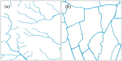
The traditional selection methods for linear features in network structures have two limitations. First, when the map data source is in a raster format, such as for remote sensing images and binary images, many raster-based generalization methods are widely used (Schylberg 1993, Li 1994, Shen et al. 2022). For example, Shen et al. (2022) used deep learning and raster-based generalization algorithms for the multiscale representation of urban buildings on the basis of hyperspectral remote sensing images. However, the existing vector-based selection methods cannot directly handle river networks in raster format, unless the vector data are converted to raster data. This data conversion process can lead to the loss of map information and accuracy and may require additional algorithms or software support. Second, traditional vector-based methods for river network selection are usually designed primarily for river networks without a mesh structure, such as the natural river network (Figure 1(a)). In these methods, many characteristics of river networks, including the drainage area (Ai et al. 2006) and river length, level, and width (Horton 1945, Strahler 1952), are considered. However, in actual situations, river networks typically contain many mesh structures as shown in the urban river network in Figure 1(b). Selection methods for river networks with mesh structures based on traditional strategies using vector-based methods remain challenging because the connectivity characteristics of the river network structure are usually not considered.

Figure 1. River networks with and without mesh structures (a) Natural river network without a mesh structure (b) Urban river network with a mesh structure.

In this study, to address these two limitations, we developed a raster-based selection method for polygonal river networks in a standard image format that can automatically identify grading information by combining superpixel segmentation and graph technologies.

The rest of this study is organized as follows: Section 2 describes the work related to selecting linear features involving network structures, including vector-based road and river selection methods. Section 3 describes the methods used to allow the selection of river networks, considering multiple feature constraints, which include the following three main steps: hierarchical superpixel segmentation using the linear spectral clustering (LSC) method, the weighting of the river network superpixels based on the graph structure, and the generation of the selection results by implementing total weight ranking and removing redundant pixels at intersections. Section 4 describes the process of considering the river network in Guangdong Province, China, to perform selection operations. The original experimental data, implementation processes, and results of the comparisons of the proposed approach with traditional vector-based methods are also discussed. Section 5 includes concluding remarks and describes the study’s limitations and future scopes.

2. Related work

2.1. River selection methods

Many existing road selection methods have been proposed for the selection of linear features on a map, which can be divided into the following five main types: semantics-based methods (Jiang and Claramunt 2004), mesh-based methods (Chen et al. 2009), stroke-based methods (Edwardes and Mackaness 2000, Heinzle et al. 2005, Yang et al. 2011, Li and Zhou 2012), graph-based methods (Mackaness and Beard 1993, Mackaness 1995, Jiang and Claramunt 2004), and mixed technology methods (Brewer et al. 2013, Zhou and LI 2016, Shoman and Gulgen 2017, Han et al. 2020). Even though these road selection methods can consider the relevant attributes and topological, structural, distribution, geometry, connectivity, and contextual characteristics, they cannot be applied to raster data. Generally, river selection methods have garnered less attention compared with road network selection methods because river networks exhibit typical grading and varying width characteristics, which make their processing difficult. In the existing river selection methods (Ai et al. 2006, Touya 2007, Ai et al. 2009, Stanislawski 2009, Buttenfield et al. 2011, Yang and Li 2012, Touya & Girres 2013, Huang et al. 2017, Stum et al. 2017, McManamay and DeRolph 2019, Li et al. 2020), researchers did not consider the varying width characteristics of rivers. For example, Ai et al. (2009) reported a method for river network generalization on the basis of watershed divisions and tree structures. Through this method, river networks at different levels of detail can be selected and ordered according to practical requirements. Yang and Li (2012) reported a method for river vector selection that considers the importance of branches and intersection points. This method can effectively maintain the original river structure. Huang et al. (2017) reported a matrix-based method for the variable-scale vector representation of river networks based on pruning and simplification operations. Usually, matrix-based methods can outperform traditional methods. Li et al. (2020) reported a method for selecting river networks with dendritic patterns using hybrid coding. In this method, the river networks were divided into the following three types of branches: deep, shallow, and moderate. Furthermore, Horton coding is used to code and automatically select the original dendritic river network, and the selection results can effectively highlight hierarchies and maintain the distribution characteristics of the tributaries.

However, in the abovementioned methods, because the original varying width and mesh characteristics of rivers are not considered during selection, inaccurate results may be obtained because the width information considerably affects the identification of the main river channels and tributaries.

2.2. Superpixel segmentation methods

Superpixels consist of adjacent normal pixel groups with similar colors, intensities, textures, or other features (Bergh et al. 2012, Shen et al. 2019). Many algorithms have been developed to generate superpixels (Yu and Shi 2003, Moore et al. 2008, Levinshtein et al. 2009, Veksler et al. 2010, Liu et al. 2011, Achanta et al. 2012, Bergh et al. 2012, Li and Chen 2015), and each superpixel algorithm has their own specific advantages. For example, Achanta et al. (2012) reported a simple linear iterative clustering (SLIC) method based on k-means clustering. In this method, weighted color and spatial distances were used to measure the similarity of pixels. The SLIC method exhibited high temporal efficiency. Levinshtein et al. (2009) reported a special method to generate superpixels with high densities, which effectively enhanced the compactness of the generated superpixels. To address the issue that most superpixel algorithms generate irregular pixel paths, Veksler et al. (2010) used an energy function to produce superpixels with highly regular shapes. This method had high temporal efficiency and satisfactory boundary recall. Furthermore, in the LSC method (Li and Chen 2015), a kernel function is used rather than traditional eigenbased algorithms to estimate the similarity measure, resulting in the explicit mapping of pixel values and coordinates to a higher-dimensional feature space. The key objective in LSC involves explicitly utilizing the relationship between the weighted k-mean optimization objective and the selected normalized result by introducing a well-designed high-dimensional space (Li and Chen 2015). This approach can effectively maintain the original boundaries of the segmented objects. More details on the LSC method can be found in the reference (Li and Chen 2015). Although the superpixel segmentation technique is used for the simplification (Shen et al. 2018) and aggregation (Shen et al. 2019) of objects during map generalization, it has not been used for selecting river networks.

Considering the work related to selecting linear features, the limitations of the existing methods are as follows:

1. Traditional river network selection methods are designed only for rivers without mesh structures; therefore, these methods cannot fulfill practical requirements because river networks, such as urban water networks, often have a mesh structure.

2. Traditional methods consider the drainage area and river length, width, and level among other characteristics. However, during river network selection, the connectivity of a river network with a mesh structure is not guaranteed.

Because these methods for selecting linear features on the basis of vectors are relatively abundant, in this study, we addressed the abovementioned gaps by combining superpixel segmentation and graph technologies. The river width and the global structure and the local connectivity characteristics of river networks were considered during the selection.

3. Methodology for the selection of raster river networks

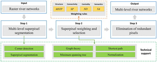
As shown in Figure 2, the proposed superpixel river network selection (SRNS) method for selecting raster river networks can be divided into the following three steps: the multilevel superpixel segmentation of raster river networks, the implementation of river network superpixel weighting, and the selection and elimination of redundant pixels at river network intersections.

Figure 2. The selection of raster river networks.

3.1. Multilevel superpixel segmentation of raster river networks

To select river networks, we first divide raster river networks into superpixels, which are the basic operational units in the selection process. In this study, the LSC approach, which showed outstanding performance in preserving the original boundaries of segmented objects (Li and Chen 2015), was applied to multilevel superpixel segmentation of raster river networks. The adopted approach involves the following four steps.

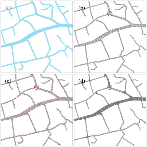
1. Preliminary division of the raster river networks using the LSC superpixel segmentation method. The original discrete pixels that form a river network can be clustered into pixel blocks within a certain distance. Figure 3(a) shows a PNG image of a river network transformed from a vector polygonal format with an original scale of 1:25000 using ArcGIS software (ESRI, USA), with a pixel size of $2034\times 2034.$ After preliminary division using the LSC method, river superpixels with a size of 2000 pixels were generated as shown in Figure 3(b).

2. Merging of superpixels with corners that are located in the interior of the original river networks. Corners are used to describe the local features of objects in an image. Many researchers have reported different methods for corner detection (Kitchen and Rosenfeld 1982, Harris and Stephens 1988, Liu and Srinath 1990, Smith and Brady 1997, Chabat et al. 1999). In this study, the corner method reported by Shi and Tomasi (1994) was used to detect the corners of superpixels owing to the high efficiency and accuracy of the approach. The corner detection results for the superpixels generated in Step 1 are shown in Figure 3(c). The red points represent the detected corners. When superpixels have corners located in the interior of the original river network, the regions should be merged. For example, in Figure 3(c), in the regions represented with red circles, three superpixels satisfy this constraint; therefore, they should be merged.

3. The superpixels merged in Step 2 are divided using a larger LSC segmentation size. For example, Figure 3(d) shows the results of dividing the merged superpixels with a larger LSC segmentation size, producing superpixels comprising 10,000 pixels. In this case, the three superpixels with corners located in the interior of the original river networks in Figure 3(c) become one superpixel after the merged superpixels are divided as shown by the regions marked with green circles in Figure 3(d).

4. Steps 2 and 3 are repeated to generate multilevel superpixel segmentation results for raster river networks until all superpixel corners are located at the boundaries of the original river networks. For example, Figure 3(d) shows the final multilevel segmentation results for the river network in Figure 3(a). The darker the gray color, the wider the river and the higher the river level.

Figure 3. Multilevel superpixel segmentation of a raster river network (a) Original raster river network in PNG format (b) Results of preliminary linear spectral clustering (LSC) superpixel segmentation at a size of 2000 pixels (c) Corner detection of superpixels (d) Results of multilevel LSC superpixel segmentation at a size of 10000 pixels.

3.2. River network superpixel weighting and selection

In this step, the multilevel superpixels generated from the original raster river networks were weighted using the constructed graph by considering the distances between adjacent superpixels. Four weighting rules, namely the minimum spanning tree (MST) pruning (MSTP), shortest path (SP), node degree (ND), and superpixel area (SA), were considered to reflect the global structure, centrality, local connectivity, and semantic characteristics of the river network during selection.

The first task involved graph construction. Before weighing the superpixels, a graph must be constructed using the river network superpixels. As a complete undirected graph structure, G consists of a node set V and an edge set E. We assumed that each superpixel is a node v and an edge e exists between any two adjacent superpixel nodes $S_a$ and $S_b.$ These nodes and edges can then form a graph structure G. The weight of each edge e is equal to the distance between the center points of superpixels $S_a$ and $S_b.$ The weight of each superpixel node v can be calculated based on the MSTP, SP, ND, and SA weighting rules.

3.2.1. Calculation of MSTP

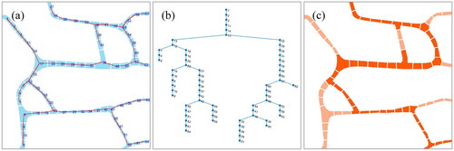
The weighting rules for the MSTP are as follows: An MST is defined as a subset of connected, edge-weighted, undirected graphs without cycles (Greenlaw and Hoover 1998) and with the smallest total edge weight. An MST can preserve the main structure of graph G. Using MSTP weights, the secondary branches of the river networks can be distinguished from the mainstream branches. The main steps in MST weighting are as follows: (1) Node classification: When a node is connected to only one other node, it is considered an end node. When a node is connected to two other nodes, it is considered an ordinary node. When a node is connected to three or more nodes, it is considered a hub node. A river segment can be formed by one hub node, one end node (or hub node), and several ordinary nodes. (2) Removal of short branches with a length less than l: Here, l is the length threshold of a path in an MST, which is equal to the number of edges on the path. In an MST, when an end node connects a hub node through s ($s\ge 0$) ordinary nodes, where s is the number of ordinary nodes, the edge set consisting of the end, ordinary, and hub nodes can be defined as a branch. For example, as shown in Figure 4(a), the red lines represent the MST generated from the constructed graph of the river network superpixels, and the blue numbers represent the number of nodes. In this MST, an end node N1 is connected to a hub node N17 by four ordinary nodes, namely N2, N3, N11, and N14, where the edge sets E(1, 2), E(2, 3), E(3, 11), E(11, 14), and E(14, 17) are branches that can be labeled as branch B(1, 17). A hub node typically connects several branches. For example, hub node N17 connects branches B(1, 17), B(12, 17), and B(57, 17). When a hub node is connected to t ($t\ge 2$) branches, p ($p=t-1$) branches exist and contain end nodes and q ($q=1$) branches exist and contain two hub nodes. The longest branches (length $L\le l$) that contain the end nodes should be preserved, and the remaining branches (length $L\le l$) that contain the end nodes must be eliminated (except for the hub nodes). For example, in Figure 4(b), the hub node N43 connects the following three branches: B(65, 43), B(64, 43), and B(23, 43). Branch B(23, 43) contains two hub nodes, N23 and N43. Branches B(65, 43) and B(64, 43) contain the end nodes, and the length of B(64, 43) is larger than that of B(65, 43). If $l=5,$ branches B(64, 43) and B(23, 43) should be preserved and branch B(65, 43) should be removed (except for hub node N43). When a hub node is connected with t ($t\ge 2$) branches, and among these branches, there exist p ($p\le t-2$) branches that contain end nodes and q ($q\ge 2$) branches with two hub nodes, all the branches (length $L\le l$) with end nodes should be removed (except for the hub nodes). (3) After removing the short branches, two types of superpixels pertain to superpixel sets X and Y, which are parts of the remaining branches and removed branches, respectively. The superpixels in sets X and Y have large and small weights, respectively. This is indicated by the weighting results colored in various shades of red in Figure 4(c), with darker colors representing larger weights. All weights are normalized based on the p-norm approach as follows: (1) $${\Vert w\Vert }_p={\left[\sum _{k=1}^N{\left|w_k\right|}^p\right]}^{1/p}$$(1) where p represents a positive real value, $\mathrm{\infty }$ or $\text{-}\mathrm{\infty }$ and N is the number of elements in the vector w. When $p=1,$ the 1-norm equals the sum of the absolute values of the vector; when $p=\mathrm{\infty },$ ${\Vert w\Vert }_{\infty }={\max }_i(|w(i)|).$ In this study, we set $p=\mathrm{\infty }$ to normalize the superpixel weights.

Figure 4. Weighting rules for minimum spanning tree pruning (MSTP) (a) Minimum spanning tree (MST) of the river network superpixels (b) Visualization of nodes and edges of the MST structure (c) Results of MSTP weighting for the river network.

3.2.2. Calculation of SP

The weighting rules for the SP are as follows: In a graph, the SP between two nodes is the path corresponding to the minimum sum of the weights of all edges that form the path. The number of times each node is traversed can be determined by calculating the SP between any two nodes. A large number indicates that the node is located at a centrally oriented position and is highly important. If the number of times node N is traversed is $S_n,$ we can set the corresponding SP weights of the river network superpixels as $SP=\{S_1,\mathrm{ }{S}_2,\mathrm{ }{S}_3,\mathrm{ }\dots ,\mathrm{ }{S}_n\}.$ To fuse different dimensions, all SP weights are normalized to [0, 1]. A high SP weight for a river network superpixel corresponds to a high pixel importance and centrality.

3.2.3. Calculation of ND

The ND weighting rules are as follows: The ND value of a node is equal to the number of adjacent edges that are connected to it. Assuming that the degree of node N is $D_n,$ we can set the corresponding ND weights of the river network superpixels as $ND=\{D_1,\mathrm{ }{D}_2,\mathrm{ }{D}_3,\mathrm{ }\dots ,\mathrm{ }{D}_n\}.$ To fuse the different dimensions, all the ND weights were normalized to [0, 1]. High ND weights for river network superpixels corresponded to important superpixels in terms of local connectivity.

3.2.4. Calculation of SA

The SA weighting rules are as follows: Assuming that the area of the superpixels at node N is $A_n,$ we can set the corresponding SA weights of the river network superpixels as $SA=\{A_1,\mathrm{ }{A}_2,\mathrm{ }{A}_3,\mathrm{ }\dots ,\mathrm{ }{A}_n\}.$ To fuse different dimensions, all SA weights are normalized to [0, 1]. High SA weights for river network superpixels corresponded to high river levels in these pixels.

The final weights of the river network superpixels were calculated using the following equation: (2) $$FW=k_1\times \mathit{MSTP}+k_2\times SP+k_3\times ND+k_4\times SA$$(2) where $k_1,$ $k_2,$ $k_3,$ and $k_4$ are the weight coefficients of the MSTP, SP, ND, and SA weights, respectively. The specific setting rules for these weight coefficients can be found in the discussion section of the experiments. According to the ranking of the FW values, superpixels at different levels of detail can be generated according to the ranking of FW values to obtain different sets of river network selection results. To avoid generating fractures, when the selected number of nodes in a river segment exceeds a fixed threshold, all nodes in this river segment are selected.

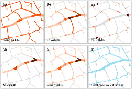
An example of river network superpixel weighting and selection is shown in Figure 5. Figures 5(a–d) show the MSTP, SP, ND, and SA weights of the river network superpixels, where a deeper color corresponds to a greater weight. Figure 5(e) shows the total weight results generated from the MSTP, SP, ND, and SA weights. Through weight ranking, we can apply superpixels with the highest weights for river selection. Figure 5(f) shows the final selection results for the river network. The blue and gray superpixels represent the selected and eliminated river network, respectively. The main and high-level rivers are well preserved, and the short and unimportant branches can be effectively removed.

Figure 5. Sample river network superpixel weighting and selection (a–e) The minimum spanning tree pruning (MSTP), shortest path (SP), node degree (ND), and superpixel area (SA), and total weight results, where the darker the color, the higher the weight (f) Results of river network selection based on weight ranking.

3.3. Elimination of redundant pixels at river network intersections

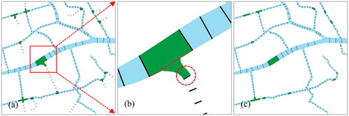
Because the unimportant branches were removed, the superpixels at the river network intersections became irregular and included redundant pixels. Consequently, the final elimination procedure was performed. As shown in Figure 6(a), the superpixels at river network intersections with redundant pixels are marked in green, and each superpixel has several intersecting segments such as black line segments. Based on the removed branches, redundant segments, such as the line segments marked with red circles in Figure 6(b), can be determined. By connecting the corresponding endpoints of the nonredundant line segments generated from the superpixels at the river network intersections, such as the red lines shown in Figure 6(b), the corresponding redundant pixels can be eliminated. Figure 6(c) shows the final selection results for this example, which were obtained using the proposed SRNS method after eliminating redundant pixels.

Figure 6. Elimination of redundant pixels at river network intersections.

4. Experiments and evaluation

4.1. Experiments involving rivers with mesh structures

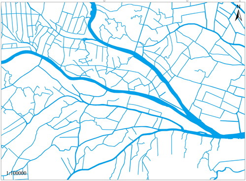
The original river networks considered in the selection experiments were located in Guangzhou Province, with data available in the 1:100000 basic geographic database of China. The latitude and longitude ranges of the experimental area were $22.540\le \mathit{Lat}\le 22.675$ and $113.307\le \mathit{Lon}\le 113.501,$ respectively. The original format of the polygonal river network was a vector format. The ArcGIS software (ESRI, USA) was used to convert the polygonal vector data into raster data with a resolution of 600 dpi. The size of the raster river network after format conversion was $7785\times 5662$ pixels (Figure 7). In this experimental area, the rivers exhibited typical grading phenomena, varying widths, and mesh structures.

Figure 7. The original raster river network in Guangzhou Province, China.

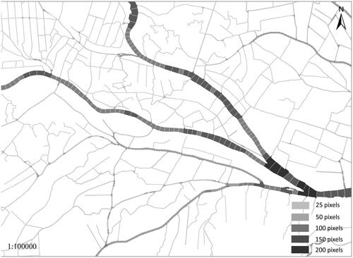
We divided the original raster river network into five levels by superpixel segmentation. Superpixel sizes used at the five levels were 25, 50, 100, 150, and 200 pixels according to the river width. The results of the multilevel superpixel segmentation of the raster river network used in this study are shown in Figure 8. After multilevel superpixel segmentation, the original raster river network was divided into 5345 superpixels of different sizes. A darker grey superpixel corresponds to a higher river level.

Figure 8. Results of multilevel superpixel segmentation for the raster river network.

According to the proposed SRNS method, the MSTP, SP, ND, and SA weights of the river network superpixels at two selection levels are shown in Figure 9, in which a darker color corresponds to a greater weight. At selection level 1 (a target scale of 1:150000), the original number of superpixels was 5345, and the corresponding weight coefficients were $k_1=5,k_2=2, k_3=2, \mathrm{and} k_4=100.$ The minimum length for short-branch removal was set to $sb=35,$ and the ratio of the selected superpixels was $r=0.75.$ At selection level 2 (a target scale of 1:250000), the original number of superpixels was 3950, and the corresponding weight coefficients were set to be the same as those set for level 1. The minimum length for short-branch removal was set to $sb=50,$ and the ratio of the selected superpixels was $r=0.75.$ In the actual experiment, the recommended settings for the weight coefficient were as follows: $k_4\ge k_1\ge k_2\ge k_3$ and $r=0.75.$ Notably, the different weights (MSTP, SP, ND, and SA) were associated with different functional characteristics. For example, the SA weight was used to distinguish the class of a river according to its width, thus requiring a relatively large weight coefficient $k_4.$ The MSTP and SP weights were used to maintain the global features of river networks in the same class, thus requiring the moderate weight coefficients $k_1$ and $k_2.$ The ND weight was used to determine the local features of river network intersections in the same class, and the corresponding weight coefficient $k_3$ 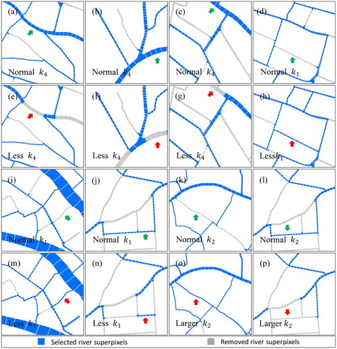was comparatively small. The weight coefficients used in these experiments were empirical values that were determined based on thousands of tests. If these weights are not arranged in the order given above, the corresponding features of the rivers will not be recognized and selection results will be affected. Figure 10 shows examples of selection results obtained using reasonable and inappropriate weight coefficients. When the weight coefficient $k_4$ is smaller than the other weight coefficients, the unreasonable removal of higher-level streams, such as the regions marked with arrows in Figures 10(a–c,e–g), can occur. When the weight coefficient $k_1$ is smaller than the weight coefficients $k_2$ and $k_3,$ many branches of the original river network are not removed as shown in the regions marked with arrows in Figures 10(d,h,i,m). This can also produce fractured branches, such as the regions marked with arrows in Figures 10(j,n). When the weight coefficient $k_2$ is large, the retention of redundant branches and the fracturing of the river network can occur, which is indicated by the regions marked with arrows in Figures 10(k–l,o–p).

Figure 9. MSTP, SP, ND, and SA weights for the river network superpixels at two different levels.

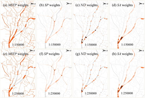
Figure 10. Examples of superpixel selection results using reasonable and inappropriate weight coefficients (a-d) Normal weight coefficients $k_4$ and $k_1$ (e-h) Small weight coefficients $k_4$ and $k_1$ (i-l) Normal weight coefficients $k_1$ and $k_2$ (m-n) Smaller weight coefficient $k_1$ and larger weight coefficient. $k_2$

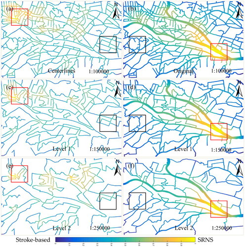
Using the proposed SRNS method, we generated selection results for the experimental river network at two target scales (1:150000 and 1:250000) (Figures 11(a–c)). The results showed that the proposed SRNS method could effectively maintain the main channels of the original rivers with large widths as illustrated for the studied river network at the two different levels of detail in region X. Additionally, short tributaries were removed during selection as shown in region Y. Specific examples are presented in Figure 12.

Figure 11. Results of river network selection with the proposed superpixel river network selection (SRNS) method and the stroke-based method. (a) The original raster river network (b-c) Selected results using the SRNS method at two different scales (d) The original vector river network (e-f) Selected results using the stroke-based method at two different scales.

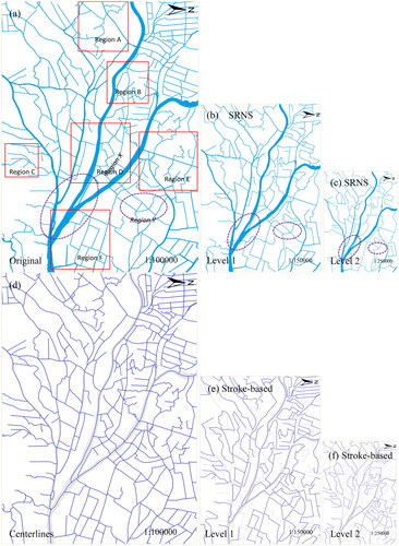
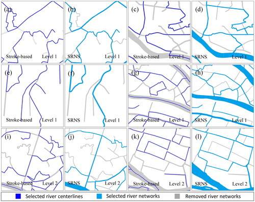
Figure 12. Detailed comparison of the selection results in regions a–f, as obtained using the stroke-based and proposed SRNS methods.

To quantitatively evaluate the proposed SRNS method, we used the stroke-based method (Yang et al. 2013, Zhao et al. 2020) to perform comparative experiments because it is a typical and widely used method designed for the selection of artificial linear features with mesh structures (Edwardes and Mackaness 2000, Heinzle et al. 2005, Yang et al. 2011, Li and Zhou 2012). Moreover, traditional river network selection methods have been designed only for natural rivers without mesh structures. Because the stroke-based method can only handle linear features without width information, we extracted the centerlines of the original river networks before implementing the stroke-based method. The centerline extraction method can be implemented using the ‘Collapse Dual Lines to Centerline’ tool in ArcGIS. Because this collapse tool was not sufficiently effective for managing complex river intersections, we performed a few manual editing procedures during the centerline extraction process. The results of the centerline extraction process are shown in Figure 11(d). It should be noted that the original river width information is lost. In many application scenarios, attribute information for areas of the river network that progressively vary in width does not exist, such as for river networks extracted from remote sensing images or scanned images. We compared the SRNS and stroke-based methods in this application scenario and set the corresponding weight threshold values at selection levels 1 and 2 to 0.25 and 0.5, respectively. In other words, the river ‘strokes’ with weights greater than these two values were selected. Figures 11(e,f) show the selection results at two target scales (1:150000 and 1:250000) as obtained using the stroke-based method. Compared with the proposed SRNS method, the stroke-based method exhibited several disadvantages when processing the river networks. We selected six typical regions (A–F) from the original experimental area to perform a detailed comparison of the selection results (Figure 11(a)). Figure 12 shows the detailed selection results in regions A–F obtained using the stroke-based and proposed SRNS methods. The removed and selected river portions are marked in gray and blue, respectively, and the following differences can be observed.

1. The connectivity of the original river networks obtained using the stroke-based method was disrupted and several isolated rings and river segments were generated as indicated in the selected river networks in Figures 12(e,g,i). The proposed SRNS method could effectively avoid this problem and ensure high connectivity as indicated by the selected river networks shown in Figures 12(f,h,j).

2. Because the stroke-based method ignored width information, it was difficult to maintain the original mainstream river network portions with large widths when using this method. The stroke-based method could occasionally maintain a wide mainstream area as shown in Figure 12(g). However, in several cases, only a part of the relatively wide mainstream river network, such as that shown in Figure 12(c), could be selected using the stroke-based method. In contrast, the proposed SRNS method could consistently preserve rivers with large widths at high levels by adjusting the SA weights as shown in Region B in Figures 12(d,h).

3. The original distribution uniformity of the stroke-based method could not be well preserved. For example, as shown in Figure 12(k), after the selection was performed using the stroke-based method, the river network portions located at the lower-left corner of the region were removed and those located at the upper-right corner were selected, which changed the distribution uniformity. In contrast, the proposed SRNS method could effectively achieve a uniform selection as indicated by the selection results shown in Figure 12(l).

4. The main structures of the original river networks could be effectively selected and redundant short branches could be removed using the proposed SRNS method as shown in Figures 12(b,f,j). The stroke-based method tended to destroy the original main structures of the river networks and often generated fractured river segments as shown in Figures 12(a,e,i).

Furthermore, because the quality of map generalization can be evaluated based on a similarity measure between the initial and generalized maps (Frank and Ester 2006, Filippovska et al. 2008, Podolskaya et al. 2009), three indicators were considered to evaluate the performance of and differences in the stroke-based and proposed SRNS methods: geometric similarity (GS), topological connectivity (TC), and distribution density (DD).

GS is widely used to examine consistencies in linear features before and after selection (Li and Zhou 2012) and can be defined as follows: (3) $${GS}_{\mathit{linear}}=\frac{M_l\cap N_l}{(M_l\cup N_l)-(M_l\cap N_l)}$$(3) where $M_l$ and $N_l$ indicate the lengths of the selected and original linear features, $\mathrm{respectively};$ $M_l\cup N_l$ indicates the total length of the selected and original linear features; and $M_l\cap N_l$ indicates the length of overlap between the selected and original linear features.

Similarly, the GS of areal features before and after selection can be defined as follows: (4) $${GS}_{\mathit{areal}}=\frac{M_a\cap N_a}{(M_a\cup N_a)-(M_a\cap N_a)}$$(4) where $M_a$ and $N_a$ indicate the areas of the selected and original areal features, $\mathrm{respectively};$ $M_a\cup N_a$ indicates the total area of the selected and original areal features; and $M_a\cap N_a$ indicates the area of overlap between the selected and original areal features.

When ${GS}_{\mathit{linear}}$ or ${GS}_{\mathit{areal}}$ is equal to 0 or 1, the similarity between the linear or areal features before and after selection is not consistent or completely consistent, respectively.

As shown in Table 1, we used ${GS}_{\mathit{linear}}$ to evaluate the selection results generated using the stroke-based method. The original length of the river network centerlines was 16,276 pixels, and the lengths of the selected river network centerlines at selection levels 1 and 2 were 12,104 and 9047 pixels, respectively. Similarly, ${GS}_{\mathit{areal}}$ was applied to the selection results generated using the proposed SRNS method. The original area of the river networks was 84,481 pixels, and the lengths of the selected river networks at selection levels 1 and 2 were 72,786 and 63,507 pixels, respectively. The GS values of the selection results obtained using the two methods were calculated according to the length and areal changes. According to Table 1, the GS values of the proposed SRNS method at selection levels 1 and 2 (0.862 and 0.752, respectively) were higher than those of the stroke-based method (0.743 and 0.556, respectively), which indicated that the proposed SRNS method could better maintain the GS than the traditional stroke-based method. This phenomenon occurred because the proposed SRNS method could consider the varying width information of the river network, and rivers at high levels were accurately selected, whereas the stroke-based method could only process the river network without width information.

Table 1. Quantitative evaluation of the selection results obtained using the stroke-based and proposed superpixel river network selection (SRNS) methods.

Method	Level	Original length/area	Selected length/area	Original segment /number of superpixels	Selected segment /number of superpixels	GS	TC
Stroke-based method	1 (1:150000)	16,276	12,104	1035	598 (57.8%)	0.743	0.145
	2 (1:250000)	16,276	9047	1035	391 (37.8%)	0.556	0.115
SRNS	1 (1:150000)	84,481	72,786	5345	3950 (73.9%)	0.862	1.000
	2 (1:250000)	84,481	63,507	5345	3018 (56.5%)	0.752	1.000

TC is applied to determine the degree of connection among the intersections of network structures and can be defined as follows: (5) $$TC=\frac{\sum _{a\in D}\sum _{b\in D;a\ne b}{R}_{ab}}{D(D-1)}$$(5) where $R_{ab}=1$ when nodes a and b are connected by a path, $R_{ab}=0$ when nodes a and b are not connected by a path, and D indicates the total number of pairs of nodes. When $TC$ is equal to 0 or 1, the TC of the network structure before and after selection is not reachable or completely reachable, respectively.

As shown in Table 1, the $TC$ indicator was calculated to measure the TC using the stroke-based and SRNS methods. The original number of river segments processed using the stroke-based method was 1035, and the selected numbers of river segments at selection levels 1 and 2 were 598 and 391, which accounted for 57.8% and 37.8% of all segments, respectively. The original number of river superpixels processed with the proposed SRNS method was 5345, and the selected numbers of river superpixels at selection levels 1 and 2 were 3950 and 3018, which accounted for 73.9% and 56.5% of all superpixels, respectively, which were higher than those for the stroke-based method. Notably, the river segments were divided into many superpixels in the proposed SRNS method, thus affecting the selection proportions. The TC values of the proposed SRNS method at the two selection levels (1.000 and 1.000, respectively) were higher than those of the stroke-based method (0.145 and 0.115, respectively), which suggested that the proposed SRNS method could better maintain TC than the traditional stroke-based method.

DD can be used to measure global distribution differences before and after selection, and it can be calculated according to the total number of overlaps with a fixed circular region centered at each pixel point. Figure 13 shows the density contrast in the river network selection results obtained using the proposed SRNS and stroke-based methods at the two selection levels. Both the stroke-based and SRNS methods could preserve the relative DD. For example, the original river network areas marked with red rectangles in Figures 12(a,b) were highly dense, and after selection using the two methods, the high-density portions of the river network located in the corresponding regions were preserved. Similarly, the low-density river network areas exhibited a low density after the selection as indicated by the regions marked with black rectangles in Figure 13.

Figure 13. Density contrast in the river network selection results obtained using the proposed superpixel river network selection and the stroke-based methods.

We also counted the percentage changes for rivers in different density ranges to measure differences between the stroke-based method and the proposed SRNS method in terms of density change (DC), and the results are shown in Table 2. Table 2 shows that (1) most rivers before and after selection using the two methods are in the density range of 0.2 –0.6. As the density level increased, the total density variation generated by the SRNS method increased from 8.2% to 16.2%, and the total density variation generated by the stroke-based method changed slightly (18.0% and 16.6%, respectively). (2) The average density change shown by the SRNS method (12.2%) at the two levels was lower than that shown by the stroke-based method (17.3%), which suggested that the proposed SRNS method had a better ability to preserve DD.

Table 2. Comparison of quantitative density changes based on the stroke-based and superpixel river network selection methods.

Density range		0–0.2	0.2–0.4	0.4–0.6	0.6–0.8	0.8–1.0	Sum
SRNS	Original	13.7%	29.9%	29.1%	15.8%	11.5%
	Level 1	16.6%	28.0%	29.4%	13.6%	12.4%
	DC	2.9%	1.9%	0.3%	2.2%	0.9%	8.2%
	Level 2	18.4%	27.3%	27.5%	11.9%	14.9%
	DC	4.7%	2.6%	1.6%	3.9%	3.4%	16.2%
Stroke-based	Original	9.9%	27.0%	36.6%	16.5%	10.0%
	Level 1	12.3%	33.6%	32.2%	12.9%	9.0%
	DC	2.4%	6.6%	4.4%	3.6%	1.0%	18.0%
	Level 2	12.4%	29.1%	28.3%	18.8%	11.4%
	DC	2.5%	2.1%	8.3%	2.3%	1.4%	16.6%

4.2. Experiments using rivers without mesh structures

The proposed SRNS method was tested using natural river networks without mesh structures. To evaluate the effectiveness of the SRNS method, the typical Delaunay-based method considering drainage areas proposed by Ai et al. (2006) and the top-down coding rule method considering connectivity proposed by Horton and Strahler (1952) for river network selection were applied to perform comparative experiments. Figure 14 shows the original natural river networks without a mesh structure and the selection results of the three methods.

Figure 14. Comparison between the proposed superpixel river network selection (SRNS) method and the typical Delaunay-based and coding-based methods. (a) The original natural river network (b-c) Selection results at two levels using the Delaunay-based method (d-e) Selection results at two levels using the coding-based method (f-g) Selection results at two levels using the proposed SRNS method.

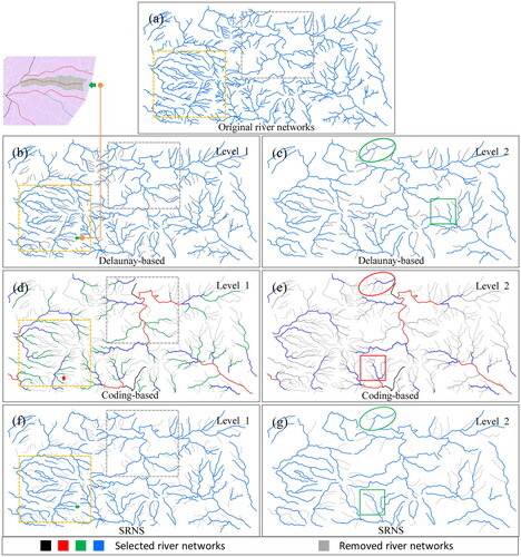
The proposed SRNS method maintained longer branches in distributary channels in the regions marked with green arrows and squares in Figures 14(f–g), whereas the Delaunay-based method could remove branches with small drainage areas, such as the regions marked with green arrows and squares in Figures 14(b–c). However, the coding-based method tended to remove all branches as shown in the regions marked with red arrows and squares in Figures 14(d–e). In terms of preserving the main channels, the coding-based method easily generated shorter channels when the original rivers had many branches as shown in the regions marked with red ellipses in Figure 14(e). In the same situation, the Delaunay-based and proposed SRNS methods could avoid this phenomenon as shown in the regions marked with green ellipses in Figures 14(c,g). In terms of preserving the density distribution, the Delaunay-based and proposed SRNS methods could maintain the original density differences among the different regions. The original high-density river networks still had a high density as shown in the areas marked with orange boxes in Figures 14(a,b,f), and low-density river networks still had a low density as shown by gray boxes in Figures 14(a,b,f). The coding-based method could not retain density differences after selection. For example, the original high-density area in Figure 14(d) became a low-density area.

In other words, the Delaunay-based and SRNS methods can appropriately retain branches and main channels, and both have advantages in maintaining the relative density of the network, whereas the coding-based method performs poorly in these three aspects. In addition, there is no evidence that the Delaunay- and coding-based methods can be applied to river networks with mesh structures; however, the proposed SRNS method can be used for river networks with or without mesh structures.

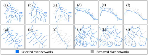
Because river networks have different patterns and structures (Kehew et al. 2013) under different geomorphological conditions, we tested the proposed SRNS method using dendritic, comb-like, skeleton-like, and radial river networks. Figure 15 shows the selection results for river networks with these patterns using the proposed SRNS method. For dendritic and comb-like river networks, the proposed SRNS method could progressively remove short branches at different levels of detail and preserve longer main channels as shown in Figures 15(a–f). For skeleton-like river networks, the longest skeleton structure was ultimately selected as shown in Figures 15(g–i). The main structural features of radial river networks could be well maintained by removing short branches at different levels of detail. In summary, the proposed SRNS method yielded a good selection effect for river networks with different patterns and structures.

Figure 15. Application of the proposed superpixel river network selection method to river networks with different patterns. (a-c) The original dendritic rivers and the selected results at two levels (d-f) The original comb-like rivers and the selected results at two levels (g-i) The original skeleton-like rivers and the selected results at two levels (j-l) The original radial rivers and the selected results at two levels.

5. Summary and future work

The varying widths of features in river networks can be used to distinguish the main channels and tributaries in these networks. The traditional vector-based selection method cannot be used for river networks with varying widths and thus may yield unreliable selection results. In this study, a raster-based selection method was proposed for river networks with varying widths based on superpixel segmentation. First, the multilevel division of the original raster river network was performed based on superpixel segmentation and corner detection. Subsequently, four types of weighting rules based on MSTP, SP, ND, and SA weights were designed for river superpixel selection. Finally, the redundant pixels at the river intersections were removed to generate hierarchical selection results. The following conclusions can be drawn by comparing the raster-based selection method with the traditional vector-based selection methods:

1. The proposed SRNS method can be used to effectively select river networks with varying widths and mesh structures that cannot be obtained using the traditional river selection methods.

2. The proposed SRNS method outperformed the traditional stroke-based selection method in preserving the main structure and connectivity of the river networks.

3. The relative distribution densities of the river networks were well maintained during selection when using the proposed SRNS method; thus, the proposed method could achieve uniform selection.

However, the proposed selection method for river networks has certain limitations. First, although the parameters used in the selection of river networks in different regions were different, all were set according to the rules recommended in this study. In the selection process, the weight coefficients needed to be adjusted several times to achieve optimal selection results. Techniques to automatically determine the optimal weight coefficients should be considered in future studies. Second, road elements are key linear features with mesh structures on a map, and related topics can be studied further based on the proposed superpixel-based selection method.

Disclosure statement

No potential conflict of interest was reported by the author(s).

Data and codes availability statement

The original river data and codes can be downloaded from https://github.com/Cartography0706/rivers

Additional information

Funding

This study was supported by the National Natural Science Foundation of China [Grant Number 42001402 and 42271454].

Notes on contributors

Yilang Shen

Yilang Shen received B.S. and Ph.D. degrees in geographical information systems from Wuhan University, in 2013 and 2019, respectively. His research interests include computer vision, map generalization and change detection of spatial data. He contributed to the concept, implementation and writing of this paper.

Rong Zhao

Rong Zhao received B.S., M.S. and Ph.D. degrees in geographic information systems from Wuhan University in 2014, 2016 and 2020, respectively. Her research interests include the deep learning and pattern recognition. She contributed to the concept, review and analysis of this paper.

Tinghua Ai

Tinghua Ai is a professor with the School of Resource and Environmental Sciences, Wuhan University. His research interests include multi-level representation of spatial data, map generalization, spatial cognition and spatial big data analysis. He contributed to the review and editing of this paper.

Fengfeng Han

Fengfeng Han received B.S. and M.S. degrees in geographic information systems from Shanxi Normal University and Wuhan University in 2013, and 2015, respectively. She is currently an engineer at the Shanghai WAYZ Technology Controls Ltd. She contributed to the discussion and analysis of this paper.

Su Ding

Su Ding received B.S. and Ph.D. degrees in geographic information systems from Wuhan University in 2015, and 2020, respectively. Her research interests include the geographic modeling and data mining. She contributed to the the discussion and analysis of this paper.

References

- Achanta, R., et al., 2012. SLIC superpixels compared to state-of-the-art superpixel methods. IEEE Transactions on Pattern Analysis and Machine Intelligence, 34 (11), 2274–2282.
- Ai, T., Ai, B., and Huang, Y., 2009. Multi-scale representation of hydrographic network data for progressive transmission over web. In: Proceedings of the 24th International Cartographic Conference. Santiago, Chile, 15–21 November.
- Ai, T., Liu, Y., and Chen, J., 2006. The hierarchical watershed partitioning and data simplification of river network. In: A. Riedl, W. Kainz, and G.A. Elmes, eds. Progress in spatial data handling. Berlin, Heidelberg: Springer, 617–632.
- Bergh, M., et al., 2012. “SEEDS: Superpixels Extracted via Energy-Driven Sampling.” In: A. Fitzgibbon et al. eds. European Conference on Computer Vision. Berlin: Springer, 13–26.
- Brewer, C.A., et al., 2013. Automated thinning of road networks and road labels for multiscale design of The National Map of the United States. Cartography and Geographic Information Science, 40 (4), 259–270.
- Buttenfield, B.P., Stanislawski, L.V., and Brewer, C.A., 2011. Adapting generalization tools to physiographic diversity for the united states national hydrography dataset. Cartography and Geographic Information Science, 38 (3), 289–301.
- Chen, J., et al., 2009. Selective Omission of Road Features Based on Mesh Density for Automatic Map Generalization. International Journal of Geographical Information Science, 23 (8), 1013–1032.
- Chabat, F., Yang, G.-Z., and Hansell, D.M., 1999. A Corner Orientation Detector. Image and Vision Computing, 17 (10), 761–769.
- Durighetto, N., et al., 2020. Intraseasonal drainage network dynamics in a headwater catchment of the Italian alps. Water Resources Research, 56 (4), e2019WR025563.
- Edwardes, A.J., and Mackaness, W.A., 2000. Intelligent Generalisation of Urban Road Networks. In: Proceedings, GIS Research UK 2000 Conference. York, April 5–7.
- Filippovska, Y., Walter, V., and Fritsch, D., 2008. Quality evaluation of generalization algorithms. ISPRS Commission II, WG II, 7.
- Frank, R., and Ester, M., 2006. A quantitative similarity measure for maps. In: Progress in spatial data handling. Berlin, Heidelberg: Springer, 435–450.
- Greenlaw, R., and Hoover, H.J., 1998. Fundamentals of the theory of computation: principles and practice. San Francisco, CA: Morgan Kaufmann.
- Han, Y., et al., 2020. Application of AHP to road selection. ISPRS International Journal of Geo-Information, 9 (2), 86.
- Harris, C.G., and Stephens, M., 1988. A combined corner and edge detector. In: 4th Alvey Vision Conference. Manchester, UK, 147–151.
- Guillon, H., et al., 2020. Machine learning predicts reach‐scale channel types from coarse‐scale geospatial data in a large river basin. Water Resources Research, 56 (3),
- Heinzle, F., Anders, K.H., and Sester, M., 2005. Graph based approaches for recognition of patterns and implicit information in road networks. In: Proceedings, 22th International Cartographic Conference. La Coruña, July 10–16.
- Herzog, S.P., Ward, A.S., and Wondzell, S.M., 2019. Multiscale feature‐feature interactions control patterns of hyporheic exchange in a simulated headwater mountain stream. Water Resources Research, 55 (12), 10976–10992.
- Horton, R.E., 1945. Erosional development of streams and their drainage basins; hydrophysical approach to quantitative morphology. Geological Society of America Bulletin, 56 (3), 275–370.2.0.CO;2]
- Huang, L., et al., 2017. A matrix-based structure for vario-scale vector representation over a wide range of map scales: the case of river network data. ISPRS International Journal of Geo-Information, 6 (7), 218.
- Jiang, B., and Claramunt, C., 2004. A structural approach to the model generalization of an urban street network. GeoInformatica, 8 (2), 157–171.
- Kehew, A.E., Lord, M.L., and Kozlowski, A.L., 2013. Glacial landforms | glaciofluvial landforms of erosion, In: S. A. Elias, C. J. Mock, eds. Encyclopedia of Quaternary Science. 2nd ed. Elsevier, 825–838.
- Kitchen, L., and Rosenfeld, A., 1982. Gray-level corner detection. Pattern Recognition Letters, 1 (2), 95–102.
- Levinshtein, A., et al., 2009. TurboPixels: Fast superpixels using geometric flows. IEEE Transactions on Pattern Analysis and Machine Intelligence, 31 (12), 2290–2297.
- Li, Z., and Chen, J., 2015. Superpixel segmentation using linear spectral clustering. In: Proceedings of the IEEE Conference on Computer Vision and Pattern Recognition. IEEE, 1356–1363.
- Li, C., et al., 2020. Selection method of dendritic river networks based on hybrid coding for topographic map generalization. ISPRS International Journal of Geo-Information, 9 (5), 316.
- Li, Z., 1994. Mathematical morphology in digital generalization of raster map data. Cartography, 23 (1), 1–10.
- Li, Z., and Zhou, Q., 2012. Integration of linear and areal hierarchies for continuous multi-scale representation of road networks. International Journal of Geographical Information Science, 26 (5), 855–880.
- Liu, H.-C., and Srinath, M.D., 1990. Corner detection from chain-code. Pattern Recognition, 23 (1-2), 51–68.
- Liu, M., et al., 2011. Entropy rate superpixel segmentation. In: 2011 IEEE Conference on Computer Vision and Pattern Recognition. IEEE, 2097–2104.
- Mackaness, W.A., and Beard, K.M., 1993. Use of graph theory to support map generalization. Cartography and Geographic Information Systems, 20 (4), 210–221.
- Mackaness, W.A., 1995. Analysis of urban road networks to support cartographic generalization. Cartography and Geographic Information Science, 22 (4), 306–316.
- McManamay, R.A., and DeRolph, C.R., 2019. A stream classification system for the conterminous United States. Scientific Data, 6 (1), 190017.
- Moore, A., et al., 2008. Superpixel lattices. In: 2008 IEEE Conference on Computer Vision and Pattern Recognition. IEEE, 1–8.
- Podolskaya, E.S., et al., 2009. Quality assessment for polygon generalization. In: A. Stein, W. Shi, and W. Bijke, eds. Quality Aspects in Spatial Data Mining, Chapter 16. Boca Raton, FL: CRC Press, 211–219.
- Schylberg, L., 1993. Computational methods for generalization of cartographic data in a raster environment. Doctoral thesis. Royal Institute of Technology, Department of Geodesy and Photogrammetry, Stockholm, Sweden.
- Shen, Y., et al., 2018. A new approach to simplifying polygonal and linear features using superpixel segmentation. International Journal of Geographical Information Science, 32 (10), 2023–2054.
- Shen, Y., et al., 2019. A polygon aggregation method with global feature preservation using superpixel segmentation. Computers, Environment and Urban Systems, 75, 117–131.
- Shen, Y., et al., 2022. Multilevel mapping from remote sensing images: a case study of urban buildings. IEEE Transactions on Geoscience and Remote Sensing, 60, 1–16.
- Shi, J., and Tomasi, C., 1994. Good features to track. In: Proceedings of the IEEE Conference on Computer Vision and Pattern Recognition, IEEE, 593–600.
- Shoman, W., and Gulgen, F., 2017. Centrality-based hierarchy for street network generalization in multi-resolution maps. Geocarto International, 32 (12), 1352–1366.
- Smith, S.M., and Brady, J.M., 1997. SUSAN-A new approach to low-level image processing. International Journal of Computer Vision, 23 (1), 45–78.
- Stanislawski, L.V., 2009. Feature pruning by upstream drainage area to support automated generalization of the United States National Hydrography Dataset. Computers, Environment and Urban Systems, 33 (5), 325–333.
- Strahler, A.N., 1952. Hypsometric (area-altitude) analysis of erosional topography. Geological Society of America Bulletin, 63 (11), 1117–1142.2.0.CO;2]
- Stum, A.K., Buttenfield, B.P., and Stanislawski, L.V., 2017. Partial polygon pruning of hydrographic features in automated generalization. Transactions in GIS, 21 (5), 1061–1078.
- Touya, G., 2007. River network selection based on structure and pattern recognition. In: 23rd International Cartographic Conference, Moscou, Russia.
- Touya, G., and Girres, J., 2013. Scalemaster 2.0: A scalemaster extension to monitor automatic multi-scales generalizations. Cartography and Geographic Information Science, 40 (3), 192–200.
- Veksler, O., Boykov, Y., and Mehrani, P., 2010. “Superpixels and Supervoxels in an Energy Optimization Framework.” In: K. Daniilidis, P. Maragos, and N. Paragios, eds. European Conference on Computer Vision. Berlin: Springer, 211–224.
- Yang, B., Luan, X., and Li, Q., 2011. Generating hierarchical strokes from urban street networks based on spatial pattern recognition. International Journal of Geographical Information Science, 25 (12), 2025–2050.
- Yang, M., Ai, T., and Zhou, Q., 2013. A method of road network generalization considering stroke properties of road object. Acta Geodaetica Et Cartographica Sinica, 2013 (04), 581–587.
- Yang, W., and Li, J., 2012. A method for rapid transmission of multi-scale vector river data via the internet. Geodesy and Geodynamics, 3 (2), 34–41.
- Yu, S., and Shi, J., 2003. Multiclass spectral clustering. In: International Conference on Computer Vision. IEEE, 313–319.
- Zhou, Q., and LI, Z., 2016. Empirical determination of geometric parameters for selective omission in a road network. International Journal of Geographical Information Science, 30 (2), 263–299.
- Zhao, R., Ai, T., and Wen, C., 2020. A method for generating variable-scale maps for small displays. ISPRS International Journal of Geo-Information, 9 (4), 250.