Understanding and extending the geographical detector model under a linear regression framework

Abstract

The Geographical Detector Model (GDM) is a popular statistical toolkit for geographical attribution analysis. Despite the striking resemblance of the q-statistic in GDM to the R-squared in linear regression models, their explicit connection has not yet been established. This study proves that the q-statistic reduces into the R-squared under a linear regression framework. Under linear regression and moderate-to-strong spatial autocorrelation, Monte Carlo simulation results show that the GDM tends to underestimate the importance of variables. In addition, an almost perfect power law relationship is present between the percentage bias and the degree of the spatial autocorrelations, indicating the presence of fast uplifting bias in response to increasing levels of spatial autocorrelations. We propose an integrated approach for variable importance quantification by bringing together the spatial econometrics model and the game theory based-Shapley value method. By applying our proposed methodology to a case study of land desertification in African, it is found human activity tends to affect land desertification both directly and indirectly. However, such effects appear to be underestimated or undistinguished in the classic GDM.

Keywords:

• Spatial autocorrelation
• geographical detector model
• variable importance decomposition

1. Introduction

The Geographical Detector Model (GDM), proposed by Wang et al. (2010), serves as a statistical toolkit for geographical attribution analysis by quantifying the extent to which the spatial variance of an outcome variable can be explained by a set of independent variables and their interactions (Wang et al. 2016). The distribution of most physical and human geographical variables often exhibits stark stratifications (Haining 2003, Banerjee et al. 2014, Dong et al. 2020), implying potential existence of distinct mechanisms operating across strata (Davies et al. 2005). The fundamental concept of GDM is spatially stratified heterogeneity that gauges the proportion of overall heterogeneity in an outcome variable attributed to between-strata heterogeneity, with strata delineated based on classifications of potential influencing factors (Wang et al. 2010, 2016). Should between-strata heterogeneity predominantly govern the total heterogeneity of an outcome variable, it is plausible to infer that the variable used to define strata is likely to be a driving factor of this outcome variable.

Mathematically, spatial stratified heterogeneity is quantified by the q-statistic, formulated as in Equation (1) $$q=1-\frac{\sum _{h=1}^L\sum _{i=1}^{N_h}{(y_{hi}-{\overline{y}}_h)}^2}{\sum _{i=1}^N{(y_i-\overline{y})}^2}=1-\frac{\sum _{h=1}^L{N}_h{\sigma }_h^2}{N{\sigma }^2};\mathrm{ }q\in [0,1],$$(1) (1)(1) $$q=1-\frac{\sum _{h=1}^L\sum _{i=1}^{N_h}{(y_{hi}-{\overline{y}}_h)}^2}{\sum _{i=1}^N{(y_i-\overline{y})}^2}=1-\frac{\sum _{h=1}^L{N}_h{\sigma }_h^2}{N{\sigma }^2};\mathrm{ }q\in [0,1],$$(1) (Wang et al. 2016), (1) $$q=1-\frac{\sum _{h=1}^L\sum _{i=1}^{N_h}{(y_{hi}-{\overline{y}}_h)}^2}{\sum _{i=1}^N{(y_i-\overline{y})}^2}=1-\frac{\sum _{h=1}^L{N}_h{\sigma }_h^2}{N{\sigma }^2};\mathrm{ }q\in [0,1],$$(1) where $h$ represents the $h$-th stratum predefined by the categories of one or more independent variables; $y_i$ is the outcome value of the $i$-th sample, and $\overline{y}$ is the overall mean; $y_{hi}$ is the outcome value of the $i$-th sample belonging to the $h$-th stratum and ${\overline{y}}_h$ is the sample mean of the $h$th stratum; $N_h$ and ${\sigma }_h^2$ are the sample sizes and variances of $y_{hi}$ for the $h$-th stratum, respectively; and parameters $N$ and ${\sigma }^2$ represent the size and variance of the full sample. The q-statistic lies within [0, 1], and its monotonic transformation, $\frac{N-L}{L-1}\frac{q}{1-q},$ is a classic F-statistic—the ratio of between-strata variance to within-strata variance of y, adjusted by corresponding degrees of freedom. This statistic conforms to a noncentral F-distribution, thereby enabling the undertaking of significance inference on the q-statistic. Detailed mathematical derivations on statistical significance test are given in referred to Wang et al. (2016). A q-statistic of substantial magnitude and statistical significance obtained for a given variable strongly suggests the potential role of that variable as a driving force behind the observed outcome variable.¹ Due to its intuitive constructionist logic and computational simplicity, GDM has been extensively applied to a wide range of social and environmental disciplines including, amongst others, urban studies (Feng et al. 2021, Sapena et al. 2021), ecology (e.g. Sannigrahi et al. 2020), environmental pollution (e.g. Ding et al. 2019, Zhang et al. 2019), and climate change studies (e.g. Yin et al. 2019, Fan et al. 2021). For instance, Zhang et al. (2019) categorized air pollution exposure time and intensity into a small number of bands, and investigated their main and interaction effects on peak bilirubin level of a newborn using GDM. Wang et al. (2023) employed the K-means clustering method to classify a set of factors into categories, and used GDM to quantify the impacts of those factors on vegetation optical depth.

Alongside the burgeoning applications of GDM, methodological advances have been proposed to address pragmatic issues when GDMs are applied to different types of spatial data. Cang and Luo (2018) used spatial variance to correct the bias of GDMs when spatially autocorrelated data are processed. They incorporate spatial weights into the GDM, that can cause the resulting values to exceed the range of [0, 1] and blur the physical interpretation of the value, while statistical significance can still be tested. To deal with the issue that users need to predefine (often arbitrarily) the discretization of a continuous variable (the number of categories as well as the cutting points), Meng et al. (2021) developed an optimal discretization scheme by an exhaustive search method. It has the advantage that it accounts for the characteristics of both independent and dependent variables, as opposed to focusing solely on independent variables.

Although the q-statistic bears a striking resemblance to the R-squared in linear regression, their explicit connection has not hitherto been established. This induces one of the key objectives and contributions of this study. Proving the equality that exists between the q-statistic and R-squared model fit statistic under a linear regression framework is crucial to understanding the mathematical nature of GDM and extending the methodology so that it can be applied to additional application contexts. To provide a proof of the concept, two types of extensions are discussed in this study. First, spatial autocorrelation affects the effective sample size, the information provided by independent or random geographic samples, and this in turn exerts influences on the calculations of both the overall and the stratum-wise variance parameters. It has been established that an effective sample size in the presence of spatial autocorrelation would be smaller than the actual geographic sample size (Griffith 2005, 2013). Using the equivalence between the q-statistic and R-squared, state-of-the-art spatial econometrics (or spatial statistics) models can be specified to deal with spatial autocorrelation, whilst retaining the logic instinct in their definition and measurement of variable contribution in GDM. In addition, many theoretically and mathematically sound variable importance decomposition methods, such as the game theory-based Shapley value method (Shapley 1953, Shorrocks 2013), could be naturally incorporated into spatial econometrics models. This would, in turn, offer informative interpretation of both the main and the interaction effects exerted from two or more independent variables on an outcome variable under investigation. It is important to note that establishing the equity which exists between the q-statistic and R-squared permits the extension advanced in this study to be readily applied to panel data models, leading to an important research avenue to be explored within future studies.

The equivalence between the q-statistic and R-squared can be first discerned through the genuine interpretation of these two statistics. At its heart, the q-statistic measures the extent to which independent variables explain the variability (or spatial pattern) of an outcome variable (Wang et al. 2010, 2016). Under the linear regression framework, the R-squared, also known as the coefficient of determination, measures the proportion of variability in a dependent variable that can be explained by independent variables included in a linear regression model (Kvalseth 1985, Freedman 2009).² Under conditions in which all independent variables were categorical in nature or had been categorized before entering a linear regression model, the R-squared measures exactly the same quantity as the q-statistic (mathematical details provided below). One key implication of this equality is that a more accurate q-statistic for spatial reasoning could be achieved in situations where data is not independent, as it would present spatial or group dependence. For instance, both classic and advanced spatial and multi-level extensions to the linear regression model have been well established and can be flexibly implemented with existing open-source software packages (e.g. Bates et al. 2015, Dong and Harris 2015, Dong et al. 2016, Bivand et al. 2021, Ma and Dong 2023). Such regression models combined with the game theory-based Shapley value method for variable importance decomposition can yield great benefits for spatial reasoning. To demonstrate the same, this study first derives the mathematical equivalence that exists between the q-statistic and the R-squared under a linear regression framework. Then, Monte Carlo simulation experiments are undertaken to assess the extent of the bias of the q-statistic in GDMs when processing data with varying degrees of spatial autocorrelation. One key result indicates that the q-statistic tended to underestimate the importance of factors; this downward bias elevates quickly in response to increasing levels of spatial autocorrelation. In addition, the empirical relationship that presents between the extent of bias and the strength of spatial autocorrelation exhibits a power law. Thereafter, the game theory-based Shapley value method, originally applied in non-spatial linear regression model is introduced to show how it could be adapted to spatial econometrics models. Finally, the developed methodology is applied to identify factor importance under the context of land desertification in Africa.

2. Proving the equivalence between the q-statistic and R-squared

The modelling starts with a classic linear regression model specified by Equation (2)(2) $$y_i=\alpha +\sum _{h=2}^L{\ddot{X}}_{h,i}{\gamma }_h+{\epsilon }_i {\epsilon }_i\sim N\left(0,\mathrm{ }{\sigma }_{{\epsilon }_i}^2\right),$$(2) as (2) $$y_i=\alpha +\sum _{h=2}^L{\ddot{X}}_{h,i}{\gamma }_h+{\epsilon }_i {\epsilon }_i\sim N\left(0,\mathrm{ }{\sigma }_{{\epsilon }_i}^2\right),$$(2) where $y_i$ is a dependent variable; $\alpha$ is the intercept term; ${\gamma }_h$ is the regression coefficient of covariates ${\ddot{X}}_{h,i};$ and ${\epsilon }_i$ is the residual term following a normal distribution with mean zero and variance ${\sigma }_{{\epsilon }_i}^2.$ It is useful to note that ${\ddot{X}}_{h,i}$ may be a set of dummy variables generated by encoding a categorical variable $X.$ Accordingly, if $X$ has or can be discretized into $L$ strata, then as many as $L-1$ dummy variables, ${\ddot{X}}_h,h\in 2, 3, \dots , L,$ need to be defined by (3) $${\ddot{X}}_h=\{\begin{array}{c}1\mathit{\text{ if }}{\ddot{X}}_{hi}\in \mathrm{hth} \mathrm{stratum}\\ 0 \mathrm{otherwise} \end{array}$$(3) The above assumes that any stratum of $X$ can be treated as the reference (i.e. baseline) group or category. Of course, any of the L strata can be selected as a reference group without affecting the estimates of the model. Among many of the assumptions imposed on the model residual term (an extensive list was referred to by Wooldridge (2010)), one of those is the independence of samples, or technically, the off-diagonal elements of the covariance matrix of ε must be equal to zero.

We turn our attention to the R-Squared statistic or the coefficient of determination formulated by Freedman (2009) as, (4) $$R^2=1-\frac{{\sum }_{i=1}^N{\left(y_i-{\widehat{y}}_i\right)}^2}{\sum _{i=1}^N{\left(y_i-\bar{y}\right)}^2},$$(4) where ${\widehat{y}}_i$ is the conditional expectation of $y_i$ given ${\ddot{X}}_i$ as in Equation (2)(2) $$y_i=\alpha +\sum _{h=2}^L{\ddot{X}}_{h,i}{\gamma }_h+{\epsilon }_i {\epsilon }_i\sim N\left(0,\mathrm{ }{\sigma }_{{\epsilon }_i}^2\right),$$(2) , and $\bar{y}$ is the overall mean of $y.$ This expression of R-Squared possesses most of the desirable properties that make a good statistic for model fit, and is easily extended to a model fit statistic that is resistant to extreme sample values (Kvalseth 1985). The numerator (the sum of residuals) stratum-wise can be further expressed as: (5) $$R^2=1-\frac{\sum _{h=1}^L\sum _{i=1}^{N_h}{(y_{hi}-{\widehat{y}}_{hi})}^2}{\sum _{i=1}^N{(y_i-\overline{y})}^2}$$(5) where N_h is the same as in Equation (1)(1) $$q=1-\frac{\sum _{h=1}^L\sum _{i=1}^{N_h}{(y_{hi}-{\overline{y}}_h)}^2}{\sum _{i=1}^N{(y_i-\overline{y})}^2}=1-\frac{\sum _{h=1}^L{N}_h{\sigma }_h^2}{N{\sigma }^2};\mathrm{ }q\in [0,1],$$(1) . Comparing Equation (5)(5) $$R^2=1-\frac{\sum _{h=1}^L\sum _{i=1}^{N_h}{(y_{hi}-{\widehat{y}}_{hi})}^2}{\sum _{i=1}^N{(y_i-\overline{y})}^2}$$(5) with the q-statistic expressed in Equation (1)(1) $$q=1-\frac{\sum _{h=1}^L\sum _{i=1}^{N_h}{(y_{hi}-{\overline{y}}_h)}^2}{\sum _{i=1}^N{(y_i-\overline{y})}^2}=1-\frac{\sum _{h=1}^L{N}_h{\sigma }_h^2}{N{\sigma }^2};\mathrm{ }q\in [0,1],$$(1) , there is only a need to prove the equality of ${\widehat{y}}_{hi}$ and ${\bar{y}}_h$ before establishing equality between the q-statistic and the R-squared. Recalling the coding rules for variable $X$ noted above, and with regard to the samples belonging to the $h$-th stratum, only ${\ddot{X}}_{hi}$ is equal to 1; the other dummy variables are equal to 0. Consequently, the predicted value, ${\widehat{y}}_{hi},$ is (6) $${\widehat{y}}_{hi}\left(X=h\right)={\widehat{y}}_{hi}\left({\ddot{X}}_{hi}=1,\mathrm{others}=0\right)=\mathrm{E}{y}_{hi}|\mathrm{ }{\ddot{X}}_{hi}=1,\mathrm{others}=0)=\widehat{\alpha }+{\widehat{\gamma }}_h$$(6) where $\widehat{\alpha }$ is the intercept and ${\widehat{\gamma }}_h$ is the estimated regression coefficient of ${\ddot{X}}_h.$ A well-known result is that the conditional expectation for samples to belong to the same group or stratum equals the group mean in dummy variable regression (e.g. Powers and Xie 2008, Freedman 2009), leading to (7) $${\widehat{y}}_{hi}=\mathrm{E}{y}_{hi}| {\ddot{X}}_{hi}=1,\mathrm{others}=0)={\bar{y}}_h.$$(7)

Derivations from this equity are provided in the Appendix. Finally, the equality between q-statistic and R-squared can be readily shown as (8) $$R^2=1-\frac{{\sum }_{i=1}^N{\left(y_i-{\widehat{y}}_i\right)}^2}{\sum _{i=1}^N{\left(y_i-\bar{y}\right)}^2}=1-\frac{\sum _{h=1}^L\sum _{i=1}^{N_h}{\left(y_{hi}-{\overline{y}}_h\right)}^2}{\sum _{i=1}^N{\left(y_i-\overline{y}\right)}^2}=1-\frac{\sum _{h=1}^L{N}_h{\sigma }_h^2}{N{\sigma }^2}=q.$$(8)

For multi-factor detection models, the above equivalence can be derived via a multivariate linear regression model. For example, two factors $X$ and $Z,$ each with three categories or strata are considered. In order to maintain the equality of R-squared and q-statistic, it is necessary to add interaction terms between the sets of dummy variables to the baseline regression model, leading to (9) $$\begin{array}{c}{y}_i=\alpha +{\gamma }_2{x}_{2i}+{\gamma }_3{x}_{3i}+{\beta }_2{z}_{2i}+{\beta }_3{z}_{3i}+ \mathit{Main} \mathit{effects}\\ {\delta }_{22}{\left(x_2{z}_2\right)}_i+{\delta }_{23}{\left(x_2{z}_3\right)}_i+{\delta }_{32}{\left(x_3{z}_2\right)}_i+{\delta }_{33}{\left(x_3{z}_3\right)}_i+{\epsilon }_i I\mathit{nteraction} \mathit{effects} \end{array}$$(9) where $\gamma$ and $\beta$ are regression coefficients for the two sets of dummy variables, x and z; $\delta$ is a vector of coefficients for the interactions between x and z. By Equation (7)(7) $${\widehat{y}}_{hi}=\mathrm{E}{y}_{hi}| {\ddot{X}}_{hi}=1,\mathrm{others}=0)={\bar{y}}_h.$$(7) again, the conditional expectation for samples to belong to the group j and k, ${\widehat{y}}_{jk},$ equals the group mean ${\overline{y}}_{jk}$ (Ab Abadie 2005, Athey and Imbens 2006), (10) $${\widehat{y}}_{jk}\left(X=j,Z=k\right)={\alpha +\widehat{\gamma }}_j+{\widehat{\beta }}_k+{\widehat{\delta }}_{jk}=\mathrm{E}\left(y_{i}X=j,Z=k\right)={\overline{y}}_h$$(10) where $j$ and $k$ are the factor levels of each variable. From this, it can be concluded that in a multi-factor interaction detection model, the equivalence between q-statistic and R-squared also holds.

After establishing the mathematical equivalence between the q-statistic and R-squared under a linear regression framework, simple verification with empirical data was then carried out using data in the R package of GDM (Wang et al. 2010). In a single factor detection model, with $\mathit{incidence}$ as the dependent variable and $\mathit{elevation}$ as the independent variable, the result of $q=R^2=0.6067$ was obtained. In a two-factor detection model with $\mathit{incidence}$ as the dependent variable, and $\mathit{soiltype} \text{and} \mathit{elevation}$ as the independent variable, the same equivalence of $q=R^2=0.6635$ was obtained. In addition, a series of Monte Carlo simulation experiments were carried out to verify the result. With correct linear regression model specifications, the R-squared obtained is equal to the q-statistic in GDM under all scenarios.

3. A Monte Carlo simulation experiment for data with spatial autocorrelation

After establishing the equivalence between the q-statistic and R-squared in the linear regression model, it was natural to study whether the q-statistic in GDM performs well in the presence of spatial autocorrelation. The rationale behind this was based on the established assumption that estimates of regression coefficients are biased in a linear regression model when applied to data with spatial autocorrelation (e.g. Anselin 1988, Banerjee et al. 2014). The biased estimates of regression coefficients for dummy variables discussed above could render Equation (7)(7) $${\widehat{y}}_{hi}=\mathrm{E}{y}_{hi}| {\ddot{X}}_{hi}=1,\mathrm{others}=0)={\bar{y}}_h.$$(7) invalid, thereby yielding bias in estimates of variable importance from the q-statistic because of the equivalence. To test this conjecture and assess the degree of bias of the q-statistic, a Monte Carlo simulation experiment was conducted. The specific steps of the experiment were as follows.

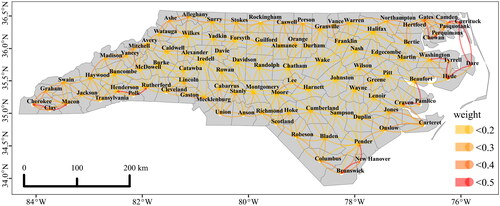
Step (1): Taking an open-source data, the North Carolina dataset associated with the spatialreg (Bivand et al. 2021) R package, as the experimental geography, the spatial adjacency based weights matrix $W$ was constructed, with elements ($w_{i,j}$) defined on the basis of geographical contiguity using Equation (11)(11) $$w_{i,j}=\{\begin{array}{c}1 \text{if areas }i\text{ and }j \text{share a border} \mathrm{and}\mathrm{ }i\ne j\\ 0 \mathrm{otherwise}\mathrm{ }\end{array}$$(11) . Afterwards, the weight matrix was row-normalized (Figure 1). (11) $$w_{i,j}=\{\begin{array}{c}1 \text{if areas }i\text{ and }j \text{share a border} \mathrm{and}\mathrm{ }i\ne j\\ 0 \mathrm{otherwise}\mathrm{ }\end{array}$$(11)

Figure 1. Topology of counties in North Carolina.

Step (2): An independent variable $X$ with three categories was generated, and the dependent variable y was then generated separately, by a spatial lag model (SLM), a spatial error model (SEM), and a spatial Durbin model (SDM): (12) $$\text{SLM}:y_i=\rho W\mathit{y}+\alpha +{\sum }_{h=2}^3{\ddot{X}}_{h,i}{\gamma }_h+{\epsilon }_i;{\epsilon }_i\sim N\left(0,{\sigma }_{\epsilon }^2\right)$$(12) (13) $$\text{SEM}:y_i=\alpha +{\sum }_{h=2}^3{\ddot{X}}_{h,i}{\gamma }_h+{\mu }_i;{\mu }_i=\rho W\mathit{\mu }+ {\epsilon }_i;{\epsilon }_i\sim N\left(0,{\sigma }_{\epsilon }^2\right)$$(13) (14) $$\text{SDM}:y_i=\rho W\mathit{y}+\alpha +{\sum }_{h=2}^3{\ddot{X}}_{h,i}{\gamma }_h+{\sum }_{h=2}^{3}W{\ddot{\mathit{X}}}_{\mathit{h}}{\phi }_h+{\epsilon }_i;{\epsilon }_i\sim N\left(0,{\sigma }_{\epsilon }^2\right)$$(14) where the strength of spatial autocorrelation increases with parameter $\rho ;$ ${\epsilon }_i$ is a normally distributed model residual term, with mean zero and variance ${\sigma }_{{\epsilon }_i}^2;$ $\alpha$ is the intercept term; and ${\ddot{X}}_h$ is the $h$-th dummy variable recoded from $X.$ In each simulation, the dependent variable, $\mathit{y},$ is generated based on different spatial autocorrelation mechanisms (SLM, SEM and SDM), randomly generated independent variables $X,$ randomly generated model residual term ${\epsilon }_i,$ and pre-set parameters. Without loss of generality, the simulation parameters were set as: (15) $$\begin{array}{c}\rho \in \mathrm{sequence}\left(\min =0.05,\max \hspace{0.17em}=0.95,\mathrm{interval}=0.05\right);{\epsilon }_i\sim N\left(0,\mathrm{ }0.1\right); X\sim U(1,3)\\ \alpha =1; \mathit{\gamma }=\left(1.5,\mathrm{ }1\right); \mathit{\phi }=(0.8, 0.5).\end{array}$$(15)

Step (3): The true variable importance quantities were calculated. With known values of the spatial autocorrelation parameter $\rho ,$ already set in Step (2), spatial econometrics models were degenerated to a linear regression model similar to Equation (2)(2) $$y_i=\alpha +\sum _{h=2}^L{\ddot{X}}_{h,i}{\gamma }_h+{\epsilon }_i {\epsilon }_i\sim N\left(0,\mathrm{ }{\sigma }_{{\epsilon }_i}^2\right),$$(2) with a new transformed dependent variable $\tilde{y}=y-\rho W\mathit{y}$ for SLM, $\tilde{y}=y-\rho W\mathit{y}+\rho W({\sum }_{h=2}^L{\ddot{X}}_{h,i}{\gamma }_h)$ for SEM, and $\tilde{y}=y-\rho W\mathit{y}$ for SDM. From this, the true variable importance quantity was calculated as, (16) $$R^2=1-\frac{\sum \left({\tilde{\mathrm{y}}}_i-{\widehat{\tilde{\mathrm{y}}}}_i\right)}{\sum \left({\tilde{\mathrm{y}}}_i-{\overline{\tilde{\mathrm{y}}}}_i\right)}=q\left(\tilde{y}\right|X)$$(16) where, ${\widehat{\tilde{\mathrm{y}}}}_i$ is the conditional expectation of ${\tilde{\mathrm{y}}}_i$ in a linear regression model.

Step (4): The percentage bias of the q-statistic in GDM was calculated as (17) $$\text{Percentage bias}= \frac{q-R^2}{R^2} .$$(17)

For each value of $\rho ,$ 1,000 samples were randomly generated and Steps (1) to (4) were implemented for each sample.

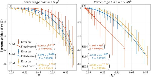
Monte Carlo simulation results are summarized in Figure 2(a and b). It is important to notice that the q-statistic in GDM tends to underestimate variable importance, and that the extent to which this downward bias is positively correlated with the strength of spatial autocorrelation. For instance, when $\rho$ equals 0.55 (a medium level of spatial autocorrelation), the q-statistic in GDM under-estimates variable importance by approximately 3% for SEM, 10% for SLM, and 20% for SDM. These biases quickly increase to 30% for SEM, 40% for SLM, and 50% for SDM in the presence of relatively strong spatial autocorrelation ($\rho$ equals 0.85). Another intriguing point is that an almost perfect power law relationship between the percentage bias and the degree of spatial autocorrelation tends to hold, with a Pearson correlation coefficient consistently exceeding 0.994. Turning the spatial autocorrelation parameter $\rho$ to the more commonly used Moran’s I statistic, the above findings still hold.

Figure 2. (a) The empirical relationship between strength of spatial auto-correlation ($\rho$) and percentage bias of q-statistic in GDM from three spatial econometrics models (true data generating processes). To avoid overlapping error bars, the curve of SEM is shifted 0.01 units to the left and the curve of SDM is shifted 0.01 units to the right; (b) The empirical relationship between Moran’s I and percentage bias of q-statistic in GDM under three spatial econometrics models. The same value of $\rho$ corresponds to different Moran’s I under three models. As a result, the starting and ending points of the three curves exhibit tiny differences.

This empirical power law functional form could be used to adjust the q-statistic if the GDM was chosen for identifying variable contributions. However, it is noted that this power law relationship is not expected to be over-interpreted as it might depend on geographic topology and mechanisms that generate spatial autocorrelation.³ On the other hand, the variable importance calculated from the SLM model estimates show positive bias and the percentage bias curve is almost indistinguishable from the zero line with a range of –0.5%, 0.2%. This was expected as the true data generating process followed an SLM model. However, the implication of this is that spatial econometrics models together with an adapted Shapley value method (discussed below) could serve as a useful alternative in spatial reasoning.

4. Adapting the game theory-based Shapley value method in spatial econometrics models

As demonstrated above, spatial econometrics models offer, compared to the GDM, greater accuracy for calculating variable importance with data that exhibits moderate to strong spatial dependency. In this section, a mathematically sound variable importance decomposition method, the game theory-based Shapley value method (Shapley 1953, Shorrocks 2013) is introduced into spatial econometrics models to offer flexible and intuitive interpretations of variable importance. In essence, the Shapley value method conceptualizes variables as ‘players’ in a collaborative game in which the optimal objective is to maximize ‘scores’ with respect to whether or not each player enters the game. Specifically, in a collaborative game with $N_p$ players, $p_i$ denotes i-th player (the i-th variable in a regression context). When $p_i$ participates in the game, the marginal contribution of $p_i$ is defined as following (Shorrocks 2013): (18) $$m\left({\mathit{P}}_{-i,j},p_i\right)=g\left({\mathit{P}}_{-i,j}+p_i\right)-g\left({\mathit{P}}_{-i,j}\right);i\in 1, 2,\dots ,N_v;j \in 1, 2,\dots ,2^{N_v}$$(18) where, $g()$ is a score function or gain function and ${\mathit{P}}_{-i,j}$ is j-th player-combination without $p_i.$ For example, in a game with 3 players, all player-combinations are: (19) $$\mathit{T} = \left\{\right(\varnothing ); (p_1); (p_2); (p_3); (p_1+p_2); (p_1+p_3);(p_2+p_3);(p_1+p_2+p_3\left)\right\}.$$(19)

It follows, that player-combinations without $p_3$ take the form: (20) $$\mathit{Q}\left(T,p_3\right)=\left\{\right(\varnothing ); (p_1); (p_2); (p_1+p_2\left)\right\}$$(20)

Naturally, when no players are involved in the game, the score $g\left(\varnothing \right)$ is equal to 0. Next, the Shapley value method calculates the ‘expected value’ of a player’s contribution to the game from the perspective of probabilities: (21) $$S\left(p_i\right)=\sum _{{\mathit{P}}_{-i,j}\in \mathit{Q}\left(\mathit{T},p_i\right)}\frac{\left(\left|{\mathit{P}}_{-i,j}\right|\right)!\left(N_v-\left|{\mathit{P}}_{-i,j}\right|-1\right)!}{N_v!}m\left({\mathit{P}}_{-i,j},p_i\right),$$(21) where, $\left|{\mathit{P}}_{-i,j}\right|$ denotes the number of players in $j$-th player-combination. For linear regression models, the R-squared value serves as the gain function, and as such, the marginal contribution of player $p_i$ in the SLM is expressed as follows: (22) $$m\left({\mathit{P}}_{-i,j},p_i\right)=R^2\left(y\sim \rho WY+{\mathit{P}}_{-i,j}+p_i\right)-R^2\left(y\sim \rho WY+{\mathit{P}}_{-i,j}\right),$$(22) where $R^2(·)$ indicates that R-squared values calculated based on parameter estimates from SLM.

We note that the Shapley value is an inherent method for the quantification of variable importance, and is independent of model estimation methods (Shorrocks 2013). All it requires is a proper model fit statistic that can measure scores or gains from combinations of independent variables after model estimation. The Shapley value method possesses several favorable attributes concerning the assessment of variable importance (Nandlall and Millard 2020). The first is non-discrimination; meaning that the variable’s importance remains unaffected by the order in which variables enter the model. Secondly, the Shapley value method measures the marginal contribution of each individual variable – variables and their interaction terms with more contributions assigned by higher Shapley values. Finally, the sum of the Shapley values of each variable is equal to the R-squared that occurs when all variables participate, ${\sum }_p^{N_v}S\left(p_i\right)=R^2({\mathit{P}}_{\mathit{all}}),$ and the contribution share of each variable can be derived as $S_{\%}\left(p_i\right)=\frac{S\left(p_i\right)}{R^2({\mathit{V}}_{\mathit{all}})}.$

5. A Case study of land desertification in Africa

Desertification is a process of land degradation which occurs under the combined actions of natural and human factors primarily in arid, semi-arid, and dry sub-humid areas. It significantly affects both the quality of local ecosystems and human life (Reynolds et al. 2007). The Sahel region represents a classic example of the same issue; the continuous deterioration of land desertification has been attributed to various climatic elements such as drought and strong winds, as well as to anthropogenic activities including deforestation and overgrazing. Despite the introduction of measures such as the Great Green Wall of Africa by Sahel nations to combat desertification and reverse its effects by 2030, progress is inadequate; largely due to the ongoing deforestation and unsustainable grazing practices being practiced by local residents (Zucca et al. 2022). Under the influence of global climate change, the Sahel region has experienced rising precipitation over the past 30 years; a crucial opportunity, all else being equal, for the region to regreen (Brandt et al. 2020). While consensus has been reached that desertification is affected by both climatic and human activity factors, the quantification of their relative contributions remains poorly understood. In this case study, we aim to narrow this gap by applying the developed method to assess the impacts of climatic factors, human activities, and their interplay on desertification in Great Green Wall of Africa.

Table 1 provides an overview of variables and data sources used in this investigation. Our outcome variable is a desertification index calculated for each grid (with a resolution of 0.5° × 0.5°) at year 2020 in the study area. The index is extracted by leveraging the albedo-Modified Soil-Adjusted Vegetation Index (MSAVI) feature space (Wu et al. 2019) through the Google Earth Engine. Population density and nighttime light intensity are included as proxy measures of human activities (Levin et al. 2020, Zucca et al. 2022). For climatic factors, we extract total precipitation and soil moisture variables from the European Centre for Medium-Range Weather Forecasts (ECMWF) Reanalysis V5 data (ERA5). All data has been resampled to a resolution of 0.5° × 0.5° under the WGS-84 coordinate system, and the independent variables are discretized into three categories using the natural breaks method. The final dataset is visualized in Figure 3.

Figure 3. Variables examined in the study: (a) Desertification index; (b) Nighttime lights intensity; (c) Population density; (d) Total precipitation; and (e) Soil moisture.

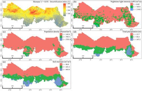
Table 1. Statistical summaries of variables used in this study’s models.

Factors	Unit	Mean	Variance	Data sources
Desertification index ($DI$)	1	171.507	7076.201	Google Earth Engine
Nighttime light intensity ($\mathit{ntl}$)	nW/cm^2/sr	4.971	182.744	NOAA-NGDC
Population density ($\mathit{pop}$)	Person/km^2	50.177	16495.87	ERA5
Total Precipitation ($\mathit{pre}$)	m	12.202	290.300	ERA5
Soil moisture ($sm$)	m^3/m^3	100.534	12136.690	ERA5

Note: The mean and variance of variables are calculated before the discretization procedure; NOAA-NGDC refers to National Oceanic and Atmospheric Administration’s National Geophysical Data Center.

The high value of Moran’s I (0.91 with a p-value $<$0.001) indicates the existence of strong spatial autocorrelation in the desertification index. This suggests that GDM might lead to biased estimates of variable importance. To ensure an appropriate form of spatial econometrics model, the commonly used Lagrange Multiplier Test (LM-test) was employed for model selection (Breusch and Pagan 1980). Significant LM-lag and LM-error values indicated that the spatial Durbin model (SDM) was a suitable choice (Table 2). To avoid the risk of model overfitting, the Akaike information criterion (AIC) is used to select a parsimonious model specification that yields good balance between model fit and model complexity (Akaike 1974). As shown in Table 3, Models 1 and 2 give similar AIC values that are significantly lower than those from other model specifications. As the R² value of Model 1 is higher than that of Model 2, we choose Model 1 as our preferred model for discussion.

Table 2. Estimation results on the LM-test.

Test	Value	p-value
LM-error	4478.1	0.000
LM-lag	4689.5	0.000
Robust LM-error	362.4	0.000
Robust LM-lag	573.7	0.000

Table 3. Estimation results on the Akaike information criterion and variable importance.

	Model specifications		AIC	R-squared values
Models	Main effects	Interaction effects	SDM	GDM	SDM
1	$\mathit{sm}+\mathit{ntl}$	$\stackrel{⃛}{\cap }(\mathit{sm},\mathit{ntl})$	29336.4	0.627	0.737
2	$pr+sm$	$\stackrel{⃛}{\cap }(pr,sm)$	29336.7	0.644	0.726
3	$pr+sm+\mathit{ntl}$	$\stackrel{⃛}{\cap }(pr,sm,\mathit{ntl})$	29346.6	0.661	0.747
4	$sm+\mathit{pop}$	$\stackrel{⃛}{\cap }(sm,\mathit{pop})$	29354.3	0.613	0.721
5	$sm+\mathit{pop}+\mathit{ntl}$	$\stackrel{⃛}{\cap }(sm,\mathit{pop},\mathit{ntl})$	29361.3	0.627	0.738
6	$pr+\mathit{ntl}$	$\stackrel{⃛}{\cap }(pr,\mathit{ntl})$	29361.8	0.554	0.686
7	$pr+sm+\mathit{pop}$	$\stackrel{⃛}{\cap }(pr,sm,\mathit{pop})$	29367.6	0.648	0.730
8	$pr+sm+\mathit{pop}+\mathit{ntl}$	$\stackrel{⃛}{\cap }(pr,sm,\mathit{pop},\mathit{ntl}$)	29387.6	0.663	0.748
9	$pr+\mathit{pop}$	$\stackrel{⃛}{\cap }(pr,\mathit{pop})$	29391.5	0.524	0.642
10	$pr+\mathit{pop}+\mathit{ntl}$	$\stackrel{⃛}{\cap }(pr,\mathit{pop},\mathit{ntl})$	29396.2	0.555	0.687
11	$\mathit{pop}+\mathit{ntl}$	$\stackrel{⃛}{\cap }(\mathit{pop},\mathit{ntl})$	29457.5	0.185	0.449

The symbol $\stackrel{⃛}{\cap }(·)$ denotes all possible interactions of variables, such as $\stackrel{⃛}{\cap }\left(a,b,c\right)=a\cap b+a\cap c+b\cap c+a\cap b\cap c.$

Table 4 presents estimation results on the relative importance and contribution share of variables from the preferred model—SDM with independent variables of soil moisture and nighttime light intensity. To facilitate comparison, estimation results from OLS and SLM models are also reported in Table 4. Overall, 73.7% of the variability in desertification is accounted for by the model, highlighting the substantial role of soil moisture and human activity in driving desertification in the study area. Turning to the contribution shares of each variable, it is not unanticipated to find that soil moisture alone contributes the most to desertification, accounting for over 50% of the model explanatory power. Human activity, measured by nighttime light intensity, also exhibits considerable influences on desertification, which is in accordance with the conclusions of previous studies on desertification (e.g. Wang et al. 2006, Jahelnabi et al. 2016).

Table 4. Decomposition results for variable importance.

Discretization	Variables	Shapley values			Contribution share (%)
		$S(\mathrm{OLS})$	$S(\mathrm{SLM})$	$S(\mathrm{SDM})$	$S_{\%}(\mathrm{OLS})$	$S_{\%}(\mathrm{SLM})$	$S_{\%}(\mathrm{SDM})$
Natural breaks	$\mathit{ntl}$	0.054	0.099	0.145	8.672	13.616	19.737
	$sm$	0.488	0.510	0.408	77.813	70.398	55.329
	$sm\cap \mathit{ntl}$	0.085	0.116	0.184	13.515	15.986	24.934
	total	0.627	0.725	0.737	100	100	100
Quantile	$\mathit{ntl}$	0.050	0.094	0.148	8.261	13.628	21.139
	$sm$	0.477	0.471	0.360	78.167	68.295	51.452
	$sm\cap \mathit{ntl}$	0.083	0.125	0.192	13.572	18.077	27.409
	total	0.611	0.690	0.700	100	100	100

OLS refers to ordinary least squares model and the R-squared (0.627) from the OLS model is equivalent to the q-statistic from the GDM.

As the Shapley value method treats each interaction term as a distinct variable that operates independently from the main effects, an interaction term possessing positive marginal contribution indicates an enhancement effect, whereas a negative marginal contribution suggests a trade-off effect. As shown in Table 4, the interaction effect between soil moisture and human activity accounts for approximately 25% of the model explanatory power, which is even slightly larger than the main effect of human activity on desertification. This suggests a significant anthropogenic enhancement effect on desertification, emphasizing the imperative to incorporate human activity intensity as an integral component when developing policies that aim to preserve land sustainability. To assess whether our empirical results are sensitive to different discretization methods, we once again cut independent variables into three groups using a quantile discretization method—representing the upper, middle, and lower thirds of their respective distributions. Encouragingly, the results exhibit a robust concordance between the two discretization methods (Table 4).

6. Conclusion

This study has established an explicit connection between the q-statistic in GDM and the R-squared in a linear regression model. By proving this equivalence, the state-of-the-art spatial econometrics models can be specified to deal with bias introduced by spatial autocorrelation in GDM, whilst retaining the logic inherent in the definition and measurement of variable contributions. The research combined the spatial econometrics models with a theoretically and mathematically sound variable importance decomposition method, the game theory-based Shapley value method, so that informative interpretations of the main and interaction effects exerted by two or more independent variables on an outcome variable could be ascertained. Through undertaking Monte Carlo simulation experiments the study demonstrated that GDM tended to underestimate variable importance, with the degree of downward bias being positively correlated with the strength of the spatial autocorrelation. In addition, an almost perfect power law relationship between the percentage bias and the degree of spatial autocorrelation tended to hold; indicating rapidly increasing bias in response to increasing levels of spatial autocorrelation. In contrast, variable importance calculated based on spatial econometrics model estimates presented minimal positive bias. This highlights the benefits of bringing together spatial econometrics models and the Shapley value method when it comes to spatial reasoning. By applying this study’s proposed methodology to a case study of land desertification in African, it was found that human activity tended to affect land desertification both directly (as indicated by a statistically significant main effect), and indirectly through enhancing the effects of climatic factors such as soil moisture. These effects appeared to be underestimated or indistinguishable in the classic GDM.

Despite this study’s advances, some limitations remain. First, the present study focuses on cross-sectional spatial econometrics models, thereby leaving more advanced spatio-temporal econometrics models untested. To address this in future, this study’s key findings should be interpreted in a cross-sectional setting. Secondly, the causal identification capabilities of GDM were not extended explicitly. This is primarily because causal identification relies more on research design than specific models.

Acknowledgment

The authors much appreciate the comments from the reviewers and editors, which improve the quality of the paper greatly.

Disclosure statement

No potential conflict of interest was reported by the author(s).

Data and codes availability statement

Data used in the empirical study and the R code for implementing the Monte Carlo simulation experiment are available for download at Figshare, https://doi.org/10.6084/m9.figshare.24196608.

Additional information

Funding

This study was supported by the National Natural Science Foundation of China [Grant Number 42001115 and 42101424].

Notes on contributors

Hang Zhang

Hang Zhang is a Ph.D. candidate at the Key Research Institute of Yellow River Civilization and Sustainable Development, Henan University, Kaifeng, China. His research interests include the development of spatial statistical models, urban remote sensing, and deep learning applications.

Guanpeng Dong

Guanpeng Dong is a Professor of Quantitative Human Geography at the Climate Change and Carbon Neutrality Lab and the Key Research Institute of Yellow River Civilization and Sustainable Development, Henan University, Kaifeng, China. His core research interests include the development of multi-level spatiotemporal statistical models and the application of these methods in global and local sustainable development analysis.

Jinfeng Wang

Jinfeng Wang is a Professor of spatial statistics at the State Key Laboratory of Resources and Environmental Information System, Institute of Geographic Sciences and Natural Resources Research, Chinese Academy of Sciences, Beijing, China. His research interests include methodological and theoretical development of spatial statistical models.

Tong-Lin Zhang

Tong-Lin Zhang is a Professor of Statistics at the Department of Statistics, Purdue University, USA. His research interests include asymptotics, Bayesian computation, physical science, and spatial analysis.

Xiaoyu Meng

Xiaoyu Meng received the Ph.D. degree in ecology from Chinese Academy of Sciences, Xinjiang, China. He is currently a Lecturer with the Key Research Institute of Yellow River Civilization and Sustainable Development, Henan University, Kaifeng, China. His research interests include spatial analysis, ecological remote sensing, machine learning, and geographic information science.

Dongyang Yang

Dongyang Yang received the Ph.D. degree in cartography and geographic information system from East China Normal University, Shanghai, China. He is currently an Associate Professor with the Key Research Institute of Yellow River Civilization and Sustainable Development, Henan University, Kaifeng, China. His research interests include spatiotemporal statistical modelling and aerosol remote sensing.

Yong Liu

Yong Liu received the Ph.D. degree in cartography and geographic information system from Sun Yat-sen University, Guangzhou, China. He is currently an Associate Professor with the Key Research Institute of Yellow River Civilization and Sustainable Development, Henan University, Kaifeng, China. His research interests include environmental economics and spatiotemporal statistical modelling.

Binbin Lu

Binbin Lu received the Ph.D. degree in cartography and geographic information system from National University of Ireland, Maynooth, Ireland. He is currently an Associate Professor at the School of Remote Sensing and Information Engineering, Wuhan University, Wuhan, China. His research interests include the development and application of geographically weighted modelling techniques.

Notes

1 We underscore that such associations are not supposed to be interpreted as causality without further examination. Establishing causality requires a robust research design, such as control laboratory experiments or quasi-natural experiments, which leverages strictly exogenous variations in an independent variable and links these variations to variability in an outcome variable under investigation (Angrist and Pischke 2010).

2 It is useful to note that the calculation of R-squared from a linear regression model can be varied, with different levels of desirable properties that make a good statistic for model fit (Kvalseth 1985, Freedman 2009). The interpretation of R-squared differs under a linear regression model and a generalized linear regression model; and so does its calculation. Detailed treatment of the R-squared is presented in McCullagh and Nelder (1989).

3 This study also carried out the simulation experiment on a regular grid topology with 50 by 50 cells. In addition, different forms of spatial weights matrix (adjacency- and distanced-based rules) were also tried Most of the results showed a power law relationship between the percentage bias from the q-statistic and the degree of spatial autocorrelation, but there were slightly different degrees of model fit; ranging from 0.91 to 0.998.

Appendix

This appendix provides the details of the derivations of the conclusion used in the main text, i.e. the conditional expectations that outcomes for samples belonging to the same group or stratum equal the group mean in a dummy variable OLS regression model. Without loss of generality, and assuming that the variable $X$ has or can be discretized into 4 categories, the corresponding dummy variables, $\ddot{\mathit{X}},$ are arranged in the order of categories: (1) $$\ddot{\mathit{X}}=\left[\begin{array}{cc}\left.\begin{array}{c}1,0,0,0\\ \cdots \end{array}\right\}& n_1\\ \left.\begin{array}{c}1,1,0,0\\ \cdots \end{array}\right\}& n_2\\ \left.\begin{array}{c}1,0,1,0\\ \cdots \end{array}\right\}& n_3\\ \left.\begin{array}{c}1,0,0,1\\ \cdots \end{array}\right\}& n_4\end{array}\right]=\left[\begin{array}{cccc}{1}_{n_1}& 0_{n_1}& 0_{n_1}& 0_{n_1}\\ 1_{n_2}& 1_{n_2}& 0_{n_2}& 0_{n_2}\\ 1_{n_3}& 0_{n_3}& 1_{n_3}& 0_{n_3}\\ 1_{n_4}& 0_{n_4}& 0_{n_4}& 1_{n_4}\end{array}\right]$$(1) where, $n_h$ is the number of samples in category-$h.$ The least squares estimation of $\mathit{\beta }$ is (2) $$\widehat{\mathit{\beta }}={\left({\mathit{X}}^{\mathbf{\text{'}}}\mathit{X}\right)}^{-1}{\mathit{X}}^{\mathbf{\text{'}}}\mathit{Y}=\left[\begin{array}{c}\frac{1}{n_1}\cdot \sum _i^{n_1}{y}_{n_{1}i}\\ -\frac{1}{n_1}\cdot \sum _i^{n_1}{y}_{n_{1}i}+\frac{1}{n_2}\cdot \sum _i^{n_2}{y}_{n_{2}i}\\ -\frac{1}{n_1}\cdot \sum _i^{n_1}{y}_{n_{1}i}+\frac{1}{n_3}\cdot \sum _i^{n_3}{y}_{n_{3}i}\\ -\frac{1}{n_1}\cdot \sum _i^{n_1}{y}_{n_{1}i}+\frac{1}{n_4}\cdot \sum _i^{n_4}{y}_{n_{4}i}\end{array}\right]$$(2) where, $n_{h}i$ is the i-th sample in category h. Then, the conditional expectation of $y_i$ is (3) $$\begin{array}{c}{\widehat{y}}_i=\left(1,x_{1i},x_{2i},x_{3i}\right)\cdot \widehat{\mathbf{\beta }}=\frac{1}{n_1}\cdot \sum _i^{n_1}{y}_{n_{1}i}+\left(-\frac{1}{n_1}\cdot \sum _i^{n_1}{y}_{n_{1}i}+\frac{1}{n_2}\cdot \sum _i^{n_2}{y}_{n_{2}i}\right)x_{2i}\\ +\left(-\frac{1}{n_1}\cdot \sum _i^{n_1}{y}_{n_{1}i}+\frac{1}{n_3}\cdot \sum _i^{n_3}{y}_{n_{3}i}\right)x_{3i}+\left(-\frac{1}{n_1}\cdot \sum _i^{n_1}{y}_{n_{1}i}+\frac{1}{n_4}\cdot \sum _i^{n_4}{y}_{n_{4}i}\right)x_{4i}\end{array}$$(3) which is the group mean. (4) $${\widehat{y}}_{hi}=\frac{1}{n_h}\cdot \sum _i^{n_h}{y}_{n_{h}i}={\overline{y}}_h$$(4)

References

- Ab Abadie, A., 2005. Semiparametric difference-in-differences estimators. The Review of Economic Studies, 72 (1), 1–19.
- Akaike, H., 1974. A new look at the statistical model identification. IEEE Transactions on Automatic Control, 19 (6), 716–723.
- Angrist, J.D., and Pischke, J.-S., 2010. The credibility revolution in empirical economics: How better research design is taking the con out of econometrics. Journal of Economic Perspectives, 24 (2), 3–30.
- Anselin, L., 1988. Spatial econometrics: Methods and models. Dorddrecht, The Netherlands: Kluwer Academic Publishers.
- Athey, S., and Imbens, G.W., 2006. Identification and inference in nonlinear difference-in-differences models. Econometrica, 74 (2), 431–497.
- Banerjee, S., et al., 2014. Hierarchical modeling and analysis for spatial data. Boca Raton, FL: Chapman and Hall/CRC.
- Bates, D., et al., 2015. Fitting linear mixed-effects models using lme4. Journal of Statistical Software, 67 (1), 1–48.
- Bivand, R., Millo, G., and Piras, G., 2021. A review of software for spatial econometrics in R. Mathematics, 9 (11), 1276. https://www.mdpi.com/2227-7390/9/11/1276
- Brandt, M., et al., 2020. An unexpectedly large count of trees in the West African Sahara and Sahel. Nature, 587 (7832), 78–82.
- Breusch, T.S., and Pagan, A.R., 1980. The lagrange multiplier test and its applications to model specification in econometrics. The Review of Economic Studies, 47 (1), 239–253.
- Cang, X., and Luo, W., 2018. Spatial association detector (SPADE). International Journal of Geographical Information Science, 32 (10), 2055–2075.
- Davies, K.F., et al., 2005. Spatial heterogeneity explains the scale dependence of the native–exotic diversity relationship. Ecology, 86 (6), 1602–1610.
- Ding, Y., et al., 2019. Using the geographical detector technique to explore the impact of socioeconomic factors on PM2.5 concentrations in China. Journal of Cleaner Production, 211, 1480–1490.
- Dong, G., and Harris, R., 2015. Spatial autoregressive models for geographically hierarchical data structures. Geographical Analysis, 47 (2), 173–191.
- Dong, G., et al., 2016. Spatial random slope multilevel modeling using multivariate conditional autoregressive models: a case study of subjective travel satisfaction in Beijing. Annals of the American Association of Geographers, 106 (1), 19–35.
- Dong, G., et al., 2020. Developing a locally adaptive spatial multilevel logistic model to analyze ecological effects on health using individual census records. Annals of the American Association of Geographers, 110 (3), 739–757.
- Fan, X., et al., 2021. Future climate change hotspots under different 21st century warming scenarios. Earth’s Future., 9 (6), e2021EF002027.
- Feng, R., et al., 2021. Urban ecological land and natural-anthropogenic environment interactively drive surface urban heat island: an urban agglomeration-level study in China. Environment International, 157, 106857.
- Freedman, D.A., 2009. Statistical models: theory and practice. Cambridge, UK: Cambridge University Press.
- Griffith, D.A., 2005. Effective geographic sample size in the presence of spatial autocorrelation. Annals of the Association of American Geographers, 95 (4), 740–760.
- Griffith, D.A., 2013. Establishing qualitative geographic sample size in the presence of spatial autocorrelation. Annals of the Association of American Geographers, 103 (5), 1107–1122.
- Haining, R., 2003. Spatial data analysis: theory and practice. Cambridge, UK: Cambridge University Press.
- Jahelnabi, A.E., et al., 2016. Assessment of the contribution of climate change and human activities to desertification in Northern Kordofan-Province, Sudan using net primary productivity as an indicator. Contemporary Problems of Ecology, 9 (6), 674–683.
- Kvalseth, T.O., 1985. Cautionary Note about R2. The American Statistician, 39 (4), 279–285.
- Levin, N., et al., 2020. Remote sensing of night lights: a review and an outlook for the future. Remote Sensing of Environment, 237, 111443.
- Ma, J., and Dong, G., 2023. Periodicity and variability in daily activity satisfaction: toward aa space-time modeling of subjective well-being. Annals of the American Association of Geographers, 113 (8), 1918–1938.
- McCullagh, P., and Nelder, J.A., 1989. Generalized linear models (second edition). Boca Raton, FL: Chapman & Hall/CRC.
- Meng, X., et al., 2021. Development of a multiscale discretization method for the geographical detector model. International Journal of Geographical Information Science, 35 (8), 1650–1675.
- Nandlall, S.D., and Millard, K., 2020. Quantifying the relative importance of variables and groups of variables in remote sensing classifiers using Shapley values and game theory. IEEE Geoscience and Remote Sensing Letters, 17 (1), 42–46.
- Powers, D., and Xie, Y., 2008. Statistical methods for categorical data analysis. Bingley, UK: Emerald Group Publishing.
- Reynolds, J.F., et al., 2007. Global desertification: building a science for Dryland development. Science, 316 (5826), 847–851.
- Sannigrahi, S., et al., 2020. Responses of ecosystem services to natural and anthropogenic forcings: a spatial regression based assessment in the world’s largest mangrove ecosystem. The Science of the Total Environment, 715, 137004.
- Sapena, M., et al., 2021. Estimating quality of life dimensions from urban spatial pattern metrics. Computers, Environment and Urban Systems, 85, 101549.
- Shapley, L.S., 1953. A value for n-person games. In: H. Kuhn, and A. Tucker, eds., Contributions to the theory of Games II. Princeton, NJ: Princeton University Press.
- Shorrocks, A.F., 2013. Decomposition procedures for distributional analysis: a unified framework based on the Shapley value. The Journal of Economic Inequality, 11 (1), 99–126.
- Wang, H., et al., 2023. Seasonal variations in vegetation water content retrieved from microwave remote sensing over Amazon intact forests. Remote Sensing of Environment, 285, 113409.
- Wang, J., et al., 2010. Geographical detectors‐based health risk assessment and its application in the neural tube defects study of the Heshun Region, China. International Journal of Geographical Information Science, 24 (1), 107–127.
- Wang, J., Zhang, T., and Fu, B., 2016. A measure of spatial stratified heterogeneity. Ecological Indicators, 67, 250–256.
- Wang, X., Chen, F., and Dong, Z., 2006. The relative role of climatic and human factors in desertification in semiarid China. Global Environmental Change, 16 (1), 48–57.
- Wooldridge, J.M., 2010. Econometric analysis of cross section and panel data (second edition). Cambridge, MA: MIT press.
- Wu, Z., et al., 2019. Study of the desertification index based on the albedo-MSAVI feature space for semi-arid steppe region. Environmental Earth Sciences, 78 (6), 232.
- Yin, Q., et al., 2019. Mapping the increased minimum mortality temperatures in the context of global climate change. Nature Communications, 10 (1), 4640.
- Zhang, L., et al., 2019. Air pollution exposure associates with increased risk of neonatal jaundice. Nature Communications, 10 (1), 3741.
- Zucca, C., et al., 2022. Land degradation drivers of anthropogenic sand and dust storms. CATENA, 219, 106575.