Importance of factors driving firms’ decisions on spatial distribution structures

ABSTRACT

The design of a spatial distribution structure is of strategic importance for companies, to meet required customer service levels and to keep logistics costs as low as possible. Spatial distribution structure decisions concern distribution channel layout – i.e. the spatial layout of the transport and storage system – as well as distribution centre location(s). This paper examines the importance of seven main factors and 33 sub-factors that determine these decisions. The Best-Worst Method (BWM) was used to identify the factor weights, with pairwise comparison data being collected through a survey. The results indicate that the main factor is logistics costs. Logistics experts and decision makers respectively identify customer demand and service level as second most important factor. Important sub-factors are demand volatility, delivery time and perishability. This is the first study that quantifies the weights of the factors behind spatial distribution structure decisions. The factors and weights facilitate managerial decision-making with regard to spatial distribution structures for companies that ship a broad range of products with different characteristics. Public policy-makers can use the results to support the development of land use plans that provide facilities and services for a mix of industries.

KEYWORDS:

• Spatial distribution structure
• distribution channel layout
• distribution centre location
• warehouse location
• Best-Worst Method (BWM)

1. Introduction

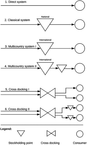
Distribution refers to the steps involved in the transportation and storage of goods, from supplier to customer in a supply chain (Chopra 2003). To meet the required service levels, it is of strategic importance for companies (e.g. shippers and logistics service providers – LSPs) to select the optimal distribution channel layout – i.e. the spatial layout of the transport and storage system – to serve customer needs and keep logistics costs low (Ashayeri and Rongen 1997; Baker 2006; Verhetsel et al. 2015). Together, the distribution channel layout and choice of distribution centre (DC) location(s) are known as the decision on spatial distribution structures. Figure 1 shows typical layouts. Products can be transported directly from the manufacturer (layout 1 in Figure 1), from central DC locations (layouts 2 and 3 in Figure 1), from cross-dock DCs (layout 5), or from multiple (regional or local) DC locations to the customer (layout 4 and 6). These configurations and DC locations will produce very different results in terms of customer order lead-time and various logistics cost components, including inventory costs and transport costs.

Figure 1. Distribution channel layouts (based on Kuipers and Eenhuizen 2004).

Spatial distribution structures are affected by a wide array of factors, ranging from customer requirements concerning service levels and delivery costs, to specific location attributes and the broader institutional environment in which the company has to operate (Chopra 2003; Cooper 1984; Korpela et al. 2001; McKinnon 1984; Picard 1982; Wanke and Zinn 2004). These factors affect decisions in a variety of ways. Volatile demand, for example, drives companies towards a central DC layout, allowing them to pool inventory risks, while high service level requirements, for example including same-day deliveries, drive companies towards a decentralised layout that allows them to cut delivery times. The aim of this paper is to provide insight into the importance of the various factors involved in choosing the optimal spatial distribution structure. We examine whether there are factors of general importance to decision-makers – i.e. decision-makers affiliated to companies in diverse industries – and experts. Knowing these factors is particularly relevant when it comes to designing spatial distribution structures for companies shipping multiple products with diverse characteristics, for example low value and high value products. Our research can also help policy-makers develop land use plans designed to attract companies from diverse industries. Furthermore, our research should help scientists and consultants to improve DC location models, which often use incomplete factor sets or incorrect factor weights (Mangiaracina, Song, and Perego 2015). Despite a clear need for this type of knowledge, there is a lack of empirical research into the factors that drive companies’ spatial distribution structure decision (Onstein et al., 2019). Traditional distribution network design models are prescriptive, often using optimisation methods to calculate the optimal distribution layout (Meixell and Gargeya 2005; Olhager, Pashaei, and Sternberg 2015). Mangiaracina, Song, and Perego (2015), for example, found that only five out of 126 reviewed studies include empirical research. To the best of our knowledge, Song and Sun (2017) are the only authors to have developed and tested a descriptive framework (including 15 factors) on supply chain network design, looking at the factors behind combined supply chain functions, including sourcing, production and distribution locations, although not identifying the unique contribution these factors have on the distribution-related decisions. As such, our study is the first to address the importance of factors that exclusively determine the selection of a spatial distribution structure. Although the location choice for DCs has attracted more empirical research (e.g. Dablanc 2013; Hesse 2004; McKinnon 2009; van den Heuvel et al. 2013; Verhetsel et al. 2015), none of the studies involved includes all the relevant factors. Our study contributes to existing literature by identifying a holistic set of factors and by empirically testing their importance.

Our main research questions are: (1) what are the main factors that determine companies’ spatial distribution structure decision? and (2) how important are these factors, relative to each other? To answer these questions, first, a descriptive framework was developed based on existing literature, after which the relative importance of the factors involved was measured, using the Best-Worst Method (BWM) to determine the factor weights. BWM is a suitable method to quantify factor weights, because it requires fewer pairwise comparison data than matrix-based multi-criteria decision-making methods (Rezaei 2015). An online survey was used to collect the data from two populations: (1) Decision-makers on spatial distribution structures and (2) Experts.

The remainder of the paper is organised as follows. Section 2 reviews relevant literature and presents a set of factors that drive the selection of spatial distribution structures. In Section 3, the Best-Worst Method and the survey data collection procedure are addressed, while the results are discussed in Section 4, and the conclusions, practical implications, research limitations and suggestions for future research are presented in Section 5.

2. Decision factors

This section discusses the main factors and the underlying factors (sub-factors) on the basis of a systematic literature review. A summary of all the factors is presented in Table 2 at the end of this section.

We set up a systematic literature review panel (Tranfield, Denyer, and Smart 2003), including a PhD student and two Logistics professors. The context of the literature review was spatial distribution structure selection. The selection criteria focus on spatial distribution structures, i.e. factors that drive distribution channel layout and distribution centre location selection. Studies that do not deal with factors driving the spatial distribution structure decision were excluded. Furthermore, only studies are included that aim to identify the factors or explain their influence. Studies that only list factors, for example, as a preparation for quantitative modelling, were not included. Several databases (i.e. ScienceDirect, Google Scholar, Emerald and Scopus) were used to search for specific keywords (i.e. spatial distribution structure, distribution channel layout, distribution network design, DC location, warehouse location, etc.) and strings – for example, ‘factors distribution channel layout’. Backward snowballing and forward snowballing resulted in more relevant publications. 52 academic publications were selected for in-depth examination (40 papers, three PhD theses, three conference proceedings, four academic book chapters, one working paper and one Master thesis). The studies in question involve supply chain management, (economic) geography and transportation disciplines. The use of academic literature increases the validity of the factor selection, i.e. indicating that the factors being included are indeed important factors. The factors were selected from the publications either because they were listed in a table containing the influencing factors, or because they were mentioned in the text of the publication. Selecting factors from 52 studies can be problematic when there are differences in population or study context. However, when the importance of a factor is confirmed by multiple studies with different contexts and research methods (e.g. quantitative models, surveys, interview-based), it may be assumed that it is indeed an important factor (Rousseau, Manning, and Denyer 2008).

We reduced the original literature-based list of 48 factors to a smaller set of 33 factors (Table 2), taking into account the time constraints related to filling out a survey. We selected 32 factors based on the number of literature references, i.e. factors with only one or two references (for example cost of living) were excluded. To validate the importance of the factors that were identified, nine experts were asked for their opinion on the 20 most important factors, 19 of which were already included in the set of 32 factors. Although the factor ‘perishability’ receives relatively little attention in relevant literature, it is added because six (of nine) experts argue that it is an important factor. All nine experts are decision-makers on spatial distribution structures or researchers with over five years of experience on spatial distribution structure selection in diverse industry sectors. The experts were selected from our own network and approached by email. Twenty experts were approached. Nine experts agreed to give their opinion. Seven out of nine experts are from academia and two out of nine experts from industry. Table 1 presents an overview of the experts’ expertise.

Table 1. Expertise of logistics experts for factor validation.

Expert	Expertise
1	Full professor Freight and Logistics and principal scientist with over 20 years of experience on research projects within diverse industries, e.g. automotive, fashion, food and aviation
2	Assistant professor Transport and Logistics, applied researcher and consultant with 18 years of experience in diverse industries, e.g. office retail sector, humanitarian supply chains and oil&gas
3	Assistant professor Transport and Logistics, experience with supervising MSc thesis in several industry sectors
4	Assistant professor Transport and Logistics, experience with research on location selection for city distribution centres
5	Assistant professor Operations and Supply Chain Management with over 10 years of experience on research projects in several industries, e.g. aviation, high-tech, tourism, oil&gas as well as research on facility location selection
6	Professor of Logistics and Operations Management with over 20 years of research on warehousing as well as consultancy on DC location selection
7	Senior researcher on (sea)freight transport and spatial logistics processes. Research project (2014) that analyses spatial logistics and economic development in two European regions
8	Logistics director of supermarket chain – decision-maker with 25 years of experience in the food sector
9	Director of Port Innovation – decision-maker with experience in development of industrial clusters

2.1. Demand factors

Three demand-related factors are distinguished from literature: (1) demand level, (2) demand dispersion – geographical dispersion of customers over the company’s target market – and (3) demand volatility (Christopher 2011; Vos 1993). Customer demand level influences the number of DCs needed to deliver customer orders in time. A high demand level involves daily customer orders, while a low demand level involves customer orders less than once a month. High demand volatility implies that customer demand levels fluctuate on a monthly basis. Low demand volatility implies that demand levels are stable over a period of at least six months. In the case of geographically dispersed customer demand, mixed layouts have two advantages: (1) reduced inventory risks and (2) the possibility of quick deliveries using regional DCs. In the case of high demand volatility, it is better to use a layout with few DC locations, to reduce inventory costs (Chopra 2003; Mangiaracina, Song, and Perego 2015).

2.2. Service level factors

Five important service level factors are: (1) supplier lead-time, (2) delivery time, (3) delivery reliability, (4) responsiveness and (5) returnability. Delivery time is defined as ‘time from [customer] order placement to customer delivery – in days’ (Wanke and Zinn 2004, 470). Delivery times are influenced by transport mode and delivery frequency (Mangiaracina, Song, and Perego 2015). The type of product determines the delivery times customers are willing to accept. They do not accept long delivery times for substitutable products, which motivates companies to choose decentralised layouts. Delivery reliability is imperative for companies distributing high-value goods. Responsiveness is the reaction speed and flexibility in meeting customer demand (Christopher 2011). A decentralised layout and fast transport modes increase a company’s responsiveness (Chopra 2003). Returnability refers to ‘the ease with which a customer can return unsatisfactory merchandise and the ability of the network to handle such returns’ (Chopra 2003, 124). Decentralised layouts (for example Layout 4, Figure 1) offer customers flexible return options. In the e-commerce era, returnability has become an important service element (Hjort and Lantz 2016).

2.3. Product characteristics factors

There are three product factors that influence the spatial distribution structure decision: (1) Product value density, (2) Package density and (3) Perishability. High value products are associated with high inventory costs, motivating companies to choose a centralised layout (Christopher 2011; Wanke and Zinn 2004). Products with a low value density are often easily substituted, which means they have to be available locally and motivates companies to choose a layout with local DCs (Ashayeri and Rongen 1997). Packaging density (number of products per m³) influences handling and inventory costs. High perishability – i.e. shelf life length in months (Wanke and Zinn 2004, 470) – may motivate companies to choose a distribution channel layout without storage or with cross docking – for example layout 5 or 6 (Figure 1).

2.4. Logistics costs factors

Based on existing literature, four leading logistics costs factors can be identified: (1) inbound transport costs, (2) outbound transport costs, (3) inventory costs and (4) warehousing costs. Many authors emphasise the importance of logistics costs factors (see e.g. Ashayeri and Rongen 1997; Chopra 2003; Christopher 2011). Inbound transport costs refer to the transport between the supplier and the shipper’s or LSP’s DC – including the costs of transport mode, labour and capital. Outbound transport costs involve the transport costs between the shippers’ or LSP’s DC and their customers (Friedrich, Tavasszy, and Davydenko 2014). Inventory costs include cost of capital, obsolescence, damage and deterioration, pilferage, shrinkage, insurance and management cost (Christopher 2011). Warehousing costs include handling costs (in and out), labour costs and storage costs (Friedrich, Tavasszy, and Davydenko 2014). Innovations in information systems that match supply and demand can reduce inbound and outbound transport costs (Christopher 2011). In the case of high outbound transport costs, companies will tend to favour a decentralised layout. In the case of high inbound transport costs, they will prefer a centralised distribution channel layout, including DC(s) near the production location. Companies are willing to accept inventory costs because of production scale advantages, but also to guarantee lead-times and deliver under demand uncertainty (Pedersen, Zachariassen, and Arlbjørn 2012). High inventory costs can lead companies to favour a centralised distribution channel layout (Nozick and Turnquist 2001).

2.5. Proximity-related location factors

Proximity-related location factors include (1) distance from DC to production facilities (Davydenko 2015; McKinnon 1984; Sivitanidou 1996), (2) distance from DC to supplier locations (Friedrich 2010; Jakubicek 2010; McKinnon 1984; Nozick and Turnquist 2001) and (3) distance from DC to consumer markets (Bowen 2008; Cidell 2011; Dablanc and Ross 2012; Warffemius 2007; Woudsma et al. 2008). DCs have to be near production facilities when products are stored at production locations and the DCs are only used for cross docking (Chopra 2003). Because of high customer service requirements, being near consumers is more important than being near suppliers (Holl 2004).

2.6. Accessibility-related location factors

Accessibility is a major factor in choosing a spatial distribution structure. It is a term that is used to denote local access between DCs and connecting transport infrastructures. Sub-factors are (1) distance from DC to motorways (Bowen 2008; Cidell 2010; Dablanc and Ross 2012), (2) distance from DC to airports (Warffemius 2007), (3) distance from DC to seaports (Verhetsel et al. 2015), (4) distance from DC to inland ports and inland terminals (Pedersen, Zachariassen, and Arlbjørn 2012; Warffemius 2007), (5) distance from DC to rail terminals (Sivitanidou 1996), (6) available transport infrastructure for different transport modes – highways, railways and waterways (Davydenko 2015; Melachrinoudis and Min 2000), and (7) congestion between the DC location and customer locations (Tavasszy, Ruijgrok, and Davydenko 2012). Motorway accessibility and airport accessibility are important factors according to research conducted in the USA. In the Amsterdam Airport Schiphol (AAS) region, DC locations are primarily driven by road access (Warffemius 2007). Research in Flanders (Belgium) shows that, in that particular area, port access drives companies to select DC location(s) near large ports, with companies relying heavily on low-cost sea transport (Verhetsel et al. 2015). Some decision-makers at parcel companies, however, prefer locations near airports to minimise air cargo lead-times (Dablanc and Rakotonarivo 2010). Decision-makers rarely select a DC location based on rail accessibility (Bowen 2008).

2.7. Resources-related location factors

These factors are related to the local availability of resources required in DC activities, including (1) labour market availability, (2) labour costs, (3) land availability and (4) land costs (Hesse 2004; Sivitanidou 1996; Verhetsel et al. 2015; Warffemius 2007). Labour market availability has become a key factor (Verhetsel et al. 2015), especially in regions with a focus on logistics activities where labour has become scarce, for example European regions of Venlo, Antwerp and North Rhine-Westphalia. Land availability is also expected to be assigned a high factor weight, because of the limited availability of land in urban agglomerations (Klauenberg, Elsner, and Knischewski 2017). Land costs drive companies to design a spatial distribution structure that includes peripheral DC locations (Dablanc and Ross 2012), although they are willing to pay higher land prices for attractive locations near consumer markets (Sivitanidou 1996).

2.8. Institutional factors

Institutional factors relate to the legal and fiscal framework conditions that apply to DC locations and include: (1) taxes, (2) zoning, (3) laws, regulations and customs and (4) investment incentives (Chopra and Meindl 2013; Cidell 2010; Sheffi 2013; Warffemius 2007; Woudsma et al. 2008). Many logistics clusters around the world have created Free Trade Zones where transhipment and re-export of goods are exempt from import duties and taxes, which attracts companies to design spatial distribution structures with DCs in these clusters, for example Singapore and Panama (Sheffi 2013). Zoning rules for DCs are often less complex in peripheral areas than they are in urban areas (Hesse 2004). Zoning can be used to encourage or discourage warehouse localisation (Cidell 2011). Speedy customs procedures reduce delivery times, which has a positive influence on the attractiveness of a DC location for high value goods. Investment incentives receive modest attention in literature, and although investment incentives are a decisive factor according to project developers and government professionals, they are less important according to forwarding companies (Klauenberg, Elsner, and Knischewski 2017).

2.9. Firm characteristics

Finally, relevant firm characteristics identified in literature are: (1) company size and (2) business strategy. Small and Medium-sized Enterprises (SMEs) find the factor of inventory costs less important, because they benefit to a lesser extent from economies of scale than large companies when deciding on the spatial distribution structure (Pedersen, Zachariassen, and Arlbjørn 2012). Differences in business strategy also affect decision-making. Three well-known business strategies are: (a) customer intimacy, (b) operational excellence and (c) product leadership (Porter 1985; Treacy and Wiersema 1993). Customer intimacy focuses on high service levels, for which companies choose a decentralised layout or a centralised layout with a responsive transport system. Operational excellence focuses on large and competitively priced product volumes. Hybrid layouts – including central DCs and regional DCs – are used to keep logistics costs down and guarantee reasonable delivery times. Product leadership focuses on new and creative products. To commercialise ideas quickly, tiers are eliminated from the supply chain, resulting in centralised layout.

2.10. Factor classification

Table 2 presents the framework of 33 factors, classified into seven main factors. Because existing literature disagrees on what the important factors are, with SCM studies emphasising logistics costs and service level factors, while (economic) geography studies favouring location-related and institutional factors, factors were included from both disciplines and divided among seven main factors, four of which are based on SCM literature: (1) Demand factors, (2) Service level factors, (3) Product characteristics factors (Mangiaracina, Song, and Perego 2015), and (4) Logistics costs factors (Chopra 2003). Because we were unable to find any comprehensive framework of (economic) geographical factors in relation to spatial distribution structures, the following classification is proposed: (5) Location-related factors, and (6) Institutional factors. To simplify comparisons between the large number of Location-related factors, three categories of sub-factors were developed: (5a) Proximity-related location factors, (5b) Accessibility-related location factors, and (5c) Resources-related location factors. Additionally, main factor (7) Firm characteristics is also included. The factors can also be categorised as internal or external to a company. Demand factors, location factors and institutional factors are external factors, the other factors are internal to the company. A table including all references for each factor is available upon request.

Table 2. Main factors and sub-factors that drive decision-making on spatial distribution structures.

Main factors	Sub-factors	Definition	Number of literature references
1. Demand factors
	Demand level	Customer demand level	16
	Demand volatility	Rapid changes in customer demand	10
	Demand dispersion	Geographical dispersion of customer demand over the company’s target market	5
2. Service level factors
	Supplier lead time	Time from order placement at supplier to delivery at the DC	16
	Delivery time	Time from customer order placement to customer delivery – in days	7
	Delivery reliability	% of customer orders delivered On Time In Full	12
	Responsiveness	Reaction speed as well as flexibility to fulfil customer demand	16
	Returnability	The ease with which a customer can return unsatisfactory merchandise and the ability of the network to handle such returns	2
3. Product characteristics factors
	Product value density	(Cost of goods sold) / (weight in kilograms)	16
	Package density	The number of products per m^3	11
	Perishability	1/ (Shelf life length in months)	2
4. Logistics costs factors
	Transport costs – Inbound	Transport costs between supplier and DC. Including costs for mode of transportation, labour and capital	27
	Transport costs – Outbound	Transport costs between DC and customer. Including costs for mode of transportation, labour and capital	27
	Inventory costs	Cost of capital, obsolescence, damage and detoriation, pilferage, shrinkage, insurance and management cost	22
	Warehousing costs	Warehousing costs include handling costs (in- and out), labour costs and storage costs. Storage costs exist of space, land and equipment	18
5a. Proximity-related location factors
	Distance DC to consumer markets	Distance from DC to target consumer markets	20
	Distance DC to production facilities	Distance from DC to a company's own production facilities	15
	Distance DC to suppliers	Distance from DC to facilities of suppliers (production and distribution facilities)	13
5b. Accessibility-related location factors
	Available transport infrastructure	Transport infrastructure availability for different transport modes	24
	Distance DC to motorway		18
	Distance DC to airport		13
	Distance DC to seaport		13
	Distance DC to inland port / terminal		9
	Distance DC to rail terminal		5
	Congestion	Traffic congestion near DC location as well as between DC location and consumer locations	8
5c. Resources-related location factors
	Labour market availability	Availability of labour in the region(s) of DC location(s)	23
	Labour costs per region	Differences in labour costs per region	15
	Land availability for DC	Land availability to locate a DC	2
	Land costs for DC	Price per acre for logistics land	19
6. Institutional factors
	Taxes	Tax level and tax policy consistency in the country of DC location	17
	Zoning	Possibility to locate DC according to local zoning plans	7
	Laws, regulations, customs	Ease to locate a DC according to national laws, regulations and customs	8
	Investment incentives	Investment incentives from authorities to locate a DC	5
7. Firm characteristics	Company size, business strategy		2

3. Determining factor weights

In this section, the Best-Worst Method (BWM) used to identify the factor weights, and the associated survey data collection procedure are discussed.

3.1. Best-worst method

Decision-making involving spatial distribution structures is a complex process because decision-makers need to rationalise a combination of quantitative and qualitative factors, factor weights and trade-offs between factors. Multi-criteria decision-making (MCDM) can help reduce complex decision-making by weighing multiple decision-making factors. Keeney and Raiffa (1976) provide the initial extensive overview of MCDM. Examples of Multi-Criteria Decision-Making methods are the Weighted Sum Model (WSM), Analytic Hierarchy Process (AHP), ELECTRE (Triantaphyllou 2000) and hybrid methods like AHP-TOPSIS-2N (de Souza, Gomes, and de Barros 2018), BWM-TOPSIS (Gupta 2018) and scenario building-MCDA (Gomes, Costa, and de Barros 2017). MCDM can be used for selecting alternatives, sorting alternatives in a preference order, ranking alternatives, or describing the performance of alternatives (Roy 1996). A relatively new MCDM method is the Best-Worst Method (BWM), which calculates the weights of decision-making factors through a pairwise comparison of the best (i.e. the most important) and the worst (i.e. the least important) factor and the other factors (Rezaei 2015). The decision was made to use BWM in this study because it has advantages over other MCDM methods. Firstly, BWM is a vector-based method, which means that fewer comparisons are needed compared to AHP, for example: BWM requires 2(n−3) pairwise comparisons, whereas AHP requires n(n−1)/2 pairwise comparisons. As such, BWM reduces the respondent time needed to compare the factors, increasing the response rate (Galesic and Bosnjak 2009). Secondly, BWM produces more consistent comparisons (Rezaei 2015). Inconsistency in pairwise comparisons is a well-known criticism of MCDM caused by inconsistent judgements of factors and inaccurate human knowledge (Herman and Koczkodaj 1996). BWM leads to consistent conclusions (Rezaei 2015). Thirdly, BWM includes more structured comparisons, i.e. respondents first select the best and worst factor and then systematically compare the best factor over the other factors, and the other factors over the worst. For AHP, respondents may consider a factor to be very important, but later find even more important factors and start altering their initial pairwise comparisons. Fourthly, BWM only uses integers, which makes the method easy to use. BWM has already been applied in other research areas – e.g. supplier selection and segmentation (Rezaei, Wang, and Tavasszy 2015; Rezaei et al. 2016; Rezaei and Fallah Lajimi 2018), measuring logistics performance indicators (Rezaei, van Roekel, and Tavasszy 2018), port performance measurement (Rezaei et al. 2018), measuring quality of transit nodes (Groenendijk, Rezaei, and Correia 2018), standard battels (van de Kaa, Janssen, and Rezaei 2018) and water resource management (Chitsaz and Azarnivand 2017), to name a few.

BWM includes five steps to determine the factor weights (Rezaei 2015, 2016):

Step 1: Determine a set of decision factors $\left\{c_1,c_2,\dots c_n\right\}$

The decision factors are identified on the basis of a literature review and expert validation (as explained in Section 2).

Step 2: Determine the best (i.e. most important) and worst (i.e. least important) factors

The decision-maker selects the most and least important factors from the set independently, which means that different decision-makers could make different choices.

Step 3: Conduct the pairwise comparison between the best factor (i.e. most important) and the other factors

In this step, the decision-makers express their preference for the best factor over the other factors, by using a number from 1 to 9 (1: equally important, 9: extremely more important). This results in the Best-to-Others vector:$A_B=\left(a_{B1},a_{B2},\dots ,a_{Bn}\right)$where $a_{Bj}$ represents the preference of factor B over factor j, and $a_{BB}=1$.

Step 4: Conduct the pairwise comparison between the other factors and the worst factor.

In this step, decision-makers express their preference of the other factors over the worst factor, by using a number from 1 to 9. This results in the Others-to-Worst vector:$A_W=(a_{1W},a_{2W},\dots ,a_{nW}{)}^T,$where $a_{jW}$ represents the preference of factor j over the worst factor W, and $a_{WW}=1$.

Step 5: Determining the optimal factor weights $\left(w_{1,}^{\ast }{w}_2^{\ast },\dots ,w_n^{\ast }\right)$

For each pair of ${\mathrm{w}}_{\mathrm{B}}/{\mathrm{w}}_{\mathrm{j}}$ and ${\mathrm{w}}_{\mathrm{j}}/{\mathrm{w}}_{\mathrm{W}}$, the optimal weight should meet ${\mathrm{w}}_{\mathrm{B}}/{\mathrm{w}}_{\mathrm{j}}={\mathrm{a}}_{\mathrm{B}\mathrm{j}}$ and ${\mathrm{w}}_{\mathrm{j}}/{\mathrm{w}}_{\mathrm{W}}={\mathrm{a}}_{\mathrm{j}\mathrm{W}}$. To satisfy these conditions, the maximum absolute differences $\left|{\displaystyle \frac{w_B}{w_j}-a_{Bj}}\right|$ and $\left|{\displaystyle \frac{w_j}{w_W}-a_{jW}}\right|$ for all j should be minimised. Considering the non-negativity characteristic and the weights sum condition, this yields the following problem:(1) $\begin{array}{rl}& \mathrm{m}\mathrm{i}\mathrm{n}\underset{j}{\mathrm{m}\mathrm{a}\mathrm{x}}\left\{\left|\frac{w_B}{w_j}-a_{Bj}\right|,\left|\frac{w_j}{w_W}-a_{jW}\right|\right\}\\ & \mathrm{s}.\mathrm{t}.\\ & \sum _j{w}_j=1\\ & w_j\ge 0,\mathrm{f}\mathrm{o}\mathrm{r}\mathrm{a}\mathrm{l}\mathrm{l}j\end{array}$(1) Problem (1) can be transferred into:(2) $\begin{array}{rl}& \mathrm{m}\mathrm{i}\mathrm{n}\xi \\ & \mathrm{s}.\mathrm{t}.\\ & \left|\frac{w_B}{w_j}-a_{Bj}\right|\le \xi ,\mathrm{f}\mathrm{o}\mathrm{r}\mathrm{a}\mathrm{l}\mathrm{l}j\\ & \left|\frac{w_j}{w_W}-a_{jW}\right|\le \xi ,\mathrm{f}\mathrm{o}\mathrm{r}\mathrm{a}\mathrm{l}\mathrm{l}j\\ & \sum _j{w}_j=1\\ & w_j\ge 0,\mathrm{f}\mathrm{o}\mathrm{r}\mathrm{a}\mathrm{l}\mathrm{l}j\end{array}$(2) Solving problem (2) will produce the optimal factor weights $\left(w_{1,}^{\ast }{w}_2^{\ast },\dots ,w_n^{\ast }\right)$ and ${\xi }^{\ast }$. Because there may be more than one optimal solution for problems that are not fully consistent and that have more than three criteria (Rezaei 2016), the optimal objective values of problem (2) have been used to calculate the lower and upper bounds of the weight of factor j by using problems (3) and (4):(3) $\begin{array}{rl}& min{w}_j\\ & \mathrm{s}.\mathrm{t}.\\ & \left|\frac{w_B}{w_j}-a_{Bj}\right|\le {\xi }^{\ast },\mathrm{f}\mathrm{o}\mathrm{r}\mathrm{a}\mathrm{l}\mathrm{l}j\\ & \left|\frac{w_j}{w_W}-a_{jW}\right|\le {\xi }^{\ast },\mathrm{f}\mathrm{o}\mathrm{r}\mathrm{a}\mathrm{l}\mathrm{l}j\\ & \sum _j{w}_j=1\\ & w_j\ge 0,\mathrm{f}\mathrm{o}\mathrm{r}\mathrm{a}\mathrm{l}\mathrm{l}j\end{array}$(3) (4) $\begin{array}{rl}& \mathrm{m}\mathrm{a}\mathrm{x}{w}_j\\ & \mathrm{s}.\mathrm{t}.\\ & \left|\frac{w_B}{w_j}-a_{Bj}\right|\le \xi ,\mathrm{f}\mathrm{o}\mathrm{r}\mathrm{a}\mathrm{l}\mathrm{l}j\\ & \left|\frac{w_j}{w_W}-a_{jW}\right|\le \xi ,\mathrm{f}\mathrm{o}\mathrm{r}\mathrm{a}\mathrm{l}\mathrm{l}j\\ & \sum _j{w}_j=1\\ & w_j\ge 0,\mathrm{f}\mathrm{o}\mathrm{r}\mathrm{a}\mathrm{l}\mathrm{l}j\end{array}$(4) Now the optimal weight intervals for each factor have been calculated. The final factor weights are calculated using equation (5(5) $w_j^{\ast }=\left(min{w}_j+max{w}_j\right)/2$(5) ):(5) $w_j^{\ast }=\left(min{w}_j+max{w}_j\right)/2$(5) A comparison is fully consistent when $a_{Bj}\times a_{jW}=a_{BW}$ for all j. To verify the consistency of the comparisons, BWM includes a consistency ratio using ${\xi }^{\ast }$ (Rezaei 2015):(6) $\mathrm{C}\mathrm{o}\mathrm{n}\mathrm{s}\mathrm{i}\mathrm{s}\mathrm{t}\mathrm{e}\mathrm{n}\mathrm{c}\mathrm{y}\mathrm{R}\mathrm{a}\mathrm{t}\mathrm{i}\mathrm{o}=\frac{{\xi }^{\ast }}{\mathrm{C}\mathrm{o}\mathrm{n}\mathrm{s}\mathrm{i}\mathrm{s}\mathrm{t}\mathrm{e}\mathrm{n}\mathrm{c}\mathrm{y}\mathrm{I}\mathrm{n}\mathrm{d}\mathrm{e}\mathrm{x}}$(6) The consistency ratio (CR) has a value between 0 and 1. Although no threshold has yet been proposed for the BWM, in this study, the values below 0.20 are considered. Values closer to 0 show a high consistency and values closer to 1 show a low consistency in the pairwise comparisons of the respondents (Rezaei 2016). A consistency index (Rezaei 2015) is used to calculate the consistency ratio. Lower values of ${\xi }^{\ast }$ result in a smaller consistency ratio, which means the vectors are more consistent:

Table

${\mathit{a}}_{\mathit{B}W}$	1	2	3	4	5	6	7	8	9
CI (max $\xi$)	0.00	0.44	1.00	1.63	2.30	3.00	3.73	4.47	5.23

3.2. Survey data collection

An online survey with 41 questions was used to collect the pairwise comparison data. Online surveys are an efficient way to approach large groups of potential respondents, a potential drawback being a possible low response rate. Two professors of logistics – with expertise in spatial distribution structure selection – provided feedback on the survey, which resulted in several improvements. For example, factor definitions were added to increase the construct validity. The Three Step Test Interview Method (Hak, van der Veer, and Jansen 2004) was used to test survey consistency and correct the understanding of the questions. Step 1 includes observing a potential respondent thinking aloud. Step 2 includes clarifying and completing the observations. Step 3 is a semi-structured interview based on the respondent’s experiences and opinion about the survey. How many respondents are to be considered enough for this method (TSTI) is based on saturation, which is a number like 3–5 (please see Hak, van der Veer, and Jansen 2004). Three test respondents were selected and interviewed, i.e. two experts and one decision-maker with experience in spatial distribution structures. The respondents provided useful feedback that allowed us to improve the survey questions and answers. For example, in the BWM questions, it is emphasised that respondents should indicate only one most important and one least important factor. Three selection criteria were used to compare online survey tools, such as SurveyMonkey, Google Forms, SurveyGizmo and TU Delft Collector: (1) ease with which to include respondents’ answers in follow-up questions (2) unlimited number of respondents (3) costs. The TU Delft Collector tool scored best on all criteria.

To illustrate the BWM questions, an example of the survey structure is presented below – based on BWM’s step 1 to step 4. In the first step, the decision–making factors are identified. In the second step, respondents are asked to indicate the most important and least important factors. In the third step, respondents indicate their preference of the most important factor over the other factors:

Based on the MOST important factor you have selected, please determine your preference of this factor over the other factors using a 1 to 9 measurement scale (1 shows about equal importance to the factor at hand and 9 means the factor is extremely more important. Please check below for detailed explanation of 1 to 9 scales¹).

Table

Factors	Demand	Service level	Product characteristics	Logistics Costs	Location factors	Institutional factors	Firm characteristics
Most important: Logistics costs				X

In the fourth step, respondents indicate their preference among the other factors over the least important factor:

Based on the LEAST important factor you have selected, please determine your preference of the other factors over the least important factor using a 1 to 9 measurement scale.

Table

Main factors	Least important factor: Institutional factors
Demand
Service level
Product characteristics
Logistics costs
Location factors
Institutional factors	X
Firm characteristics

Next, the respondents are asked to indicate the importance of the sub-factors, using the same questions, as illustrated in the example above.

The survey is completed by two groups of respondents: (1) decision-makers and (2) experts, allowing us to compare data from both groups. Decision-makers are defined as managers who take decisions on spatial distribution structures affiliated to shippers or LSPs. A control question is included to test whether the decision-makers are – or were recently – actively involved in decision-making. The experts are professors working in the area of logistics, or consultants who advise companies on spatial distribution structures. Experts were invited to respond because, based on their experience with multiple industry sectors, they have a broad knowledge on spatial distribution structure selection. Based on these selection criteria, 601 target respondents were selected from a LinkedIn database (consisting of 3300 connections), 77 target respondents from the own network and 63 respondents from participant lists of logistics and transport conferences. Respondents were invited by e-mail and via online news items on the websites of Amsterdam Logistics, EVO – the Dutch Shippers’ Branch Organisation – and Logistiek.nl magazine. The survey was opened 717 times and completed by 82 respondents. The answers from 75 respondents could be used for the analysis, resulting in a response rate of 10.5%. Of the respondents, 22 are decision-makers (29%), 45 are experts (60%) and 8 respondents (11%) are affiliated to other organisation types, e.g. retail or government. To strengthen the validity of the research, decision-makers identified the important factors based on the context of their company, while experts identified the important factors based on the industry sector about which they know most. The average factor weights are calculated on the basis of a sample of decision-makers and experts from various industry sectors, i.e. fashion, consumer electronics, agriculture, food and healthcare, and experts on fashion, high-tech, consumer electronics, FMCG, agriculture, food, flowers, oil & gas and aviation.

4. Results and discussion

This section contains the results and discussion of the main factor weights, sub-factor weights and global weights of the sub-factors, followed by a cluster analysis that was conducted to identify potential homogeneous subgroups of respondents.

4.1. Main factor weights

Table 3 shows the main factor weights, based on the final step of the BWM (Step 5). First, the optimal weights of the factor for each respondent is determined, after which the arithmetic mean of the factor weights of all the respondents is calculated to determine a weight per main factor and per sub-factor.

Table 3. Main factor weights (n = 75).

Main factors	Mean weight total sample	Median	Standard deviation (s)	Rank	CR	Mean weight subgroups
						Decision-makers	Experts
Demand factors	0.161	0.144	0.089	3	0.126	0.165	0.162
Service level factors	0.163	0.132	0.101	2		0.189	0.155
Product characteristics	0.108	0.092	0.077	6		0.073	0.134
Logistics costs factors	0.202	0.190	0.115	1		0.193	0.196
Location factors	0.151	0.115	0.103	4		0.147	0.152
Institutional factors	0.091	0.071	0.068	7		0.122	0.076
Firm characteristics	0.120	0.087	0.088	5		0.107	0.122

The average consistency ratio (CR) of the main factors is 0.126, which indicates very consistent pairwise comparisons (Rezaei 2015). The sub-factor comparisons are also very consistent – with the highest CR being 0.199. Respondents identify logistics costs as the most important main factor, followed by service level and demand. Academic studies traditionally emphasise logistics costs as a major driver of spatial distribution structures (Chopra and Meindl 2013; Verhetsel et al. 2015). Both decision-makers and experts view logistics costs as the most important factor, while experts consider demand to be the second most important factor, as opposed to decision-makers, who place service level in second position, which is understandable, since decision-makers focus more on providing the best service level to their customers (Treacy and Wiersema 1993).

That fact that product characteristics are viewed as the second least important main factor is remarkable, since SCM literature emphasises the importance of product characteristics, like product value density, in the spatial distribution structure decision (Chopra 2003; Wanke and Zinn 2004). Song and Sun (2017), for example, found that product characteristics have a significant direct effect on supply chain network design. A possible explanation is that respondents see inventory costs as the outcome of high product value density and instead assign a high weight to sub-factor inventory costs. Global factor weights (Table 4), however, show that sub-factor inventory costs (0.043) is only valued slightly higher than sub-factor product value density (0.036). To test whether there are differences in the weights between the two respondent groups, a statistical analysis was conducted. Paired t-test shows that, for the main factors demand, service level, logistics costs, location factors and firm characteristics, there are no significant differences in the mean weights assigned by the decision-makers and experts, respectively. For the main factors product characteristics and institutional factors, there are significant differences. K-means cluster analysis (Section 4.1), however, does not find clusters that distinguish between decision-makers versus experts. ‘Institutional’ is the least important main factor, which is in line with Song and Sun’s (2017) conclusion that political-social characteristics do not have a significant effect. However, institutional sub-factors, such as zoning, can be a precondition for spatial distribution structure localisation.

Table 4. Local and global sub-factor weights (and rank).

Main factors and sub-factors	Local weights	Global weights	Subgroup weights
			Decision-makers	Experts
1. Demand factors
Demand level	0.313 (3)	0.051 (5)	0.373	0.280
Demand volatility	0.362 (1)	0.059 (2)	0.404	0.338
Demand dispersion	0.324 (2)	0.053 (3)	0.222	0.380
2. Service level factors
Supplier lead time	0.158 (4)	0.026 (16)	0.171	0.150
Delivery time	0.277 (1)	0.045 (7)	0.248	0.292
Delivery reliability	0.258 (2)	0.042 (10)	0.259	0.264
Responsiveness	0.197 (3)	0.032 (12)	0.196	0.184
Returnability	0.109 (5)	0.018 (20)	0.124	0.108
3. Product characteristics factors
Product value density	0.333 (2)	0.036 (11)	0.396	0.308
Package density	0.259 (3)	0.028 (14)	0.268	0.221
Perishability	0.406 (1)	0.044 (8)	0.334	0.470
4. Logistics costs factors
Transport costs – Inbound	0.259 (1)	0.060 (1)	0.384	0.290
Transport costs – Outbound	0.250 (2)	0.051 (4)	0.322	0.224
Inventory costs	0.213 (4)	0.043 (9)	0.141	0.242
Warehousing costs	0.240 (3)	0.049 (6)	0.150	0.242
5a. Proximity-related location factors
Distance DC to consumer markets	0.592 (1)	0.019 (18)	0.596	0.576
Distance DC to production facilities	0.184 (3)	0.006 (33)	0.189	0.184
Distance DC to suppliers	0.222 (2)	0.007 (31)	0.214	0.238
5b. Accessibility-related location factors
Available transport infrastructure	0.222 (1)	0.017 (21)	0.223	0.223
Distance DC to motorway	0.200 (2)	0.015 (22)	0.186	0.197
Distance DC to airport	0.110 (4)	0.008 (28)	0.121	0.104
Distance DC to seaport	0.107 (5)	0.008 (29)	0.126	0.107
Distance DC to inland port / terminal	0.099 (6)	0.007 (30)	0.097	0.103
Distance DC to rail terminal	0.086 (7)	0.007 (32)	0.071	0.095
Congestion	0.173 (3)	0.013 (23)	0.171	0.167
5c. Resources-related location factors
Labour market availability	0.274 (1)	0.012 (24)	0.286	0.267
Labour costs per region	0.247 (3)	0.011 (26)	0.183	0.263
Land availability for DC	0.256 (2)	0.011 (25)	0.253	0.249
Land costs for DC	0.221 (4)	0.010 (27)	0.275	0.219
6. Institutional factors
Taxes	0.282 (2)	0.026 (15)	0.299	0.286
Zoning	0.199 (4)	0.018 (19)	0.140	0.186
Laws, regulations, customs	0.307 (1)	0.028 (13)	0.357	0.314
Investment incentives	0.210 (3)	0.019 (17)	0.203	0.212
7. Firm characteristics
(local weight only)	0.120 (1)

4.2. Sub-factor weights

Our results show that the three demand related sub-factors – demand level, demand volatility and demand dispersion – are viewed as being almost equally important by the total sample of respondents (Table 4).

These results deviate from earlier research by Mangiaracina, Song, and Perego (2015), in which demand level emerges as the most important factor and demand volatility is ranked fourth out of five factors. Decision-makers consider demand volatility to be more important than experts do (0.404 versus 0.338), whereas experts consider demand dispersion to be more important (0.380 versus 0.222). It is possible that decision-makers currently face issues to do with demand volatility, or it could be that volatile demand is considered to be important because it complicates distribution structure selection (Mangiaracina, Song, and Perego 2015). High demand volatility drives companies to select centralised distribution layout to increase responsiveness and to save inventory costs because of unpredictable demand.

The most important service level sub-factor according to total respondent sample is delivery time. Decision-makers consider delivery reliability to be the most important sub-factor, while experts consider delivery time to be the most important sub-factor. Delivery time is especially important to companies selling low value goods. In cases involving high value goods, customers are willing to accept longer delivery times (Chopra 2003). A decentralised distribution layout enables fast deliveries. Responsiveness is ranked as the third most important sub-factor, which is not in line with the large number of studies on this topic. A possible explanation is that respondents consider responsiveness to overlap with fast delivery time – although factor definitions are presented in the survey – and accordingly select delivery time as being the most important sub-factor. Supplier lead-time is relatively unimportant – companies prefer short distances to customer locations – which can be explained in three ways. Firstly, companies could force suppliers to arrange frequent product deliveries. Secondly, companies have enough stock to compensate for supplier lead-times. Thirdly, supplier lead-times are always short because of sophisticated demand predictions combined with in-transit supplies.

Product characteristics are valued as the second least important main factor (Table 3). However, the global weights show that perishability is an important sub-factor (ranked #8 out of 33 factors). Companies that ship perishables demand fast delivery times, resulting in a decentralised layout, or a centralised layout in combination with fast transport modes. Of the logistics costs factors, inbound and outbound transport costs are the most important sub-factors (Table 4). Inbound and outbound transport costs show similar factor weights, which is remarkable, since outbound transport costs are generally higher than inbound transport costs. Generally speaking, high inbound transport costs drive companies towards centralised layout, whereas high outbound transport costs drive companies towards a decentralised layout.

For the location-related factors, three categories of sub-factors were developed to make pairwise comparisons easier and more comprehensible for the respondents. First, the proximity-related location factors. Literature disagrees to what extent distance DC to consumer markets influences decision-making (Holl 2004; Woudsma, Jakubicek, and Dablanc 2016). Our results, however, confirm that the distance between DC and consumer markets is the most important sub-factor. Today’s customers expect rapid order deliveries. Distance from DC to production facilities is the least important sub-factor. Although large distances increase inbound transport costs and inventory costs, inbound transport scale advantages and economical product sourcing compensate for these costs. Second, the accessibility-related location factors. Decision-makers and experts both assign the same local ranking to accessibility-related sub-factors. Respondents value sub-factor available transport infrastructure more important than distance DC to motorway, probably because sub-factor transport infrastructure includes all transport modes. Similar results were found in Flanders (Belgium), where logistics firms locate near the available transport infrastructure (Verhetsel et al. 2015). The least important sub-factor is DC distance to rail terminal, which is in line with research from Bowen (2008), which states that rail transport is rarely used to deliver goods to or from DCs, as transport times are long compared to road transport (Verhetsel et al. 2015). Third, within the group of resources-related location factors, labour market availability is the most important sub-factor. Decision-makers value land costs as the second most important sub-factor. In terms of geography these two are consistent. Companies often locate large DCs in peripheral regions because of higher labour availability and lower land costs compared to urban regions (Klauenberg, Elsner, and Knischewski 2017). Experts consider labour costs per region the second most important factor. Labour costs will rise because of high demand for warehousing personnel. The tight West-European labour market negatively influences the attractiveness of popular logistics regions. Land costs have become more important because of the large increase in average DC floor space. Land costs are especially important to low value companies with limited financial capacity (Verhetsel et al. 2015).

The institutional factors are given same ranking by decision-makers and expert respondents. Here, laws, regulations and customs is the most important sub-factor. Its importance could be caused by regulations (and underlying policies) related to zoning or night work restrictions, which can be conditional factors in spatial distribution structure design. Sub-factor taxes follows at short distance. Many logistics clusters around the world have set up Free Trade Zones to attract companies to those clusters (Sheffi 2013). Local incentives, like land donations, are also known to have influenced DC locations (Melachrinoudis and Min 2000), but they are relatively unimportant in our study.

4.3. Cluster analysis

A K-means cluster analysis is performed to explore the heterogeneity of the respondent sample. The two-step cluster analysis is preferred over K-means cluster analysis, but this method only finds a single cluster from the data. K-means cluster analysis shows three homogeneous clusters. A disadvantage of K-means cluster analysis is that it provides no support in finding the optimal number of clusters (Magidson and Vermunt 2002). Table 5 presents the results of the cluster analysis.

Table 5. Results of the cluster analysis.

	Cluster 1:	Cluster 2:	Cluster 3:
Common focus of cluster members	Logistics costs and service level	Location	Firm and product characteristics
Cluster size % (absolute)	0.48 (36)	0.24 (18)	0.28 (21)
Demand factors	0.160	0.163	0.164
Service level factors	0.218	0.119	0.107
Product characteristics factors	0.095	0.060	0.174
Logistics costs factors	0.274	0.158	0.120
Location factors	0.103	0.279	0.125
Institutional factors	0.065	0.152	0.086
Firm characteristics	0.085	0.069	0.223

Cluster 1 represents about half of the sample (48%) and has a main focus on logistics cost-related factors (mean weight of 0.274) and service level factors. Cluster 2 (24% of the sample) is mostly focused on location-related factors, followed by demand factors. Cluster 3 (28% of the sample) assigns the greatest importance to firm characteristics (mean weight of 0.223) and product characteristics. Although the latter two factors have a low overall score (ranked five and six out of seven main factors), there is a group of respondents who do value them very highly. Cluster 1 includes 15 decision-maker respondents. Half of these decision-makers (8 out of 15) apply the Operational excellence strategy, which is in line with the cluster’s main focus on logistics costs. Three of the 15 decision-makers in Cluster 1 use the Customer intimacy strategy, while four decision-makers favour the Product leadership strategy. Cluster 2 has a main focus on location-related factors. In Cluster 2, most decision-makers (6 out of 8) adopt the Operational excellence strategy. As a result, it is to be expected that respondents in Cluster 2 choose DC locations that minimise logistics costs. Decision-makers in Cluster 3 have no preferred company strategy. Furthermore, respondents in the individual clusters are not homogeneous when it comes to company size, market area, or distribution channel layout. There are two main implications of the cluster analysis. Firstly, further research into subgroups could give interesting results for a differentiated design towards specific focus groups. Secondly, in practical terms, identification of subgroups may lead to different decisions; for example, in our case, a centralised spatial distribution structure directed at lowest logistics costs for Cluster 1 and a decentralised structure for specific products for Cluster 3.

5. Conclusion and further research

This paper has examined the factors that determine the distribution channel layout and distribution centre location(s) that companies select. Spatial distribution structures are of strategic importance to companies wanting to deliver the right product on time and at the lowest logistics costs. A framework of seven main influencing factors and 33 sub-factors was proposed. An online survey was used to collect the data. Best-Worst Method (BWM) was applied to identify the relative factor weights, which are compared by two respondent groups, i.e. decision-makers – affiliated to shippers and LSPs – and experts. Respondents based their answers on the industry sector in which they work (decision-makers) or about which they have the most knowledge (experts). The results indicate that the two sub-groups vary when it comes to assigning factor weights.

Overall, the most important main factors are logistics costs, i.e. transport costs, inventory costs and warehousing costs, followed by service level and demand level. Both decision-makers and experts consider this main factor to be the most important one. Logistics costs versus service level continues to be the main trade-off – which confirms existing literature on logistics costs and service level factors. Decision-makers consider service level the second most important main factor, whereas experts rank customer demand as the second most important main factor. Companies focusing on providing high service levels tend to favour a decentralised distribution channel layout to realise short delivery times. Product characteristics (value density, package density) are the second least important main factor according to the overall respondent sample, which is remarkable considering the broad attention in existing literature to the distribution of different types of products. With regard to the sub-factor weights, it is remarkable to see that inbound transport costs and outbound transport costs receive similar local factor weights, since outbound transport costs are often higher than inbound transport costs. Respondents could consider inbound transport costs to be relatively important in the spatial distribution structure decision, because scale advantages on inbound transport costs are needed to minimise logistics costs. Companies with high inbound transport costs will prefer a centralised distribution channel layout, while companies with high outbound transport costs will prefer decentralised distribution. Important sub-factors that were identified are demand volatility, delivery time and perishability. Companies with volatile demand prefer a centralised distribution channel layout to increase responsiveness and to reduce unused inventories. Land availability, land costs and distance to suppliers are relatively unimportant sub-factors.

K-means cluster analysis of the survey data shows three homogeneous respondent clusters. Cluster 1 has a focus on logistics costs factors and service level factors, Cluster 2 on location factors followed by demand factors and Cluster 3 on firm characteristics and product characteristics. Half of the decision-maker respondents in Cluster 1 (8 out of 15) adopt the Operational excellence strategy, which is in line with the cluster’s main focus on logistics costs. Firm characteristics and product characteristics are highly valued in Cluster 3. Further research into the clusters could yield interesting results for differentiated distribution structure design.

The proposed framework and factor weights have implications for both scholars and practitioners. For scholars, the framework demonstrates the important main factors and sub-factors to include in DC location models. Knowledge on their relative importance may be important when choices about modelling have to be made. Logistics practitioners affiliated to companies that ship a broad range of products (high value and low value) can use the factors as a checklist in their decision-making process and apply the factor weights to support future decision-making on spatial distribution structures. Public policy-makers can use the information to support the development of land use plans that aim to attract DCs from several industries. A limitation of this study is that the survey provides insufficient data to compare potential differences in factor weights between (1) companies with centralised and decentralised distribution channel layouts, or (2) SMEs versus large companies. The study also has limitations when it comes to the value it has for companies that ship a single product, as it builds on a broad survey representing a wider range of products. Moreover, respondents recommended additional factors to be included in future research, such as climate conditions, severance costs and business risks involved in implementing a new structure. Future research could test the importance of these factors in specific industry sectors. It could also compare factor weights for differences in context, such as distribution at a national and regional level. Finally, it would be useful to compare the factor weights derived by the BWM method to other methods.

Acknowledgements

We are grateful to two anonymous reviewers for their constructive comments and we would like to thank Dr. R. Spijkerman, Ir. G. Hettema, N. Helgering and J. Stokx (Amsterdam University of Applied Sciences) for their comments and support with data collection.

Disclosure statement

No potential conflict of interest was reported by the authors.

ORCID

Alexander T. C. Onstein http://orcid.org/0000-0002-9671-8564

Jafar Rezaei http://orcid.org/0000-0002-7407-9255

Lóránt A. Tavasszy http://orcid.org/0000-0002-5164-2164

Additional information

Funding

This work was supported by The Netherlands Organisation for Scientific Research (NWO) [grant number #023.006.016].

Notes

1 Definition of a 1–9 measurement scale:

1: Equal importance        3: Moderately more important    5: Strongly more important7: Very strongly more important   2, 4, 6, 8: Intermediate values     9: Extremely more important

References

- Ashayeri, J., and J. M. J. Rongen. 1997. “Central Distribution in Europe: A Multi-Criteria Approach to Location Selection.” The International Journal of Logistics Management 8 (1): 97–109.
- Baker, P. 2006. “Designing Distribution Centres for Agile Supply Chains.” International Journal of Logistics Research and Applications 9 (3): 207–221.
- Bowen, J. 2008. “Moving Places: The Geography of Warehousing in the US.” Journal of Transport Geography 16 (6): 379–387.
- Chitsaz, N., and A. Azarnivand. 2017. “Water Scarcity Management in Arid Regions Based on an Extended Multiple Criteria Technique.” Water Resources Management 31 (2017): 233–250.
- Chopra, S. 2003. “Designing the Distribution Network in a Supply Chain.” Transportation Research Part E: Logistics and Transportation Review 39 (2): 123–140.
- Chopra, S., and P. Meindl. 2013. Supply Chain Management: Strategy, Planning, and Operation. New Jersey: Pearson Education Inc.
- Christopher, M. 2011. Logistics and Supply Chain Management. Harlow: Pierson Education Limited.
- Cidell, J. 2010. “Concentration and Decentralization: The New Geography of Freight Distribution in US Metropolitan Areas.” Journal of Transport Geography 18 (3): 363–371.
- Cidell, J. 2011. “Distribution Centers among the Rooftops: The Global Logistics Network Meets the Suburban Spatial Imaginary.” International Journal of Urban and Regional Research 35 (4): 832–851.
- Cooper, M. 1984. “Cost and Delivery Time Implications of Freight Consolidation and Warehousing Strategies.” International Journal of Physical Distribution & Materials Management 14 (6): 47–67.
- Dablanc, L. 2013. “Logistics Sprawl: The Growth and Decentralization of Warehouses in the L.A. Area.” Paper presented at the 5th International urban freight conference, Long Beach, October 2013.
- Dablanc, L., and D. Rakotonarivo. 2010. “The Impacts of Logistic Sprawl: How does the Location of Parcel Transport Terminals Affect the Energy Efficiency of Goods’ Movements in Paris and what can we Do about It?” Procedia - Social and Behavioral Sciences 2 (3): 6087–6096.
- Dablanc, L., and C. Ross. 2012. “Atlanta: A Mega Logistics Center in the Piedmont Atlantic Megaregion (PAM).” Journal of Transport Geography 24 (2012): 432–442.
- Davydenko, I. Y. 2015. “Logistics Chains in Freight Transport Modelling.” PhD diss., Delft University of Technology.
- de Souza, L. P., C. F. S. Gomes, and A. P. de Barros. 2018. “Implementation of New Hybrid AHP-TOPSIS-2N Method in Sorting and Prioritizing of an IT CAPEX Project Portfolio.” International Journal of Information Technology & Decision Making 17 (2018): 977–1005.
- Friedrich, H. 2010. “Simulation of Logistics in Food Retailing for Freight Transportation Analysis.” PhD diss., Karlsruher Instituts für Technologie (KIT).
- Friedrich, H., L. A. Tavasszy, and I. Y. Davydenko. 2014. “Distribution Structures.” In Modelling Freight Transport, edited by L. A. Tavasszy and G. de Jong, 65–88. New York: Elsevier.
- Galesic, M., and M. Bosnjak. 2009. “Effects of Questionnaire Length on Participation and Indicators of Response Quality in a Web Survey.” Public Opinion Quarterly 73 (2): 349–360.
- Gomes, C. F. S., H. G. Costa, and A. P. de Barros. 2017. “Sensibility Analysis of MCDA Using Prospective in Brazilian Energy Sector.” Journal of Modelling in Management 12 (3): 475–497.
- Groenendijk, L., J. Rezaei, and G. Correia. 2018. “Incorporating the Travellers’ Experience Value in Assessing the Quality of Transit Nodes: A Rotterdam Case Study.” Case Studies on Transport Policy 6 (4): 564–576.
- Gupta, H. 2018. “Assessing Organizations Performance on the Basis of GHRM Practices Using BWM and Fuzzy TOPSIS.” Journal of Environmental Management 226: 201–216.
- Hak, T., K. van der Veer, and H. Jansen. 2004. “The Three-Step Test-Interview (TSTI): An Observational Instrument for Pretesting Self-Completion Questionnaires.” ERIM Report Series Research in Management. ERS-2004-029-ORG.
- Herman, M. W., and W. W. Koczkodaj. 1996. “A Monte Carlo Study of Pairwise Comparison.” Information Processing Letters 57 (1): 25–29.
- Hesse, M. 2004. “Land for Logistics: Locational Dynamics, Real Estate Markets and Political Regulation of Regional Distribution Complexes.” Tijdschrift voor Economische en Sociale Geografie 95 (2): 162–173.
- Hjort, K., and B. Lantz. 2016. “The Impact of Returns Policies on Profitability: A Fashion E-Commerce Case.” Journal of Business Research 69 (2016): 4980–4985.
- Holl, A. 2004. “The Role of Transport in Firms’ Spatial Organization: Evidence from the Spanish Food Processing Industry.” European Planning Studies 12 (4): 537–550.
- Jakubicek, P. 2010. “Understanding the Location Choices of Logistics Firms.” Master thesis., University of Waterloo.
- Keeney, R., and H. Raiffa. 1976. Decision Analysis with Multiple Conflicting Objectives: Preferences and Value Trade-Offs. New York: Wiley.
- Klauenberg, J., L.-A. Elsner, and C. Knischewski. 2017. “Dynamics in the Spatial Distribution of Hubs in Groupage Networks: The Case of Berlin.” Paper presented at the world conference on transport research, Shanghai, July 10–15.
- Korpela, J., K. Kyläheiko, A. Lehmusvaara, and M. Tuominen. 2001. “The Effect of Ecological Factors on Distribution Network Evaluation.” International Journal of Logistics Research and Applications 4 (2): 257–269.
- Kuipers, B., and J. Eenhuizen. 2004. “A Framework for the Analysis of Seaport-Based Logistics Parks.” In Proceedings of the 1st International Conference on Logistics Strategies for Ports, 151–171. China: Dalian University Press.
- Magidson, J., and J. K. Vermunt. 2002. “Latent Class Models for Clustering: A Comparison with K-Means.” Canadian Journal of Marketing Research 20 (1): 36–43.
- Mangiaracina, R., G. Song, and A. Perego. 2015. “Distribution Network Design: A Literature Review and a Research Agenda.” International Journal of Physical Distribution & Logistics Management 45 (5): 506–531.
- McKinnon, A. C. 1984. “The Spatial Organization of Physical Distribution in the Food Industry.” PhD diss., University College London.
- McKinnon, A. C. 2009. “The Present and Future Land Requirements of Logistical Activities.” Land Use Policy 26 (2009): S293–S301.
- Meixell, M. J., and V. B. Gargeya. 2005. “Global Supply Chain Design: A Literature Review and Critique.” Transportation Research Part E: Logistics and Transportation Review 41 (6): 531–550.
- Melachrinoudis, E., and H. Min. 2000. “The Dynamic Relocation and Phase-Out of a Hybrid, Two-Echelon Plant/Warehousing Facility: A Multiple Objective Approach.” European Journal of Operational Research 123 (1): 1–15.
- Nozick, L. K., and M. A. Turnquist. 2001. “Inventory, Transportation, Service Quality and the Location of Distribution Centers.” European Journal of Operational Research 129 (2): 362–371.
- Olhager, J., S. Pashaei, and H. Sternberg. 2015. “The Design of Global Production and Distribution Networks: A Literature Review and Research Agenda.” International Journal of Physical Distribution & Logistics Management 45 (1/2): 138–158.
- Onstein, Alexander T. C., Lóránt A. Tavasszy, and Dick A. van Damme. 2019. “Factors Determining Distribution Structure Decisions in Logistics: A Literature Review and Research Agenda.” Transport Reviews 39 (2): 243–260. doi:10.1080/01441647.2018.1459929.
- Pedersen, S. G., F. Zachariassen, and J. S. Arlbjørn. 2012. “Centralisation vs. De-Centralisation of Warehousing: A Small and Medium-Sized Enterprise Perspective.” Journal of Small Business and Enterprise Development 19 (2): 352–369.
- Picard, J. 1982. “Typology of Physical Distribution Systems in Multi-National Corporations.” International Journal of Physical Distribution & Materials Management 12 (6): 26–39.
- Porter, M. E. 1985. Competitive Advantage. New York: The Free Press.
- Rezaei, J. 2015. “Best-Worst Multi-Criteria Decision-Making Method.” Omega 53 (2015): 49–57.
- Rezaei, J. 2016. “Best-Worst Multi-Criteria Decision-Making Method: Some Properties and a Linear Model.” Omega 64 (2016): 126–130.
- Rezaei, J., and H. Fallah Lajimi. 2018. “Segmenting Supplies and Suppliers: Bringing Together the Purchasing Portfolio Matrix and the Supplier Potential Matrix.” International Journal of Logistics Research and Applications, 1–18.
- Rezaei, J., T. Nispeling, J. Sarkis, and L. A. Tavasszy. 2016. “A Supplier Selection Life Cycle Approach Integrating Traditional and Environmental Criteria Using the Best Worst Method.” Journal of Cleaner Production 135: 577–588.
- Rezaei, J., W. S. van Roekel, and L. A. Tavasszy. 2018. “Measuring the Relative Importance of the Logistics Performance Index Indicators Using Best Worst Method.” Transport Policy 68 (C): 158–169.
- Rezaei, J., L. van Wulfften Palthe, L. A. Tavasszy, B. Wiegmans, and F. van der Laan. 2018. “Port Performance Measurement in the Context of Port Choice: An MCDA Approach.” Management Decision.
- Rezaei, J., J. Wang, and L. A. Tavasszy. 2015. “Linking Supplier Development to Supplier Segmentation Using Best Worst Method.” Expert Systems with Applications 42 (23): 9152–9164.
- Rousseau, D. M., J. Manning, and D. Denyer. 2008. “Evidence in Management and Organizational Science: Assembling the Field’s Full Weight of Scientific Knowledge through Synthesis.” Academy of Management Annals 2 (1): 475–515.
- Roy, B. 1996. Multicriteria Methodology for Decision Aiding. Dordrecht: Kluwer Academic Publishers.
- Sheffi, Y. 2013. “Logistics-Intensive Clusters: Global Competitiveness and Regional Growth.” In Handbook of Global Logistics, edited by J. Bookbinder, 463–500. New York: Springer.
- Sivitadinou, R. 1996. “Warehouse and Distribution Facilities and Community Attributes: An Empirical Study.” Environment and Planning A 28 (7): 1261–1278.
- Song, G., and L. Sun. 2017. “Evaluation of Factors Affecting Strategic Supply Chain Network Design.” International Journal of Logistics Research and Applications 20 (5): 405–425.
- Tavasszy, L. A., K. Ruijgrok, and I. Davydenko. 2012. “Incorporating Logistics in Freight Transport Demand Models: State-of-the-Art and Research Opportunities.” Transport Reviews 32 (2): 203–219.
- Tranfield, D., D. Denyer, and P. Smart. 2003. “Towards a Methodology for Developing Evidence-Informed Management Knowledge by Means of Systematic Review.” British Journal of Management 14 (3): 207–222.
- Treacy, M., and F. Wiersema. 1993. “Customer Intimacy and Other Value Disciplines.” Harvard Business Review 71 (1): 84–93.
- Triantaphyllou, E. 2000. “Multi-Criteria Decision-Making Methods.” In Multi-Criteria Decision-Making Methods: A Comparative Study, edited by P. M. Pardalos and D. Hearn, 5–21. Boston: Springer.
- van de Kaa, G., M. Janssen, and J. Rezaei. 2018. “Standards Battles for Business-to-Government Data Exchange: Identifying Success Factors for Standard Dominance Using the Best Worst Method.” Technological Forecasting and Social Change 137: 182–189.
- van den Heuvel, F. P., P. W. de Langen, K. H. van Donselaar, and J. C. Fransoo. 2013. “Spatial Concentration and Location Dynamics in Logistics: The Case of a Dutch Province.” Journal of Transport Geography 28 (2013): 39–48.
- Verhetsel, A., R. Kessels, P. Goos, T. Zijlstra, N. Blomme, and J. Cant. 2015. “Location of Logistics Companies: A Stated Preference Study to Disentangle the Impact of Accessibility.” Journal of Transport Geography 42 (2015): 110–121.
- Vos, B. 1993. “International Manufacturing and Logistics: A Design Method.” PhD diss., Eindhoven University of Technology.
- Wanke, P. F., and W. Zinn. 2004. “Strategic Logistics Decision Making.” International Journal of Physical Distribution & Logistics Management 34 (6): 466–478.
- Warffemius, P. M. J. 2007. “Modeling the Clustering of Distribution Centers Around Amsterdam Airport Schiphol: Location Endowments, Economies of Agglomeration, Locked-in Logistics and Policy Implications.” PhD diss., Erasmus University Rotterdam.
- Woudsma, C., P. Jakubicek, and L. Dablanc. 2016. “Logistics Sprawl in North America: Methodological Issues and a Case Study in Toronto.” Transportation Research Procedia 12 (2016): 474–488.
- Woudsma, C., J. F. Jensen, P. Kanaroglou, and H. Maoh. 2008. “Logistics Land Use and the City: A Spatial–Temporal Modeling Approach.” Transportation Research Part E: Logistics and Transportation Review 44 (2): 277–297.