Machine learning–assisted efficient demand forecasting using endogenous and exogenous indicators for the textile industry

ABSTRACT

Demand forecasting is quite volatile and sensitive to several factors. These include firm-specific, i.e., endogenous as well as exogenous parameters. Endogenous factors are firm-specific, whereas exogenous factors are the macroeconomic indicators that significantly influence the demand forecasting of the firms involved in international trade. This research study investigates the significance of endogenous and exogenous indicators of demand forecasting. For this purpose, we use daily production data from a textile apparel firm for the period from May 2021 to January 2022. In the first step, we employ generalized least square and single-layer perceptron models for coefficient estimation to investigate the impact of each indicator. In the second step, we use linear regression (LR), support vector regression (SVR), and a long short-term memory (LSTM) model for demand forecasting. The forecasted results using SVR and LSTM reveal that errors are reduced when exogenous indicators (exchange and interest rates) are used as inputs.

KEYWORDS:

• Demand forecasting
• textile industries
• machine learning
• endogenous and exogenous indicators
• linear regression
• long shor-term memory

1. Introduction

Demand forecasting is one of the major challenges for managerial decision-making because it serves as an input for operational and strategic decisions (Van Donselaar et al. 2010). It involves complex procedures, especially in the context of supply chain management (SCM). Therefore, demand forecasting is a key component in SCM as it directly affects production planning. In this context, companies focus on predictive analytic techniques to forecast their demand to optimise costs and revenue. However, it is difficult to forecast demand with high accuracy due to underlying volatilities and uncertain complexities. In today’s smart manufacturing environment, the textile and apparel industries face similar challenges (Ahmad et al. 2020). The supply chain of apparel textiles includes a chain of interconnected departments to produce the final output and convert it into sales. This process includes stitching, washing, finishing, packing, and sales. Furthermore, this production process is subject to various manufacturing delays and lost time, which become significant drivers of the sensitivity of SCM. Lost time is incurred due to numerous internal factors, such as absenteeism, cutting and handling delays, and operator unavailability. These micro-level or endogenous factors affect the demand for apparel textiles and are destructive to production. Exogenous parameters like exchange and interest rates are crucial for the textile industry. Changes in the exchange rate significantly affect exports and imports (Chmura 1987; Jantarakolica and Chalermsook 2012). Similarly, changes in interest rates raise the cost of production, causing the business's financing policy to change (Karpavičius and Yu 2017). In recent times, researchers have used endogenous indicators for textile demand forecasting (Lorente-Leyva et al. 2021; Lorente-Leyva et al. 2020). In the modern era of globalisation, international trade involves macroeconomic indicators that affect the demand for textile apparel. Textile and garment exports face high competition in the global world. Therefore, any change in the exchange rate causes a significant impact on foreign demand for textile apparel (Jantarakolica and Chalermsook 2012). However, this aspect of exogenous indicators is still unexplored in the context of textile apparel demand forecasting. In this context, we empirically investigated the influence of endogenous (firm-specific) and exogenous parameters on the demand for apparel textiles. We used exchange and interest rates as exogenous parameters and lost time and departmental flows as endogenous parameters. We collected the daily data for a textile apparel firm that primarily produces apparel garment products in Pakistan and exports its complete output to famous brands, such as Levi’s, Dockers, Basefield, Roxy, Tiatora, and ASICS. The data ranges from May 2021 to January 2022. The availability of the dataset is limited because of commercial concerns and confidentiality. This study contributes to the existing body of knowledge in multiple ways, as follows:

• Existing research has primarily used endogenous input factors for demand forecasting. However, in the world of open economies, the macroeconomic environment also serves as a crucial parameter in demand forecasting.

• This research study uses both endogenous and exogenous factors as inputs for demand forecasting in this context. Exchange and interest rates are used as exogenous factors combined with endogenous factors, such as departmental flows and lost time for demand forecasting.

• We investigate the influence of individual parameters (endogenous or exogenous) on textile apparel demand. For this purpose, we apply the generalised least square regression (GLS) and single-layer perceptron model to calculate the coefficients of individual variables and their statistical significance.

• We also employ the LR, SVR, and LSTM for demand forecasting of apparel textile production and present a comparative discussion. The same endogenous and exogenous factors have been used in the forecasting procedure.

The rest of the paper is structured as follows: Section 2 reviews the existing literature. Next, Section 3 lists the methodology, and Section 4 presents the results and discussion. Finally, Section 5 is the conclusion.

2. Literature review

In this section, we discuss the existing work in three different categories. In the first subsection, we present the classical forecasting models. In the second subsection, we discuss the advanced machine learning models of demand forecasting. And in the third subsection, we discuss the existing literature, especially regarding textile apparel demand forecasting.

2.1. Classical forecasting methods

The most common approaches for time-series forecasting are the exponential smoothing model (Brown 2004; Pegels 1969), Holt winter model, Box and Jenkins model (Box et al. 2015), regression model (Papalexopoulos and Hesterberg 1990), and ARIMA models. These models are widely used in different areas and provide satisfactory results (Kuo and Xue 1999). However, the reliability of these models depends on the area of application and user expertise (Armstrong 2001). Moreover, these models require datasets with large time horizons that follow a linear structure. The provision of time-series datasets is a crucial limitation in the textile apparel sector. Therefore, these models are not common, especially for textile apparel.

2.2. Advanced forecasting methods

Currently, machine learning and deep learning techniques are extensively adopted methods in different application areas (Bukhari et al. 2021; Ilyas, Noor, and Bukhari 2021; Yasmin et al. 2022). They are also particularly useful in anticipating problems with time-series data (Haq et al. 2021; Maqsood et al. 2022). In the existing literature, there exist research studies in which demand forecasting problems are addressed in the context of textile industries (Lorente-Leyva et al. 2021). For instance, Medina et al. (Medina et al. 2021) employ machine learning models including Linear Regression, SVR, and KNN to predict demand forecasting, particularly related to the textile industry. Their proposed model achieves the best values of RMSE and MSE values of approximately 0.31117 and 0.09787. Similarly, Giiven et al. (Güven and Şimşir 2020) proposed an additional parameter named a "color parameter" for the demand forecasting of the clothing industry. This colour parameter becomes the input of the ANN and SVR, which show encouraging results in terms of RMSE. Subsequently, in forecasting systems, soft computing tools overcome the limitations of linear models. These tools involve fuzzy logic, evolutionary algorithms, and neural networks (NNs) (Lin, Djenouri, and Srivastava 2021; Lin et al. 2022; Lin et al. 2021; Shao et al. 2021). These techniques are more suitable for the clothing industry because of the large fluctuations in the provided incomplete datasets. Fuzzy logic is commonly used to model nonlinear data and human knowledge (Zadeh 1996). In most cases, a complex, nonlinear relationship exists between explanatory and explained variables (Altman, Marco, and Varetto 1994). Thus, machine learning models are more reliable and commonly used (Lee and Oh 1996; Müller and Wiederhold 2002). Some of these models employ Bayesian networks (Langley, Iba, and Thomas 1992), rough sets (Greco, Matarazzo, and Slowinski 2001), or decision trees (Brieman et al. 1984).

2.3. Application of models in textile industry

This section summarises the related research on demand forecasting, primarily using machine learning models. Production and sales forecasting are difficult for researchers due to such limitations as data availability and the complex structure of time-series datasets. Machine learning models are more suitable in such complex circumstances (Lorente-Leyva et al. 2021). Thomassey and Fiordaliso (2006) proposed a production and sales forecasting model that uses clustering and decision trees for new products. They used a dataset of old sales profiles and mapped new products using new explanatory variables, such as prices, the start of the selling period, and lifespan.

However, retail testing is a better approach in this context. In this approach, products are offered in a carefully controlled environment in a small number of stores (Fisher and Rajaram 2000). Fisher and Rajaram (2000) proposed a clustering method to select test stores based on past turnover performance. Customers are divided into different categories based on their preferences regarding product attributes, such as style and colour. Therefore, the actual sales of a store are based on customer preferences, and in this context, store clusters are created. Later, sales forecasting is conducted by taking a store from each cluster as a test store. Finally, the sales of all stores are inferred from the test stores using a dynamic programming approach. Demand forecasting is sensitive to a variety of factors; thus, historical customer information is an important input (Murray, Agard, and Barajas 2018). This research used customer-level historical information as an input factor in a noisy dataset to forecast demand. The results reveal that historical information is significant. Inventory controls also depend on accurate demand forecasting. However, it is assumed that demand distributions are known in the literature, so estimates are substituted directly for unknown parameters. Therefore, a framework that addresses this uncertainty is necessary (Prak and Teunter 2019; Prak, Teunter, and Syntetos 2017).

Another approach to production or demand forecasting is combined forecasting. In this system, multiple forecasting models are used on the same datasets, or a single model is used on multiple datasets. In this way, higher forecasting accuracy is achieved (Armstrong 2001). Armstrong (2001) also argued that errors are minimised when combined forecasting models are used compared to a single forecasting model. Moreover, these models are useful in cases of high uncertainty. Along similar lines, in another approach called intermittent demand forecasting, demand patterns are detected based on varied demands (Croston 1972). This method focuses on using exponentially smoothed estimates of the demand size and intervals. Many researchers have improved this model (A. Syntetos 2001; A. A. Syntetos and Boylan 2005; Teunter, Syntetos, and Babai 2011; Willemain et al. 1994). The demand forecasting literature is tilted more toward the Bayesian approach to forecasting. This approach does not focus on the point forecast but derives the predictive demand distribution. Bayesian forecasting presents the predictive distribution for different linear, nonlinear, and autoregressive models (Harrison and Stevens 1971; West and Harrison 2006; West, Harrison, and Migon 1985). Furthermore, the Bayesian approach is suitable for demand forecasting when model parameters are dependent on time. However, traditional models assume the time independence of model parameters (Spedding and Chan 2000; Yelland 2010). Table 1 presents a brief overview of selected existing literature, including the existing models commonly used in demand forecasting. We also present the respective findings of these studies. In most of this literature, micro-level or endogenous inputs have been used for demand forecasting. However, macro-level or exogenous parameters have not been used in forecasting models. Therefore, these parameters must be incorporated into the forecasting procedure.

Table 1. Brief Overview of the Literature.

Authors	Data	Model	Findings
Thomassey and Fiordaliso (2006)	Sales, prices, and lifespan	Decision trees	Parameters are significant for forecasting new product demand
Fisher and Rajaram (2000)	Store sales, old sales profiles, and product attributes	Cluster-based dynamic programming approach	All store sales are inferred from test stores
Murray, Agard, and Barajas (2018)	Historical information about customers and demand	Clustering	Demand is sensitive to all factors, including the customer profile
Armstrong (2001)	Demand forecasting	Combined forecasting	Achieved higher forecasting accuracy

3. Methodology

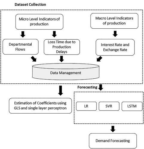
In this section, we discuss the dataset for the textile and apparel market. Furthermore, the traditional approaches to coefficient estimation in regression models and forecasting techniques are presented in detail. In the first step, we discuss the models of coefficient estimations such as GLS and the single-layer perceptron model. In the second step, we apply linear regression, SVR, and LSTM models to forecast the demand for textile apparel. Three evaluation matrices will be used for the comparison of forecasting results. These are mean squared error (MSE), mean absolute error (MAE) and root mean squared error (RMSE). The proposed methodology for the demand estimation is presented in Figure 1.

Figure 1. A proposed methodology for demand estimation of textile apparel.

3.1. Data

We used the daily production data of a textile firm. The data covered the nine months from May 3, 2021, to January 25, 2022. For micro-level parameters, we considered the data for different departments of the production process. These departments are stitching, washing, and packing. Moreover, we also used the time lost during production procedures due to absenteeism, cutting and handling delays, operator unavailability, and countless other reasons. We calculated the total lost time in minutes daily. To capture the influence of macro-level parameters, we applied the daily exchange, interest rates, and combined fabric export products worldwide. Table 2 lists the dataset details used for demand estimation and forecasting. Lost minutes due to production delays and departmental flows are micro-level or endogenous indicators, whereas interest and exchange rates are macro-level or exogenous indicators.

Table 2. Dataset Details.

Firm	Micro-level Indicators	Macro-level Indicators
Fabrics company	Lost minutes, Departments (Stitching, washing, finishing, and packing)	Interest rate and Exchange rate

Note: Duration of data: May 2021 to January 2022

3.2. Coefficient estimation models

In this section, we discuss the models we used to estimate coefficients. These models include GLS and single-layer perceptron models.

3.2.1. GLS model

This model estimates coefficients when the time-series dataset has autocorrelation. In such a case, the error term has a strong correlation with its lag value. If the problem of autocorrelation exists in the data set, then LR provides biased coefficient estimates. Therefore, the GLS model is used because it resolves the problem of autocorrelation. For the calculation of coefficients, we used Equation (1): (1) $D={\beta }_0+{\beta }_{1}LM+{\beta }_{2}I+{\beta }_{3}E+e_t$(1) In the above equation (1), D represents the demand of the textile industry, which is a dependent variable; LM is a microeconomic variable, namely lost minutes during production; and I and E represent the interest and exchange rates, respectively. These variables are treated as independent variables while the ${\beta }_0$ is the constant term. Moreover, when the dataset variance changes over time, the LR results become biased. Therefore, it is necessary to address this problem before estimating the coefficients. In the GLS approach, Equation (1) is divided by the variance to make it independent of time. Later on, the final equation is estimated to calculate the coefficients.

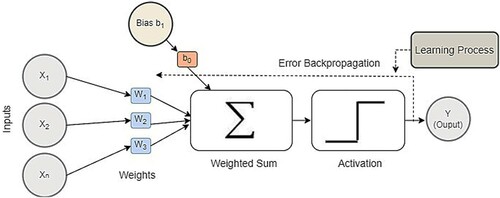
2.2.2. Single-layer perceptron model

This research employs the NN approach for an LR problem. The term "LR problem" refers to the problem set in which the relationship between dependent and independent variables is modelled. In contrast, the artificial neural network (ANN), inspired by the structure of the human brain, is a very efficient approach for designing a predictive model. The ANN architecture is made up of units, or nodes, and connections between them. Each unit conveys some information to the network. It first takes a vector of inputs as $X=(x_1,x_2,x_3)$ and uses a mathematical function to generate a predictive model. More precisely, $x_1$ shows the loss minutes, $x_2$ shows interest rate, and $x_3$represents the exchange rate in our model. In the next stage, it starts learning by fine-tuning the weights of connections among neurons, followed by measuring the model error. This error denotes the difference between the output of the predicted model and the actual values. This process is repeated for a set number of epochs to find a model with an error near zero. The ANN can model any real-world problem because it is self-adaptive. The ANN is divided into single-layer and multilayer NNs. We used a single-layer network consisting of only one input and one output layer to model the regression problem. A model was designed to take inputs of independent variables as a set of $X$ and learn by finding the best weights such that the value of the dependent variable and model outputs are nearly equal. Consider the simple LR function given in Equation (2): (2) $y=w_0+w_1{x}_1+w_2{x}_2+w_3{x}_3\dots w_n{x}_n$(2) In the above equation (2(2) $y=w_0+w_1{x}_1+w_2{x}_2+w_3{x}_3\dots w_n{x}_n$(2) ), $x_1$,$x_2$, $x_3,$and $x_n$ are independent variables or features in the given input vector, i.e., in our case these are micro and macro-economic indicators which include departmental flows, loss time due to production days, exchange rates, and interest rate, whereas $w_1$, $w_2,w_3$, and $w_n$ are the predictive model's coefficients and weights, or these micro and macroeconomic indicators, and $w_0$ is the bias term. The architecture consists of two layers: an input and an output layer. The number of units in the input layer equals the total number of independent variables, and one unit is in the output layer. Direct connections exist between every input and output unit along with the associated weights, as illustrated in Figure 2. The NN optimises these weights with the Adam optimiser iteratively (Kingma and Ba 2014). For different parameters, this algorithm calculates the individual learning rates. Moreover, to adapt to the learning rates, the first and second moments of the gradient are also calculated for each coefficient or weight of the model. The expected value of a random variable is defined as the moment of the variable, as indicated in Equation (3(3) $m=E[X^n]$(3) ): (3) $m=E[X^n]$(3) This random variable represents the loss function of the NN. Furthermore, when one iteration ends, the weights or coefficients of the LR model are updated based on the weight update rule given in equation (4(4) $W_n=W_{n-1}-\eta {\displaystyle \frac{{\hat{m}}_t}{\sqrt{\hat{v}t}+\epsilon }}$(4) ) for all weights (i.e., $w_0$,$w_1$, $w_2$, $w_3$, and $w_n$) that are associated with each micro and macro-economic indicator. (4) $W_n=W_{n-1}-\eta {\displaystyle \frac{{\hat{m}}_t}{\sqrt{\hat{v}t}+\epsilon }}$(4) In the above equation, $W_{n-1}$ is the value of the old weight associated with any micro-macroeconomic indicators; $\eta$ is the step size, and the values of ${\hat{m}}_t$ and $\hat{v}t$, which represent the moments and variance, respectively, are calculated using equations (5(5) ${\hat{m}}_t={\displaystyle \frac{m_t}{1-{\beta }_1^t},}$(5) ) and (6(6) ${\hat{v}}_t={\displaystyle \frac{v_t}{1-{\beta }_2^t},}$(6) ): (5) ${\hat{m}}_t={\displaystyle \frac{m_t}{1-{\beta }_1^t},}$(5) (6) ${\hat{v}}_t={\displaystyle \frac{v_t}{1-{\beta }_2^t},}$(6) where ${\beta }_1$ and ${\beta }_2$ are hyperparameters in Equations (5(5) ${\hat{m}}_t={\displaystyle \frac{m_t}{1-{\beta }_1^t},}$(5) ) and (6(6) ${\hat{v}}_t={\displaystyle \frac{v_t}{1-{\beta }_2^t},}$(6) ), whereas Equations (7(7) $m_t={\beta }_1{m}_{t-1}+(1-{\beta }_1)g_t,$(7) ) and (8(8) $v_t={\beta }_2{m}_{t-2}+(1-{\beta }_2)g_t^2$(8) ) are used for the calculation of $m_t$ and $v_t$: (7) $m_t={\beta }_1{m}_{t-1}+(1-{\beta }_1)g_t,$(7) (8) $v_t={\beta }_2{m}_{t-2}+(1-{\beta }_2)g_t^2$(8) The first moment is the mean $m_t$, whereas the second moment is the variance$v_t$. Furthermore, after the model converges and determines the best coefficients by updating the weights individually in every iteration, the weights or coefficients are extracted and stored, as depicted in Figure 2. The loss function, which is optimised, is the mean squared error function and can be defined as follows: $MSE={\displaystyle \frac{1}{n}\sum _{i=1}^n(Y_i-{\hat{Y}}_i{)}^2}$In Equation (9(10) $y={\alpha }_0+{\alpha }_1{X}_1+{\alpha }_2{X}_2+{\alpha }_3{X}_3\dots {\alpha }_k{X}_k+e$(10) ), n is the total number of instances in the data of daily production of a textile firm; $Y_i$ represents the actual value of the dependent variable. i.e., daily packed; and ${\hat{Y}}_i$ denotes the predicted value of the dependent variable, e.g., through LR, SVR, and LSTM. In the next stage, for unseen data, the stored coefficients are loaded and multiplied by the corresponding dependent variables to obtain the required value for dependent variables. Figure 2 illustrates the stepwise procedure of the single-layer perceptron model.

Figure 2. Single-layer perceptron.

2.3. Forecasting models

This section presents the details of the models we use to forecast production in textile apparel. These models include the LR, SVR, and LSTM models.

2.3.1. Linear regression

(10) $y={\alpha }_0+{\alpha }_1{X}_1+{\alpha }_2{X}_2+{\alpha }_3{X}_3\dots {\alpha }_k{X}_k+e$(10) In this research study, we employed a multiple LR model for demand forecasting. It has been observed from the research study of Nunno et al. (Nunno 2014) that regression models are accurate approaches with financial time series data, e.g., support vector regression and linear regression. For its strength and simplicity, the linear model is the most extensively used of all. In the current context, we used a multiple LR model for demand forecasting. Equation 1(1) $D={\beta }_0+{\beta }_{1}LM+{\beta }_{2}I+{\beta }_{3}E+e_t$(1) 0 forecasts the daily production of textile apparel, where Y denotes the daily production, whereas X_1, X_2, and X₃ represent loss minutes, interest rate, and exchange rate.

In the above equation (10(11) $D=(X_i,Y_i),1\le i\le N$(11) ), ${\alpha }_1,{\alpha }_2,{\alpha }_3$ represent the slope coefficients LM, I, and E. If there is a single unit change in LM, it will result in ${\alpha }_1$ a unit change in demand. Similarly, a unit change in interest rate causes ${\alpha }_2$units change in demand ${\alpha }_3$shows that when the exchange rate changes by 1 unit then demand changes by ${\alpha }_3$ units. These slope coefficients are calculated by minimising the error term e.

2.3.2. Support vector regression

The SVR follows the theory of statistical learning (Klein and Datta 2018), using machine learning algorithms to control structural risks. A modified version of SVR is preferred for forecasting (Guan et al. 2018). More precisely, a mapping between input spaces to real numbers is estimated in the problem of regression through SVR by giving the premise of training examples. In our case, these training examples are the daily production data for a textile firm. In support vector regression, the straight line is optimised so that it fits on data known as a hyperplane. This hyperplane fits the daily packed value, which is the required output. Contrary to the SVM, which is used for classification, the SVR that is used for regression finds the hyperplane that acts as a decision boundary to predict the continuous variable of daily packed. The data samples that are nearest to this hyperplane are called the support vectors. These are used to draw the needed curve that depicts the SVR model's projected outcome. The optimal fit curve in SVR is the hyperplane with the greatest set of data samples. Contrary to other regression models such as LR, in which errors between the actual and predicted values of daily packed variables are reduced, the SVR seeks to fit the optimal line over a certain range. Time-series data are assumed as follows: (11) $D=(X_i,Y_i),1\le i\le N$(11) In the above equation (11(12) $F(X_i)=WT\phi (X_i)+b$(12) ), $X_i$ denotes the variables which include LM, I, and E with m elements, and y_i represents the output data, or demand. The following regression function is relevant in this case: (12) $F(X_i)=WT\phi (X_i)+b$(12) In the above equation (12(13) $Min{\displaystyle \frac{1}{2}||W|{|}^2+C\sum _{i=1}^N({\epsilon }_i+{\epsilon }_{i^{\ast }})}$(13) ), $W$ represents the weight vector associated with these indicators, $b$ indicates the bias, and $\phi (X_i)$ maps the input vector $X$ to a higher dimensional feature space. The following optimisation function is solved for $W$ and$b$: (13) $Min{\displaystyle \frac{1}{2}||W|{|}^2+C\sum _{i=1}^N({\epsilon }_i+{\epsilon }_{i^{\ast }})}$(13) Subject to $y_i-W^T(\mathrm{\varnothing }(x))-b\le \xi +{\epsilon }_i$ ${\mathrm{W}}^{\mathrm{T}}(\mathrm{\varnothing }(\mathrm{x}))+\mathrm{b}-{\mathrm{y}}_{\mathrm{i}}\le \xi +{\epsilon }_{{\mathrm{i}}^{\ast }}$ ${\epsilon }_i,{\epsilon }_{i^{\ast }}\ge 0$

In the above equation (13(16) $y_i=f(X_i)=\sum _{i=1}^N((a_i-a_{i^{\ast }}))K(X_i,X_j)+b$(16) ), $C$ is a parameter that presents a positive trade-off between model simplicity, and generalizability, and it also aids in reducing data overfitting, and ${\epsilon }_i$ and ${\epsilon }_{i^{\ast }}$are slack variables measuring the error cost. Kernel functions are used for nonlinear datasets to map the original space to a higher dimensional feature space where an LR model can be built. The final form of the SVR function is as follows: (16) $y_i=f(X_i)=\sum _{i=1}^N((a_i-a_{i^{\ast }}))K(X_i,X_j)+b$(16) In the above equation (16(19) $RMSE=\sqrt{{\displaystyle \frac{1}{n}\sum _{i=1}^n{(Y_i-{\hat{Y}}_i)}^2}}$(19) ), $a_i$ and $a_{i^{\ast }}$ are Lagrange multipliers. The commonly used kernel function is the radial basis function with a width of σ: (17) $K(X_i,X_j)=exp(-{||X_i-X_j||}^2/2{\sigma }^2)$(17)

2.3.3. Long short-term memory method

In traditional NNs, all inputs and outputs are independent. However, in some cases, data are in a time series. Therefore, researchers have addressed this problem by introducing recurrent NNs (RNNs), which use hidden layers to remember hidden layers. The RNNs comprise an input, a hidden layer, and an output. The input layer provides input, and the hidden layer activates and provides the output through the output layer. It is calculated based on the hidden state and input provided by the previous timestamp of micro and macro indicators: (18) $H(T)=F((UX(T)+WH(T)+WH(T-1))$(18) In the above equation (18), $F$ represents a nonlinear transformation, $X(T)$ is the input at time $T$, and $H(T)$ denotes the state of the hidden layer at time $T$. In addition, RNNs have an input of hidden networks constrained by the weight matrix $U$, which is hidden, to output recurrent connections constrained by the weight matrix $V$ and loop recurrent connections constrained by the weight matrix $W$. All of the weights $(U,V,andW)$ are shared during that time. Further, $O(T)$ indicates the network output at the time stamp. Moreover, RNNs exhibit the strength of memorising significant information about the inputs, making them suitable for time-series forecasting. However, LSTM captures long-term dependency, which is difficult for RNNs, to capture and provides better predictions based on current information. The LSTM contains a long memory cell and three controllers called gates, which are the input, output, and forget gates. The function of the input gate is to determine what new information must be stored in the cell state. It works for the current input information from the previous time and filters out information about insignificant variables. The forget gate detects information that is no longer vital in the unit state and determines the forget vector. Finally, the output gate determines the output. We used the mean squared error (MSE), root mean squared error (RMSE), and mean absolute error (MAE) as evaluation matrices: (19) $RMSE=\sqrt{{\displaystyle \frac{1}{n}\sum _{i=1}^n{(Y_i-{\hat{Y}}_i)}^2}}$(19) (20) $MAE={\displaystyle \frac{1}{n}\sum _{i=1}^n|Y_i-{\hat{Y}}_i|}$(20) In the above equations (19) and (20), the $Y_i$ is the actual value, i.e., daily packed while ${\hat{Y}}_i$ is the predicted value by the model SVR, LSTM, and LR where $n$ is the total number of instances in the test set.

3. Results and discussions

In this section, we present the results along with a theoretical discussion. More precisely, in the first section, we first discuss the results of coefficient estimation, and later on, we discuss the results of the forecasting model.

3.1. Descriptive statistics

In Table 3, we present the descriptive statistics of all the model parameters, including micro-level (firm-level) and macro-level demand parameters. There are a total of seven micro-level parameters and three macro-level parameters. The mean and median value of departmental flows ranged from 57,000–59,500, except for the holding department, where the mean and median were 718 and 200, respectively. The mean and median of lost time were 205,559 and 160,181, respectively.

Table 3. Descriptive Statistics.

Micro-level demand parameters		Mean	Median	SD	Jarque–Bera Test	Observation
	Finishing	57,482	58,702	10,257.4	323.20*	209
	Daily packing	58,237	59,497	10,050	438.34*	209
	Holding	718	200	1,277.4	533.72*	209
	OK holding	58,208	59,461	9,808.3	533.72*	209
	Washing	58,428	59,431	96,065	107.41*	209
	Stitching	6,305	6,480	10,337	1135*	209
	Finishing to packing	58,220	59,491	10,060.2	437.87*	209
	Lost time	205,559	160,181	130,112	2066.97*	209
Macro-level demand parameters	Exchange rate	166.35	167.50	8.22	15.36*	209
	Interest rate	8.06	7.445	1.094	57.51*	209

* denotes significance at 1%.

¹For detection of autocorrelation in the data set, we have applied the LM test and Durbon Watson test and found them significant. Therefore, we applied the GLS model for coefficient estimation. Results of these tests can be provided if required.

More precisely, the standard deviations of the finishing variable are the highest among all variables, indicating that there are a lot of fluctuations in the values of this variable. However, if the statistics of the macro-level parameters are observed, then lost time has the highest standard deviation, while the interest rate standard deviation is very small, i.e., 1.094. In addition, the total number of observations for both macro-and microeconomic factors is 209, respectively. The Jarque-Bera test statistics for all variables were highly significant, confirming that nonlinearity is a common problem with time-series data (Jarque and Bera 1980)¹.

3.2. Unit root test

In time-series data, an inbuilt unit root problem exists (nonstationary). In this case, the mean and variance of the data series are dependent on time. If a unit root problem exists, the estimation results are inaccurate. Several tests investigate the unit root problem, such as the augmented Dickey-Fuller (ADF) test commonly used in the literature (Cheung and Lai 1995; Li et al. 2017; Lopez 1997). We used the ADF unit root test to investigate the time dependency of the mean and variance. This test considers the null of unit root vs. the alternative of no unit root. The unit root test results for stationarity are reported in Table 4. All datasets of micro-level parameters, excluding lost time, were stationary at the level. However, macro-level parameters (i.e. interest and exchange rates) were stationary at the first difference.

Table 4. Augmented Dickey-Fuller (ADF) Unit Root Test.

Departments	ADF test stat At level At 1st difference		Critical value at 5%	Stationary
Finishing	−7.721*		−2.889	At level
Daily packing	−8.361*		−2.889	At level
Holding	−5.947*		At Level	At level
OK holding	−8.365*		−2.889	At level
Washing	−8.037*		−2.889	At level
Stitching	−10.883*		−2.889	At level
Finishing to packing	−8.396*		−2.889	At level
Lost time	−2.496	−11.996**	−2.889	At 1st difference
Exchange rate	−1.137	−14.817**	−2.889	At 1st difference
Interest rate	−0.359	−18.456**	−2.889	At 1st difference

* and ** signal significance at 5% and 1%, respectively.

3.3. Coefficient estimation using the GLS and single-layer perceptron model

We used Equation (1(1) $D={\beta }_0+{\beta }_{1}LM+{\beta }_{2}I+{\beta }_{3}E+e_t$(1) ) for the estimation of coefficients. Table 5 presents the results of the GLS and single-layer perceptron model. The estimated coefficients of individual indicators are mentioned in the table followed by their respective t-stats in the parenthesis. The results of GLS indicate that the coefficient of lost minutes, ${\beta }_1$, is −0.05 and is significant at the 5% level; thus, a unit increase in lost minutes causes a 0.05-unit production decline. The coefficient of the interest rate, ${\beta }_2$, is positive but insignificant. The value of ${\beta }_3$ is 772.25, which is highly significant at the 1% significance level.

Table 5. Estimation of Coefficients using GLS and the Single-Layer Perceptron Model.

Model	Coefficients
	Constant ${\mathit{\beta }}_0$	Lost minutes ${\mathit{\beta }}_1$	Interest rate ${\mathit{\beta }}_2$	Exchange rate ${\mathit{\beta }}_3$
GLS	−76.23*** (−4.772)	−0.05** (−2.086)	512.05 (0.536)	772.25*** (6.203)
Single-Layer Perceptron	0.535** (2.564)	−0.136*** (−3.689)	0.1356 (1.356)	0.224*** (9.456)

*, **, and *** show significance at 10%, 5%, and 1%, respectively.

Therefore, if the exchange rate increases by 1 unit, the textile apparel production increases by 772.25 units, confirming that an increase in the exchange rate causes textile apparel exports to increase. Lost time has a significantly negative influence on exports. This means that any interruption in production reduces output and, as a result, market demand. The results of the single-layer perceptron model reveal that lost minutes have a significantly negative influence on production because its coefficient is −0.136, which is significant at the 1% level. In addition, ${\beta }_3$ is significant at the 1% level; thus, the local currency depreciation increases foreign demand, resulting in exports. This outcome is because the targeted firm exports all of its output. When the exchange rate appreciates, it causes domestic products to become cheaper for foreign consumers, which ultimately leads to an increase in demand. Therefore, sales (exports) of textile apparel increase because of the decrease in their relative prices. Our findings show that both the techniques complement each other. The overall findings of coefficient estimation show that textile production has remained insensitive toward interest rates. Furthermore, our findings of the single layer perceptron model show the evidence that the significance of the coefficients has increased from 5% to 1% in the case of exchange rate and loss minutes. The reason behind this improvement in the significance of individual parameters is the better performance of the neural network models.

3.4. Forecasting results

This section presents the results for both experiments, which were executed in Python and evaluated using the Mean Absolute Error (MAE), Mean Square Error (MSE), and Root Mean Square Error (RMSE). The parameters of the LSTM included a learning rate of 0.001 with the weight optimiser Adam and the loss function MSE with 100 epochs. The network has an input layer, a hidden layer with four LSTM blocks, or neurons, and an output layer with one neuron to predict a single value. The batch size was set to 1. The ARIMA model parameters include a lag value set to 5 for auto-regression, a different order of 1, and a moving average of 0.

3.4.1. Forecasting results with endogenous-level factors

This section presents demand forecasting results considering only endogenous level parameters as inputs. We also present the results using micro and macro-level parameters as inputs. We applied LR, SVR, and LSTM models to forecast the daily demand for textile apparel. Table 6 presents the demand forecasting results using only endogenous (micro/firm)-level inputs. Table 6's columns represent the model employed, while the rows represent the MAE, MSE, and RMSE values. LR has the lowest MSE value, whereas LSTM has the highest MSE value. Similarly, SVR obtained the second highest values for MSE, MAE, and RMSE. These inputs include the processes of stitching, washing, and finishing and the lost time based on production delays. The estimated evaluation matrices are MAE, MSE, and RMSE. We used three forecasting models: LR, SVR, and LSTM. The evaluation matrices indicate that LR provides the best results.

Table 6. Demand Forecasting based on Micro- or Firm-Level Parameters.

Evaluation matrix	Forecasting models
	LR	SVR	LSTM
MAE	0.0027	0.054	0.054
MSE	0.0000	0.002	0.005
RMSE	0.004	0.049	0.07

Figure 3 illustrates the spread of forecasted values of daily packing production using LR. We also present the spread of the actual values. Forecasting was done using micro- (endogenous) or firm-level inputs. The micro-level inputs included department flow data and lost time due to production delays. The blue line in Figure 3 indicates the actual value of daily packed while the orange line indicates the predicted values of daily packed from the LR algorithm. The graph indicates that the LR model produces such exact results that the difference between the two lines appears minor. Subsequently, Figure 4 displays the spread of forecasted values of daily packing production using the SVR model. Forecasting was done using micro- (endogenous) or firm-level inputs.

Figure 3. Graph of forecasted and actual values using linear regression (LR).

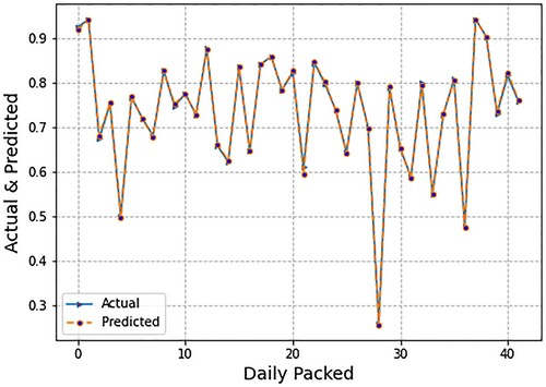
Figure 4. Graph of forecasted and actual values using support vector regression (SVR).

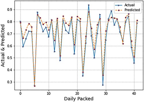
The micro-level inputs include department flow data and lost time due to production delays. We also present the spread of the actual values and predicted values. To be more specific, the blue line indicates the actual values of daily packed; however, the orange line indicates the predicted values of daily packed. If the comparison is made with LR, then the difference between actual and predicted lines, i.e., error, is higher in SVR. The orange line does not perfectly fit the blue line. Following, Figure 5 depicts the spread of forecasted values of daily packing production using the LSTM model. The forecasting was conducted based on micro (endogenous) or firm-level inputs. The micro-level inputs included department flow data and lost time due to production delays. In this case, we also present the spread of the actual values and predicted values. It is observed from Figure 5, that the results of LSTM are less than LR and SVM, i.e., the orange line does not perfectly fit the blue line, which are actual values of daily production. One might reason that fewer results with LSTM in comparison with LR and SVR is that deep learning models need more data to be effectively trained. Since we have fewer data points, the results are likewise fewer. In addition, Figure 6 illustrates the spread of loss minimisation using LSTM. We display epochs on the x-axis and the loss per epoch on the y-axis. This loss spread was plotted using only micro- or firm-level parameters as inputs. More precisely, the blue lines indicate the loss of validation data while the red lines indicate the loss of training data. Table 7 presents the demand forecasting results based on micro- or firm-level and macro (exogenous) inputs.

Figure 5. Graph of forecasted and actual values using long short-term memory (LSTM).

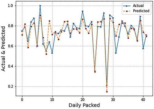
Figure 6. Graph of loss minimisation using long short-term memory (LSTM).

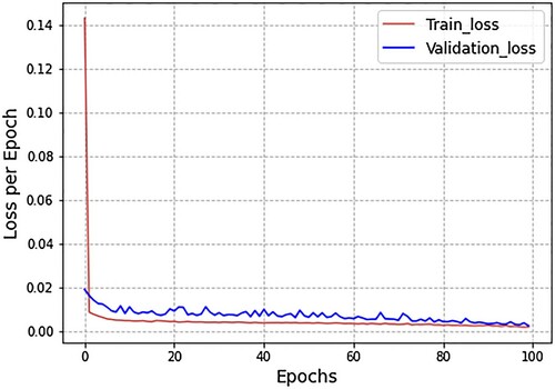
Table 7. Demand Forecasting based on Micro- and Macro-level Parameters.

Evaluation matrix	Forecasting model
	LR	SVR	LSTM
MAE	0.003	0.0411	0.048
MSE	0.000	0.002	0.004
RMSE	0.005	0.045	0.068

The columns of Table 7 indicate the model used, while the rows are the values of MAE, MSE, and RMSE. The lowest MSE value is achieved by LR, while LSTM shows a high value of MSE. Similarly, SVR achieved the second-highest values in terms of MSE, MAE, as well as RMSE. The micro-level inputs included the processes of stitching, washing, finishing, and packing and the lost time based on delays. Macro-level inputs include the daily exchange and interest rates. The estimated evaluation matrices were MAE, MSE, and RMSE. We used three forecasting models: LR, SVR, and LSTM. It is evident from the evaluation matrices that LR provides the best results. However, the results of SVR and LSTM significantly improved when macro-level indicators were incorporated as inputs in forecasting models. The overall accuracy of the SVR and LSTM improved by approximately 10% and 15%, respectively.

3.4.2. Forecasting results with both endogenous and exogenous-level factors

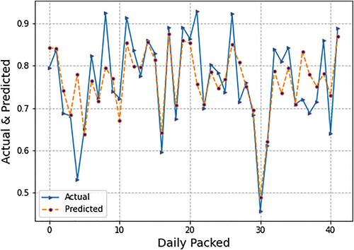
In the previous experiment, we only used micro- (endogenous) or firm-level inputs. In this second experimental design, however, we used both micro- (endogenous) or firm-level inputs and macro-level (exogenous) factors. For this experimental setting, Figure 7 depicts the spread of forecasted values of daily packing production using LR. Forecasting was done using micro- (endogenous) or firm-level inputs as well as macro- (exogenous) factors. Micro-level inputs include department flow data and lost time due to production delays, whereas macro-level indicators include the exchange (PKR/USD) and interest rates. We also present the spread of the actual values and predicted values. Figure 7 shows that LR produces very accurate results, just as it did in previous experimental designs that used only micro-(endogenous) or firm-level inputs. Subsequently, Figure 8 presents the spread of forecasted values of daily packing production using SVR. Forecasting was done using micro- (endogenous) or firm-level inputs as well as macro- (exogenous) factors. Micro-level inputs include department flow data and lost time due to production delays, whereas macro-level indicators include the exchange (PKR/USD) and interest rates.

Figure 7. Graph of forecasted and actual values using linear regression (LR).

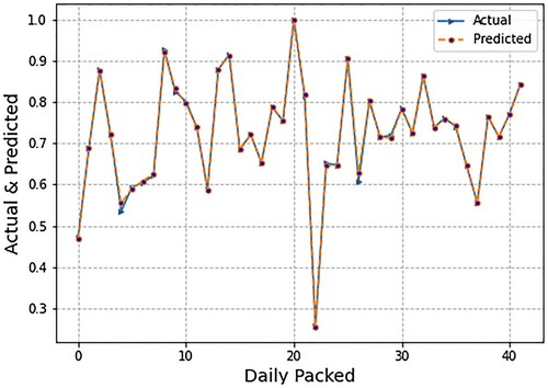
Figure 8. Graph of forecasted and actual values using support vector regression (SVR).

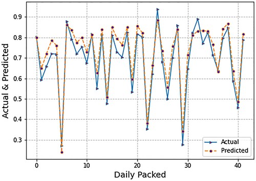
In Figure 8, the blue line shows the actual values of daily production while the orange line indicates the predicted values. The error through the SVR algorithm is higher than the simple LR algorithm. Figure 9 depicts the spread of forecasted values of daily packing production using LSTM. We also present the spread of the actual values. Forecasting was done using micro- (endogenous) or firm-level inputs as well as macro- (exogenous) factors. Micro-level inputs include department flow data and lost time due to production delays, whereas macro-level indicators include the exchange (PKR/USD) and interest rates. Due to the limited number of training data points, the results of LSTM are less than those of LR and SVM, i.e., the orange line does not precisely fit the blue line, which is the actual value of daily production.

Figure 9. Graph of forecasted and actual values using long short-term memory (LSTM).

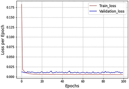
In addition, Figure 10 illustrates the spread of loss minimisation using LSTM, with the epochs on the x-axis and loss per epoch on the y-axis. This loss spread was plotted using micro and macro-level indicators as inputs. The blue line in Figure 10 shows the results of loss values on validation data, while the red lines demonstrate the epoch by epoch loss values on training data.

Figure 10. Graph of loss minimisation using long short-term memory (LSTM).

3.5. Theoretical contribution

Recently, demand forecasting has become a crucial matter in SCM. Researchers have used different models to forecast demand patterns for various industries. The textile industry is a sector that seeks the significant attention of researchers for demand forecasting. Traditional econometric approaches have commonly been used in demand forecasting. Existing research has primarily used endogenous input factors for demand forecasting. However, in the world of open economies, the macroeconomic environment also serves as a crucial parameter in demand forecasting. Therefore, this study used endogenous and exogenous factors as inputs for demand forecasting. In this context, exchange and interest rates were used as exogenous factors. For demand forecasting, these factors were combined with endogenous factors such as departmental flows and lost time. For the textile apparel firm's daily production, we used time-series data. Since the firm exports the whole lot of its production, we used micro and macro-level indicators for the demand forecasting. We applied the advanced machine learning models of SVR and LSTM, which provide more accurate results than traditional econometric approaches. In order to calculate the impact of individual parameters, we calculated the coefficients along with the respective t-stats. Our results indicate that textile apparel exporting firms are quite sensitive to the production delays, which ultimately cause the exports to decline. Furthermore, it is evident from our findings that firms exporting textile apparel are also quite sensitive to macroeconomic variation, especially the exchange rate. In this context, the present research study sheds light on the crucial factors that must be considered while production processes and market demand estimation are.

3.6. Implications for practice

Since globalisation and open economies have begun, export industries have been very sensitive to macroeconomic movements. The textile and apparel industries account for the largest export volume in the textile sector. The demand for textile apparel depends on multiple factors based on micro and macro-level dimensions. We combined endogenous and exogenous factors to forecast the textile apparel demand for the textile industry in Pakistan. The results indicate that, among micro-level indicators, lost minutes due to production delays significantly negatively influence textile apparel production. Furthermore, the exchange rate appreciation increases the exports of textile apparel. The forecasting results reveal that the SVR model performs better when macro-level indicators are used as inputs. The overall accuracy of SVR and LSTM improves by approximately 10% and 15%, respectively. In contrast, LR provides better results based on all evaluation metrics, and the accuracy of the LR does not improve when macro-level indicators are added to the forecasting model. In this context, the SCM process should decrease lost minutes (i.e., production delays because of countless internal factors). Furthermore, policymakers should consider macroeconomic economic factors while developing international trade policies, especially the exchange rate, as it affects the production and demand of the textile exporting sector. Moreover, new parameters should be included in endogenous (micro) and exogenous (macro) factors for demand forecasting. A comparison of different industries can also provide a better direction for future research.

Demand forecasting is an important part of SCM; therefore, this research encourages the business community to consider micro and macro-level parameters, such as the production process and macroeconomic indicators. For policymakers, it is of prime importance to consider and manage the exchange rate and other macroeconomic variables, as the production and demand of the textile sector are very sensitive to these highly volatile exogenous explanatory variables.

5. Conclusion

In this study, we focused on forecasting the production of the textile and apparel industries. The time-series dataset for a textile clothing company was used. The dataset covered the period from May 3, 2021, to January 25, 2022. A combined forecasting model is applied to estimate the coefficients of explanatory variables (i.e. micro and macro-level parameters). We have used GLS and single-layer perceptron models. It is observed from the findings that micro (endogenous) and macro-level (exogenous) parameters were significant, and the coefficient of lost time was negatively significant at the 5% level. Moreover, the company exports all of its production; thus, the exchange rate is a crucial factor in determining its demand. The results provide evidence that, among macro-level parameters, exchange rate appreciation increases the exports of textile apparel. In addition, we have employed the LR, SVR, and LSTM models to forecast the production of textile apparel. The results indicate that LR provides a better forecast than SVR and LSTM. However, unlike SVR and LSTM, the forecasting accuracy of the LR did not improve when macro-level indicators were incorporated into the forecasting system. In demand forecasting, the biggest limitation is the availability of time-series datasets, which are rarely available. The present study faced the same problem. In line with this limitation of dataset unavailability, future research needs to be conducted based on extensive datasets. Moreover, additional macro-level (exogenous) parameters should be incorporated into the forecasting models.

Data availability statement

The data can be made available by contacting the corresponding author.

Disclosure statement

No potential conflict of interest was reported by the author(s).

Additional information

Funding

This paper was supported by Korea Institute for Advancement of Technology (KIAT) grant funded by the Korea Government (MOTIE) (P0008703, The Competency Development Programme for Industry Specialist).

References

- Ahmad, S., S. Miskon, R. Alabdan, and I. Tlili. 2020. “Towards Sustainable Textile and Apparel Industry: Exploring the Role of Business Intelligence Systems in the era of Industry 4.0.” Sustainability 12 (7): 2632.
- Altman, E. I., G. Marco, and F. Varetto. 1994. “Corporate Distress Diagnosis: Comparisons Using Linear Discriminant Analysis and Neural Networks (the Italian Experience).” Journal of Banking & Finance 18 (3): 505–529.
- Armstrong, J. S. 2001. Principles of Forecasting: A Handbook for Researchers and Practitioners (Vol. 30). New York: Springer.
- Box, G. E., G. M. Jenkins, G. C. Reinsel, and G. M. Ljung. 2015. Time Series Analysis: Forecasting and Control. Hoboken, NJ: John Wiley & Sons.
- Brieman, L., J. Friedman, R. Olshen, and C. Stone. 1984. Classification and Regression Trees. Belmont, CA: Wadsworth.
- Brown, R. G. 2004. Smoothing, Forecasting and Prediction of Discrete Time Series. Chelmsford, MA: Courier Corporation.
- Bukhari, M., K. B. Bajwa, S. Gillani, M. Maqsood, M. Y. Durrani, I. Mehmood, H. Ugail, and S. Rho. 2021. “An Efficient Gait Recognition Method for Known and Unknown Covariate Conditions.” IEEE Access 9: 6465–6477.
- Cheung, Y.-W., and K. S. Lai. 1995. “Lag Order and Critical Values of the Augmented Dickey–Fuller Test.” Journal of Business & Economic Statistics 13 (3): 277–280.
- Chmura, C. 1987. “The Effect of Exchange Rate Variation on US Textile and Apparel Imports.” FRB Richmond Economic Review 73 (3): 17–23.
- Croston, J. D. 1972. “Forecasting and Stock Control for Intermittent Demands.” Journal of the Operational Research Society 23 (3): 289–303.
- Fisher, M., and K. Rajaram. 2000. “Accurate Retail Testing of Fashion Merchandise: Methodology and Application.” Marketing Science 19 (3): 266–278.
- Greco, S., B. Matarazzo, and R. Slowinski. 2001. “Rough Sets Theory for Multicriteria Decision Analysis.” European Journal of Operational Research 129 (1): 1–47.
- Guan, H., Z. Dai, A. Zhao, and J. He. 2018. “A Novel Stock Forecasting Model Based on High-Order-Fuzzy-Fluctuation Trends and Back Propagation Neural Network.” PLoS ONE 13 (2): e0192366.
- Güven, İ., & Şimşir, F. 2020. “Demand Forecasting with Color Parameter in Retail Apparel Industry Using Artificial Neural Networks (ANN) and Support Vector Machines (SVM) Methods.” Computers & Industrial Engineering 147: 106678.
- Haq, A. U., A. Zeb, Z. Lei, and D. Zhang. 2021. “Forecasting Daily Stock Trend Using Multi-Filter Feature Selection and Deep Learning.” Expert Systems with Applications 168: 114444.
- Harrison, P. J., and C. Stevens. 1971. “A Bayesian Approach to Short-Term Forecasting.” Journal of the Operational Research Society 22 (4): 341–362.
- Ilyas, W., M. Noor, and M. Bukhari. 2021. “An Efficient Emotion Recognition Frameworks for Affective Computing.” The Journal of Contents Computing 3 (1): 251–267.
- Jantarakolica, T., and P. Chalermsook. 2012. “Thai Export Under Exchange Rate Volatility: A Case Study of Textile and Garment Products.” Procedia - Social and Behavioral Sciences 40: 751–755.
- Jarque, C. M., and A. K. Bera. 1980. “Efficient Tests for Normality, Homoscedasticity and Serial Independence of Regression Residuals.” Economics Letters 6 (3): 255–259.
- Karpavičius, S., and F. Yu. 2017. “The Impact of Interest Rates on Firms’ Financing Policies.” Journal of Corporate Finance 45: 262–293.
- Kingma, D. P., and J. Ba. 2014. “Adam: A Method for Stochastic Optimization.” arXiv Preprint ArXiv 1412: 6980.
- Klein, M. D., and G. S. Datta. 2018. “Statistical Disclosure Control via Sufficiency Under the Multiple Linear Regression Model.” Journal of Statistical Theory and Practice 12 (1): 100–110.
- Kuo, R., and K. Xue. 1999. “Fuzzy Neural Networks with Application to Sales Forecasting.” Fuzzy Sets and Systems 108 (2): 123–143.
- Langley, P., W. Iba, and K. Thomas. 1992. “An analysis of Bayesian classifier.” Proceedings of the Tenth National Conference on Artificial Intelligence. San Jose, CA, July 12–16, 1992, pp. 223–228.
- Lee, K. C., and S. B. Oh. 1996. “An Intelligent Approach to Time Series Identification by a Neural Network-Driven Decision Tree Classifier.” Decision Support Systems 17 (3): 183–197.
- Li, B., J. Zhang, Y. He, and Y. Wang. 2017. “Short-term Load-Forecasting Method Based on Wavelet Decomposition with Second-Order Gray Neural Network Model Combined with ADF Test.” IEEE Access 5: 16324–16331.
- Lin, J. C.-W., Y. Djenouri, and G. Srivastava. 2021a. “Efficient Closed High-Utility Pattern Fusion Model in Large-Scale Databases.” Information Fusion 76: 122–132.
- Lin, J. C.-W., Y. Djenouri, G. Srivastava, and P. Fourier-Viger. 2022. “Efficient Evolutionary Computation Model of Closed High-Utility Itemset Mining.” Applied Intelligence 52: 10604–10616.
- Lin, J. C.-W., Y. Djenouri, G. Srivastava, U. Yun, and P. Fournier-Viger. 2021b. “A Predictive GA-Based Model for Closed High-Utility Itemset Mining.” Applied Soft Computing 108: 107422.
- Lopez, J. H. 1997. “The Power of the ADF Test.” Economics Letters 57 (1): 5–10.
- Lorente-Leyva, Leandro L., M. M. E. Alemany, Diego H. Peluffo-Ordóñez, and Roberth A. Araujo. 2021a. “Demand Forecasting for Textile Products Using Statistical Analysis and Machine Learning Algorithms.” Paper presented at the Intelligent Information and Database Systems, Cham.
- Lorente-Leyva, L. L., M. Alemany, D. H. Peluffo-Ordóñez, and R. A. Araujo. 2021b. “Demand Forecasting for Textile Products Using Statistical Analysis and Machine Learning Algorithms.” Paper presented at the Asian Conference on Intelligent Information and Database systems.
- Lorente-Leyva, L. L., M. M. E. Alemany, D. H. Peluffo-Ordóñez, and I. D. Herrera-Granda. 2020. “A Comparison of Machine Learning and Classical Demand Forecasting Methods: A Case Study of Ecuadorian Textile Industry.” Paper Presented at the Machine Learning, Optimization, and Data Science, Cham.
- Maqsood, H., M. Maqsood, S. Yasmin, I. Mehmood, J. Moon, and S. Rho. 2022. “Analyzing the Stock Exchange Markets of EU Nations: A Case Study of Brexit Social Media Sentiment.” Systems 10 (2): 24.
- Medina, H., M. Peña, L. Siguenza-Guzman, and R. Guamán. 2021. “Demand Forecasting for Textile Products Using Machine Learning Methods.” Paper presented at the International Conference on applied technologies.
- Müller, W., and E. Wiederhold. 2002. “Applying Decision Tree Methodology for Rules Extraction Under Cognitive Constraints.” European Journal of Operational Research 136 (2): 282–289.
- Murray, P. W., B. Agard, and M. A. Barajas. 2018. “Forecast of Individual Customer’s Demand from a Large and Noisy Dataset.” Computers & Industrial Engineering 118: 33–43.
- Nunno, L. 2014. Stock Market Price Prediction Using Linear and Polynomial Regression Models. Albuquerque, NM, USA: Computer Science Department, University of New Mexico.
- Papalexopoulos, A. D., and T. C. Hesterberg. 1990. “A Regression-Based Approach to Short-Term System Load Forecasting.” IEEE Transactions on Power Systems 5 (4): 1535–1547.
- Pegels, C. C. 1969. “Exponential Forecasting: Some New Variations.” Management Science 15 (5): 311–315.
- Prak, D., and R. Teunter. 2019. “A General Method for Addressing Forecasting Uncertainty in Inventory Models.” International Journal of Forecasting 35 (1): 224–238.
- Prak, D., R. Teunter, and A. Syntetos. 2017. “On the Calculation of Safety Stocks When Demand is Forecasted.” European Journal of Operational Research 256 (2): 454–461.
- Shao, Y., J. C.-W. Lin, G. Srivastava, D. Guo, H. Zhang, H. Yi, and A. Jolfaei. 2021. “Multi-Objective Neural Evolutionary Algorithm for Combinatorial Optimization Problems.” IEEE Transactions on Neural Networks and Learning Systems 1–11.
- Spedding, T., and K. Chan. 2000. “Forecasting Demand and Inventory Management Using Bayesian Time Series.” Integrated Manufacturing Systems 11 (5): 331–339.
- Syntetos, A. 2001. Forecasting of intermittent demand. London: Brunel University Uxbridge.
- Syntetos, A. A., and J. E. Boylan. 2005. “The Accuracy of Intermittent Demand Estimates.” International Journal of Forecasting 21 (2): 303–314.
- Teunter, R. H., A. A. Syntetos, and M. Z. Babai. 2011. “Intermittent Demand: Linking Forecasting to Inventory Obsolescence.” European Journal of Operational Research 214 (3): 606–615.
- Thomassey, S., and A. Fiordaliso. 2006. “A Hybrid Sales Forecasting System Based on Clustering and Decision Trees.” Decision Support Systems 42 (1): 408–421.
- Van Donselaar, K. H., V. Gaur, T. Van Woensel, R. A. Broekmeulen, and J. C. Fransoo. 2010. “Ordering Behavior in Retail Stores and Implications for Automated Replenishment.” Management Science 56 (5): 766–784.
- West, M., and J. Harrison. 2006. Bayesian forecasting and dynamic models. New York: Springer Science & Business Media.
- West, M., P. J. Harrison, and H. S. Migon. 1985. “Dynamic Generalized Linear Models and Bayesian Forecasting.” Journal of the American Statistical Association 80 (389): 73–83.
- Willemain, T. R., C. N. Smart, J. H. Shockor, and P. A. DeSautels. 1994. “Forecasting Intermittent Demand in Manufacturing: A Comparative Evaluation of Croston's Method.” International Journal of Forecasting 10 (4): 529–538.
- Yasmin, S., M. Y. Durrani, S. Gillani, M. Bukhari, M. Maqsood, and M. Zghaibeh. 2022. “Small Obstacles Detection on Roads Scenes Using Semantic Segmentation for the Safe Navigation of Autonomous Vehicles.” Journal of Electronic Imaging 31 (6): 061806.
- Yelland, P. M. 2010. “Bayesian Forecasting of Parts Demand.” International Journal of Forecasting 26 (2): 374–396.
- Zadeh, L. A. (1996). Advances in Fuzzy Systems — Applications and Theory, Fuzzy Logic, and Fuzzy Systems: Selected Papers by Lotfi A Zadeh, edited by George J. Klir and Bo Yuan, 796-804. Singapore: World Scientific.