A deep learning model to detect foggy images for vision enhancement

ABSTRACT

Fog limits meteorological visibility, posing a significant danger to road safety. Poor visibility is considered as a significant contributor to road accidents in foggy weather conditions. Regardless, image defogging techniques can only work with foggy images. In a real-time system, however, defogging foggy images becomes difficult if they are not identified as foggy or clear. Because we cannot rely on human vision to distinguish between foggy and clear pictures, we need a robust model that classifies the input image as foggy or clear based on some features. This paper proposes a robust Deep Learning (DL) model based on Convolutional Neural Network (CNN) for classifying the input as foggy and clear. The proposed Deep Neural Network (DNN) architecture is efficient and precise enough to classify images as foggy or clear, with a training time complexity of $\mathcal{O}\left(n^2\right)$ and a prediction time complexity of $\mathcal{O}\left(n\right)$. The experimental results reveal promising results in both qualitative and quantitative assessments. The model has an accuracy of 94.8%, precision of 91.8%, recall of 75.8% and F1 score of 80.3% when evaluated on the SOTS dataset, indicating that it might be utilized to mitigate the safety risk in vision enhancement systems.

KEYWORDS:

• Classification
• clear
• DNN
• dropout
• foggy

1. Introduction

Many external video monitoring, driver assistance and optical remote sensing systems are currently configured to function in good weather and visibility conditions; however, one of the critical conditions which influence the likelihood of a road accident is poor visibility caused due to some atmospheric catastrophe. In foggy or hazy weather, poor visibility is frequent, and it can significantly affect the precision and efficiency of vision enhancement systems. It is exceedingly difficult for a motorist to detect visible cars, warnings and objects coming from the other direction in poor visibility conditions, which increases the possibility of an accident. Correspondingly, when a train runs in foggy weather, the locomotive pilot cannot see the signals correctly, making the surveillance strenuous. Therefore, some of the researchers have introduced some classical dehazing algorithms [1–3] to enhance the visibility of driver assistance systems to reduce the safety risk. In a level of co-occurrence, 3287 people worldwide die from traffic accidents every day on average, resulting in an annual number of deaths of over 1.4 million, while 20–50 million people sustain injuries. Every year, more than 11,000 lives are lost in road accidents due to fog, and almost 24,000 individuals are wounded due to such accidents, contributing to about 16% of all road accidents [4–6].

Fog is usually formed when the aerosol particles become saturated, resulting in a drastic fall in visibility to less than 1 km and thereby the contrast and colour of an image are degraded due to fog, which significantly influences the functioning of external imaging systems [7–11]. Therefore, it is of the utmost importance to remove fog from images and thus classify them into foggy and clear for the proper functioning of vision enhancement systems. Narasimhan and Nayar present a model based on Dichromatic Atmospheric Dispersion to analyse the variability of the colour of the scene in [7]. Since then, researchers have started focusing on analysing foggy images, developing diverse models and algorithms for removing fog and restoring the ground truth image. Several image enhancement techniques like histogram-based [12], Dark Channel Prior (DCP) based [13–15] and saturation-based [16, 17] methods are employed to remove haze from the degraded image effectively. In recent years, researchers [1–3, 18–21] have developed some classical dehazing algorithms using Deep Learning (DL) which has achieved a remarkable dehazing effect for driver assistance systems. However, since there was no classification done among those images, the majority of researchers have classified the input image as foggy or clear based on subjective judgment. For the input image, it frequently appears that the input is clearer than the output or the fog is so little there is no need of defogging. As a result, issues like contrast saturation that is too strong and a challenge to remove dense fog may arise. Therefore, a reliable framework for classifying foggy images is required, on which various defogging methods may then be used.

In this paper, we introduce a robust DL model based on CNN to classify an input image into foggy or clear. In the proposed end-to-end DNN architecture, we have used Leaky Rectified Linear Unit (ReLU) to activate the network layers to subdue dying ReLU. We have divided the input image into three colour components: red, green and blue. Each of these colour components is trained and validated over 80% data of a benchmark dataset, Synthetic Objective Testing Set (SOTS) [22] and tested over the rest 20 %. Both quantitative and qualitative evaluations of the proposed model reveal promising results for classifying the input images as foggy or clear.

After the introduction, we organize the rest of the paper as follows: Section 2 describes the prevailing research in the classification of foggy images and clear images along with the research gap and contribution. Section 3 presents the proposed method based on a robust DL framework, while Section 4 highlights the experimental results and discussions. Finally, Section 5 concludes the research work.

2. Literature survey

It is broadly acknowledged that foggy images reduce the efficacy of vision enhancement algorithms. For the dispersion of light in the surroundings, the contrast and colour of the image do degrade [18, 31, 32] which significantly impacts the stable functioning of outdoor imaging systems, and thus it is of utmost importance to classify the foggy and non-foggy images. Table 1 depicts several significant pieces of research in the domain of classification of foggy and non-foggy images in a nutshell.

Table 1. Considerable research for classifying foggy and clear images.

Authors	Method used	Features	Constraints	Accuracy
Yu et al. [23]	Eigenvalues; SVM	Can handle multiple images at a time	Considers random images	Not provided
Pavlic et al. [24]	Spectral Features; Linear Classifier	Global descriptors are used; Uses a large dataset	Does not perform well in high contrast; Generates horizontal gradients in dark regions	95.35%
Mao et al. [25]	Haze Degree Estimation	No need of entering manual input constraint	Can not be applied to a monochrome light source; Uses a very small dataset	Not provided
Thakur et al. [26]	Visibility Index	Handles both batch and real-time processing	Can not classify noisy images; A small dataset is used	92%
Wan et al. [27]	Gaussian Mixture Model	Can be performed on outdoor images	Picks up random images from the internet	89.8%
Shrivastava et al. [28]	19 Classification Techniques	Fits for both cluster and steady planning structure	Uses a small dataset; Can not deal well with noisy images	89.06%
Hao et al. [29]	Brightness Optimization; Colour Correction	Works with noisy images; Can be used both in the daytime and nighttime scenes	Does not consider haze level in small areas	89%
Chincholkar et al. [30]	CNN	Visibility distance can be computed	Uses a small dataset	82%

In the beginning, hand-designed characteristics like [33, 34] were mostly employed for classifying hazy and clear photos. A haze degree estimate tool is created to automatically identify foggy images at various haze degrees [25]. To assess an image's haziness and further categorize the photos, an unique technique is introduced in the reference [26]. The classifications of hazy and non-hazy photos are established using the parameters Lowest Pixel Intensity, Average, Sample Variance and Highest Pixel Intensity. However, [23] retrieves three distinct eigenvalues: the image's visibility, image contrast and dark channel intensity. To assess the input class, Support Vector Machine (SVM) is then used.

Using Gabor filters in a range of scales, frequencies and orientations, [24] identifies clear images that are global and facilitates the usage of image descriptors and a classification process. However, to determine whether an image is foggy or clear, 19 classification techniques have been proposed in [28]. The classifier system is trained using various differences between clear and foggy pictures, which are represented by the five parameters that make up the area: standard deviation, mean, lowest intensity and peak intensity.

In [27], a technique is proposed that the fog-degraded weather conditions can be classified into different categories, e.g. fog, thick fog and thick fog. The feature vectors used to build the training model are utilized to extract the contrast and characteristics of hazy pictures. However, in [29], the authors establish a technique to deal with noise with the help of a Butterworth filter, supported by a Recurrent Convolutional Neural Network (RCNN) for the identification of haze levels. As a follow-up, [30] aims to develop a method for predicting the viewable area of foggy pictures based on factors including luminance, intensity, variance and image brightness using a basic CNN.

2.1. Research gaps

After conducting an in-depth examination of cutting-edge approaches, we identified the following research gaps:

• Most of the existing approaches [23–30] do not use a benchmark dataset for experimentation purpose. These approaches often predict the input image as fog-degraded or clear based on a visual evaluation only, which may raise concerns about the efficacy of the algorithm.

• The algorithms are not capable of efficiently dealing with noise.

• The authors have not actively participated in calculating the computational time complexity.

• It is not apparent that the algorithm's performance is measured using any parameter other than the accuracy score. Even in several studies [24, 26–30], the accuracy rate is quite low.

2.2. Contributions

We made a contribution by modifying the present to attain improved accuracy after analysing the research gap. The following are some of this study's beneficial aspects:

• We have considered two subsets: SOTS and Hybrid Subjective Testing Set (HSTS) from a benchmark dataset, REalistic Single Image DEhazing (RESIDE) [22] for training and testing the performance of the end-to-end DNN.

• In our proposed DNN, we have considered noise as nothing but a distortion in the signal. Sometimes, it can be caused by the sound of the shutter of the camera. The proposed DNN architecture has several two-dimensional max-pooling and average pooling layers extensively, which results in a uniform distribution of noise in the entire image. Therefore, the proposed model successfully classifies the image even if such small noise is present.

• The training time complexity of the proposed algorithm is $\mathcal{O}\left(n^2\right)$, and the predicting time complexity is linear, i.e. $\mathcal{O}\left(n\right)$.

• We tested the model to use on a benchmark dataset and obtained a decent accuracy rate of 94%. Additionally, we took precision, recall, and F1 score into account while evaluating the performance of the suggested model in addition to the single standard measure (accuracy).

3. Proposed method

Our work introduces a simple and efficient end-to-end DNN architecture based on classical CNN to classify foggy and clear images. When compared to previously proposed state-of-the-art classification algorithms, the pre-processing needed for the proposed DNN is much lower.

We consider two subsets, HSTS [22] and the indoor set of Synthetic Objective Testing Set (SOTS) indoor [22] from an openly accessible major benchmark dataset RESIDE [22] for training and testing the model, and also for evaluating the performance of the model on untrained data. We have randomly taken 80% of data from the indoor subset of SOTS [22] to train and validate the model. Let us denote this amount of data with D. We use the rest of 20% data from this subset to test the model's performance. We have taken another 80% data from D to train the model, and the rest of the data from D is used for validation. Each image of the dataset is divided into three components, viz. red, green and blue. We have resized the input images in shape $28\times 28$ and then re-scaled it between 0 and 1. Then we slice the image matrix into three channels producing three arrays of shape $28\times 28\times 1$ each, and then each of these matrices is fed to the network as input data.

3.1. Network architecture

The concerned network works with 2D CNN. The pooling operation mentioned has a pool size $(2,2)$. For each layer, filters (F) in the following order are considered: 32,64, 128 and 256. Linear activation is used to activate each layer. In other words, by passing the necessary parameters, namely, the reshaped colour channel, we were able to generate an instance of the Convolution 2D function having receptive field (K) of the size of $4\times 4$ and the skip value or the stride is one. There are also three 2D average pooling layers and one 2D max-pooling layer, all of which have a pooling size of $2\times 2$ and no padding. In the network, the max-pooling operation is used to identify the darker and brighter pixels of the input image. On the other hand, we use three average pooling layers to smoothen the data. We understand that everything is dependent on the amount of computer RAM used to create the DNN. The generated layers can be visualized using the summary function, which also calculates the total number of parameters in the final model as well as the parameters for each layer, weights and biases. These layers have a significant impact on the learning parameters and classification accuracy.

The activation function Rectified Linear Unit (ReLU) is used in a leaky way so that the deactivation by ReLU [35] does not occur. The value of is $\alpha =0.1$ in LeakyReLU, while activating the layers of the proposed DNN. The usage of ReLU is widely spread, especially in CNN, as it sets the activation threshold to a minimum(0). But when we use this revolutionary layer of ReLU during training, the layers can be fragile and die. This is because when some data with a large gradient flows through the ReLU neurons, it can cause the weight to update so that the neuron will never be activated at any point. All of the neurons in the preceding superficial layer provide information to each neuron in the following two-dimensional average pooling layer. This layer's activation method is softmax activation. It is trained over ten epochs, and thus the data for each colour component is trained and validated. We depict the algorithm of the proposed model in Section 3.3.

3.2. Training and testing of the proposed DNN

Training and testing of our proposed model make the process more straightforward when we add the data to arrays, train_X, test_X respectively. As the name suggests, it is the trained and test dataset. We then add the data label in the arrays named train_Y, test_Y and reshape the arrays named train_X, test_X to (−1, 28, 28, 1) format and change their datatype from int8 to float32. Thus, when re-scaled, the negative values are also considered, making the network flexible. The class labels are now being converted hot encoding vector that is a numeric array. The input of this encoding is a prediction class which denotes that discrete categorical features take on the values. One-hot encoding is used to encrypt these labels, resulting in a binary column for each category. Usually, the one-hot encoding yields a sparse matrix. In one-hot encryption, the categorical data is converted into a numeric vector. The categorical data is to be converted into single hot encryption to work for multilabel classification. One column for each category or class can be generated with ease. Only one of these columns might be given the value 1 for each sample. The one-hot encoding, which is nothing more than a straightforward row vector with a dimension of $1\times 2$ for each input class, is what is referred to as ‘encoding '.

The vector is entirely composed of zeros, with the exception of the class it represents, which has a value of 1. To ensure good generalization of the model, the training data is divided into two segments: one for training and one for model validation. Currently, 20% of the remaining D data has been verified throughout the dataset, and 80% of the D data has been trained. As a consequence, the model checks the data that it was not exposed to during training, improving the test results and assisting in reducing the overfitting problem.

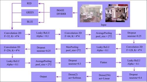
The recommended DNN can efficiently learn the issue and overfit the training dataset given its size. Hence, the final model cannot generalize well that results in poor performance when the model is evaluated, and we depict the performance in Section 4. The workflow diagram for the proposed model is depicted in Figure 1 when the problem persists. We avoid the problem with the help of a method of regularization, dropout. The training procedure could get noisier as a result, pushing the nodes inside a layer to probabilistically accept varying degrees of accountability for the inputs. It implies that it could eliminate circumstances when network tiers work together to fix mistakes made by earlier layers, enhancing the model as a consequence. The intriguing result of dropout is that it encourages the network to learn a sparse representation by duplicating a layer's sparse activation. During execution, it just randomly turns off a portion of the neurons, which lowers the amount of dependency on training. This layer randomly changes the input units to 0 with a frequency of rate r at each stage of the training process. When an input is not set to 0, it is scaled up by $\frac{1}{(1-r)}$ such that the sum of all the inputs stays constant. When we employ dropout to address the issue of data overfitting, we show the workflow diagram of the model in Figure 2. It is important to note that dropout only functions when the training parameter is set to ‘True,’ which prevents any data from being deleted during inference. We compare our observations when dropout is used versus when it is not in the following section.

Figure 1. The network architecture of the proposed DNN without dropout layer.

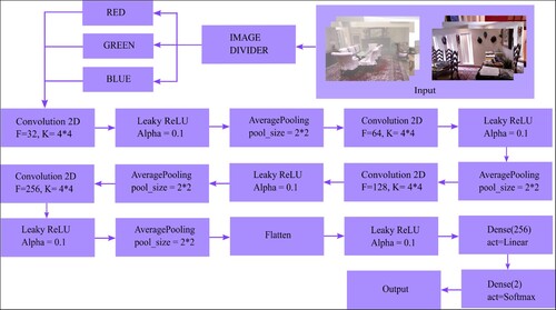
Figure 2. The network architecture of the proposed DNN after solving the issue of data overfitting.

3.3. Algorithm

Algorithm 1 shows the different steps of the proposed approach:

Algorithm 1

Algorithm of the proposed method

Require: Input Image Dataset

Ensure: Classification Report

1: Divide all the components of RGB image

2: for each-component do

3:   Resize data in $28,28$

4:   Add the train data in an array, $train\mathrm{\_}X$

5:   Add the test data in an array $test\mathrm{\_}X$

6:   Add the label of the data in $train\mathrm{\_}Y$ and $test\mathrm{\_}Y$ array

7:   Reshape the array $train\mathrm{\_}X$ and $test\mathrm{\_}X$ in $(-1,28,28,1)$

8:   Hot encode the $train\mathrm{\_}Y$ and $test\mathrm{\_}Y$ data

9:   Initialize a sequential model named "model"

10:  Add the following layers in the model.

11:  Conv2D: Filter: 32, Kernel: $4\times 4$, activation: linear

12:  LeakyReLU: alpha = 0.1

13:  AveragePooling2D: pool_size = $2\times 2$

14:  Conv2D: Filter: 64, Kernel: $4\times 4$, activation: linear

15:  LeakyReLU: alpha = 0.1

16:  AveragePooling2D: pool_size = $2\times 2$

17:  Conv2D: Filter: 128, Kernel: $4\times 4$, activation: linear

18:  LeakyReLU: alpha = 0.1

19:  AveragePooling2D: pool_size = $2\times 2$

20:  Conv2D: Filter: 256, Kernel: $4\times 4$, activation: linear

21:  LeakyReLU: alpha = 0.1

22:  AveragePooling2D: pool_size = $2\times 2$

23:  Flatten the model

24:  Dense: Filter 256, activation: linear

25:  LeakyReLU alpha = 0.1

26:  Dense: filter 2, activation= softmax

27:  Compile the model and fit it

28:  Run the model on train dataset by splitting it in ratio 8:2

29:  Initialize a sequential model named "model"

30:  Add the following layers in the model.

31:  Conv2D: Filter: 32, Kernel: $4\times 4$, activation: linear

32:  LeakyReLU: alpha = 0.1

33:  AveragePooling2D: pool_size = $2\times 2$

34:  Dropout: Percent 0.3

35:  Conv2D: Filter: 64, Kernel: $4\times 4$, activation: linear

36:  LeakyReLU: alpha = 0.1

37:  AveragePooling2D: pool_size = $2\times 2$

38:  Dropout: Percent 0.3

39:  Conv2D: Filter: 128, Kernel: $4\times 4$, activation: linear

40:  LeakyReLU: alpha = 0.1

41:  AveragePooling2D: poolsize = $2\times 2$

42:  Dropout : Percent 0.3

43:  Conv2D: Filter: 256, Kernel: $4\times 4$, activation: linear

44:  LeakyReLU: alpha = 0.1

45:  AveragePooling2D: pool_size = $2\times 2$

46:  Dropout : Percent 0.3

47:  Flatten the model

48:  Dense: Filter 256, activation: linear

49:  LeakyReLU: alpha = 0.1

50:  Dense: filter 2, activation= softmax

51:  Compile the model and fit it

52:  Run the model on train dataset by splitting it in ratio 8:2

53:  Fit the model and run the model on testing dataset

54:  Predict the classes and generate classification report.

55: end for

4. Discussion of experimental results

In this section, we discuss the experiments performed and the results obtained for our proposed DNN model to classify foggy and clear images.

We have performed the experiments on the Red Geen Blue (RGB) images from the indoor set of SOTS [22], and afterwards, we deploy the results of the performance of our proposed model on an untrained subset of RESIDE [22], HSTS [22]. The experiments are performed on a laptop with having Ubuntu 18.04.5 LTS operating system, with Intel Pentium(R) CPU N3710 1.60 GHz processor and 4 GB RAM. The experimentations are simulated with Python 3.6.13.

4.1. Optimization, training and testing of the proposed DNN

We have considered the red, green and blue components of each image from the dataset separately. The adam optimizer is used to find the global minima of the loss function [36]. We provide a description of the environment hyper-parameters in Table 2 . The indoor set of SOTS [22] is then used to train and evaluate the proposed model. We tabulate the data components we have taken into account, which are the identical for all three of the colour components, in Table 3.

Table 2. Environment hyper-parameters.

Hyper-parameter	Value
LR	0.001
Decay of Weights	0.0001
Training Batch Size	64
Number of Epoch	10
Optimizer	Adam

Table 3. The data components used during experimentation of the model proposed.

	Value
Training data shape	(440, 28, 28)
Testing data shape	(110, 28, 28)
Total no. of outputs	2
Output classes	[0 1]

For all of the colour components, the total number of training parameters is $(650,754)$. There is no such existence of any untrained parameter. After testing the model on the remaining 20% of data, we conclude whether the image is foggy or not depending on the majority of foggy or clear colour channels.

4.1.1. Quantitative analysis of the model

The accuracy metric, which only accounts for the proportion of properly categorized data instances to all data instances, is by no means enough to evaluate the model's performance quantitatively. The real negative situations that the model retrieves can sometimes be overlooked. Therefore, we must assess the model's accuracy. A detailed representation is made of the genuine positive prediction %. When we desire the lowest possible false negative, we can compromise precision for recall. If we wanted to have as few false positives as feasible, we would compromise recall for precision. The problem of poor accuracy and high recall score so continues, requiring the creation of a metric that combines both of these measurements. An illustration of one of these metrics is the F1 score. When accuracy and recall are combined to produce the harmonic mean, commonly known as the F1 score, false positives and false negatives are also taken into account. As a result, it is advantageous if the data distribution is imbalanced. To evaluate each of the colour components, the weight distribution and classification report, which includes the accuracy, recall, and $F_1$ scores are used.

4.1.1.1 Problem of data overfitting

While performing the experiments for the proposed DNN, we have observed that the training dataset does overfit while validating the model and has avoided the problem of data overfitting with dropout. In the proposed DNN architecture, 0.25%, 0.25%, 0.25%, 0.4%, 0.3 % of neurons are consecutively dropped out to refer to the problem mentioned above of data overfitting.

Now, we deploy the confusion matrices in Table 4 for each of the colour components, viz. red, green and blue, when we do not use dropout and we tabulate the classification reports for each of the colour components in Table 5, when we do not use dropout. We use class 1 for denoting clear images, and 0 for foggy images.

Table 4. Confusion matrices for red, green and blue colour components when dropout is not used.

Red	Confusion Matrix	Output YES	Output NO
	True YES	98	0
	True NO	0	12
Green	Confusion Matrix	Output YES	Output NO
	True YES	98	0
	True NO	1	11
Blue	Confusion Matrix	Output YES	Output NO
	True YES	98	0
	True NO	1	11

Table 5. Classification reports of the colour components when dropout is not used.

Colour Component	Class Label	Precision	Recall	$F_1$ Score
Red	0	1.00	1.00	1.00
	1	1.00	1.00	1.00
Green	0	0.99	1.00	0.99
	1	1.00	0.92	0.96
Blue	0	0.99	1.00	0.99
	1	1.00	0.92	0.96

We, then tabulate the values for accuracy of each of the colour components in Table 6 when dropout is not used.

Table 6. Accuracy reports of the colour components when dropout is not used.

Red	Accuracy			1.00
	Macro Average	1.00	1.00	1.00
	Weighted Average	1.00	1.00	1.00
Green	Accuracy			0.99
	Macro Average	0.99	0.96	0.98
	Weighted Average	0.99	0.99	0.99
Blue	Accuracy			0.99
	MacroAverage	0.99	0.96	0.98
	WeightedAverage	0.99	0.99	0.99

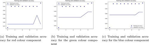
In continuation, in Figure 3, we plot the graphs for loss during training and validation. As the graphs for training and validation are not close to each other, the model is clearly overfitting. On the other hand, Figure 4 represents the accuracy during training and validation of the model.

Figure 3. Training and validation loss for the (a) red (b) blue and (c) green colour components when dropout is not used: (a) training and validation loss for the red colour component; (b) training and validation loss for the green colour component and (c) training and validation loss for the blue colour component.

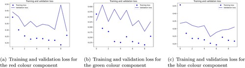
Figure 4. Training and validation accurcy for the (a) red (b) blue and (c) green colour components when dropout is not used: (a) training and validation accuracy for red colour component; (b) training and validation accuracy for the green colour component and (c) training and validation accuracy for the blue colour component.

4.1.1.2 The final model

From Tables 5 and 6, it is prominent that the training dataset is overfitted. This is why we employ dropout to avoid the problem of data overfitting. After optimization, we validate the model and tabulate the metrics of step loss, loss accuracy (accuracy), validation loss, and validation accuracy per epoch for all of the colour components in Table 7.

Table 7. Table for the values of step loss, accuracy, validation loss and validation accuracy for each of the colour components after using dropout.

Metric	Colour component	Epoch
		01	02	03	04	05	06	07	08	09	10
Step Loss	Red	0.4006	0.3013	0.2547	0.2294	0.2356	0.2333	0.2214	0.2199	0.1849	0.2589
	Green	0.3910	0.2639	0.2523	0.2169	0.1830	0.1281	0.1177	0.1266	0.0589	0.0525
	Blue	0.3988	0.2579	0.2580	0.2594	0.2232	0.1717	0.1191	0.1230	0.1442	0.1033
Accuracy	Red	0.9202	0.9202	0.9202	0.9202	0.9202	0.9202	0.9202	0.9259	0.9459	0.9259
	Green	0.8551	0.9148	0.9148	0.9148	0.9148	0.9517	0.9574	0.9716	0.9801	0.9830
	Blue	0.8722	0.9148	0.9148	0.9148	0.9148	0.9148	0.9602	0.9602	0.9545	0.9631
4pc Validation Loss	Red	0.4402	0.4038	0.3273	0.3680	0.3245	0.3448	0.3361	0.3361	0.4948	0.2908
	Green	0.2616	0.2431	0.2388	0.2329	0.1739	0.2301	0.2543	0.2536	0.2363	0.2412
	Blue	0.2572	0.2560	0.2517	0.2534	0.2394	0.2404	0.2686	0.1643	0.1491	0.2033
Validation Accuracy	Red	0.8750	0.8750	0.8750	0.8750	0.8750	0.8977	0.8977	0.9091	0.8977	0.9091
	Green	0.8909	0.8909	0.8909	0.8909	0.9359	0.9218	0.9359	0.9359	0.9359	0.9473
	Blue	0.9091	0.9091	0.9091	0.9091	0.9091	0.9218	0.9091	0.9218	0.9202	0.9561

We now tabulate the metrics we have used to quantify the performance of the proposed final model, in which we have dropped out several nodes from the layers. The classification accuracy for each colour component is based on the confusion matrix obtained. We set out the confusion matrix for each of the colour components in Table 8 and the classification report of each of the colour components of the final model in Table 9.

Table 8. Confusion matrices for red, green and blue components of the final model.

Red	Confusion Matrix	Output YES	Output NO
	True YES	98	0
	True NO	3	9
Green	Confusion Matrix	Output YES	Output NO
	True YES	98	0
	True NO	5	7
Blue	Confusion Matrix	Output YES	Output NO
	True YES	98	0
	True NO	8	4

Table 9. Classification reports of the colour components of the final model.

Colour Component	Class Label	Precision	Recall	F1 Score
Red	0	0.97	0.97	0.97
	1	0.67	0.67	0.67
Green	0	0.95	1.00	0.98
	1	1.00	0.58	0.74
Blue	0	0.92	1.00	0.96
	1	1.00	0.33	0.50

We hence get the accuracy of each of the colour components, viz. red, green and blue in Table 10. We sum up both of the accuracy and loss reports in Table 11. We have utilized categorical cross-entropy as the loss function, and it should be noted that the type of loss per epoch is provided for binary classification. To provide a more precise average value of a loss, we present loss as the product of actual loss and 100 in Table 11. We depict the graphs for training and validation loss for each of the colour components in Figure 5, followed by, Figure 6 which depicts the graphs for training and validation accuracy of each of the colour components.

Figure 5. Training and validation loss for the (a) red (b) blue and (c) green colour components of the final model: (a) training and validation loss for the red colour component; (b) training and validation loss for the green colour component and (c) training and validation loss for the blue colour component.

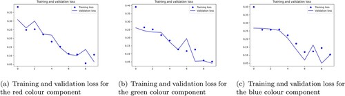
Figure 6. Training and validation accuracy for the (a) red (b) blue and (c) green colour components of the final model: (a) training and validation accuracy for the red colour component; (b) training and validation accuracy for the green colour component and (c) training and validation accuracy for the blue colour component.

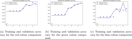
Table 10. Accuracy report for each of the colour components of the final model.

Red	Accuracy			0.94
	Macro Average	0.82	0.82	0.82
	Weighted Average	0.94	0.94	0.94
Green	Accuracy			0.95
	Macro Average	0.98	0.79	0.86
	Weighted Average	0.96	0.95	0.95
Blue	Accuracy			0.93
	Macro Average	0.96	0.67	0.73
	Weighted Average	0.93	0.93	0.91

Table 11. Overall accuracy and loss report of the final model.

Component	Validation		Testing
	Accuracy	Loss × 100	Accuracy	Loss × 100
Blue	91.7431	22.8344	93.5780	25.8716
Green	91.7431	23.6588	96.3303	18.8875
Red	92.6605	23.4250	94.4954	26.8286
Average	92.0489	23.3061	94.8012	23.8626

4.1.2. Qualitative analysis of the model

An aspect we have adapted to qualitatively evaluate the performance of the model proposed is to predict the classes based on the outputs of several state-of-the-art defogging techniques. We have chosen a subset of a major benchmark dataset RESIDE [22], HSTS [22] to perform the experiment. We have taken five images from HSTS [22] into consideration and defogged with the help of five prevailing defogging techniques, proposed by Li et al. [3], Sebastian et al. [37] and Ancuti et al. [38], Ngo et al. [39], Li et al. [40] and then classified the images with the help of the model proposed. The ground truth and foggy images were also considered for evaluating the performance of the classifier. As per the images seen in Figure 7, the ground truth images are classified as ‘CLEAR’. However, the image at position $(3,2)$ is classified as clear. This is because either of the two colour channels have classified the image as clear. We observe that the edges are not at all visible in the image at $(1,3),(1,5),(4,5),(4,6)$ and thus, it is labeled as ‘FOGGY’. The image at position $(1,6)$ is also classified as foggy as the contrast of the image is degraded after defogging. The edges are not at all properly visible since the image is not defogged properly. On the other hand, for the image at the position $(5,3)$, the brightness is affected, and the fog is not effectively removed. Hence, the classifier has classified the image as foggy when the class should be clear.

Figure 7. Classification of hazy and clear images on different outputs by different researchers: (a) clear images; (b) foggy images; (c) defogged by the method proposed by Li et al. [3]; (d) defogged by the method proposed by Sebastian et al. [37]; (e) defogged by the method proposed by Ancuti et al. [38]; (f) defogged by the method proposed by Ngo et al. [39]; (g) defogged by the method proposed by Li et al. [40].

For qualitatively analysing the performance of the proposed model with some existing classifiers, we have chosen random forest [41], polynomial SVM [42], sigmoid SVM [33], gaussian SVM [43] and implemented them separately. There is a rare implementation of other metrics, viz. F1 score, recall, and precision to evaluate the performance of these classifiers. It can be interpreted that random forest predicts based on the number of the prevailing models. There is a need to compile the model with the help of other agents to make random forests flexible and executable, thus taking more time. Although it performs poorly for linear models, polynomial SVM aids in learning non-linear models, and sigmoid SVM uses the $\tan \left(h\right)$ function. They can be used as a proxy for a neural network, but Softmax is far better than $\tan \left(h\right)$ in terms of multilabel classification. Euclidean distance is used by Gaussian SVM for classification, although occasionally they overfit the data. We have to extract several features like mean, standard deviation, and entropy for each classifier, which makes the process complex. From Table 12, we observe that the proposed model shows promising results than the existing classical machine learning classifiers in terms of accurately classifying the foggy images and the computational time complexity of the proposed method is low as there is no need of extraction of features. We analyse the efficiency of our model with several state-of-the-art classification models in Table 13. Several classifiers like VGG16 [44], ResNet50 [45], MKL-Based Model [46], Alex Net [47] have been considered and Alex Net [47] has performed the best amongst the four. Research of how network depth affects accuracy in a large-scale image recognition environment led to the creation of the first piece of network architecture, which is cited as [44]. ResNet50 [45] restructures the layers so that they are now learned residual functions with reference to the inputs of the layers rather than unreferenced functions. The third method, of Zhang et al. [46], extracts various weather features, learns dictionaries based on those features to better the performance of multiple weather classification and improve picture representation discrimination. The most recent state-of-the-art classifier, known as [47], has 650,000 neurons and 60 million parameters. It has five convolutional layers, some of which are followed by max-pooling layers, three fully connected layers, and a final 1000-way softmax. On the other hand, several prevailing techniques for foggy image classification can be found in [48–51] with the accuracies of 92%, 91.4%, 92.6% and 93%. However the accuracy of the proposed method is 94% when evaluated on SOTS dataset [22]. Kang et al. [48] present a deep learning-based weather image recognition framework by considering the three most common whether phenomena as haze, rain and snow. In contrast, Xiao et al. [50] describe a revolutionary deep convolutional neural network termed MeteCNN for classifying meteorological events. Wang et al. [49] suggest a lightweight model by stacking cutting-edge building components. They compile 6877 images of 11 different weather events into a database known as the weather phenomenon database. Finally, Satrasupalli et al. [51] developed a novel technique to estimate the transmission map based on a mean channel prior, which corresponds to the depth map. Before continuing with the dehazing, the researchers advised utilising a deep neural network to detect the hazy image (Table 14).

Table 12. Comparative analysis of some existing machine learning classifiers.

Classifier	Accuracy	Remarks
Random Forest	93%	High computaional complexity, features are needed to be extracted.
Linear SVM	89%	High computaional complexity, features are needed to be extracted.
Polynomial SVM	88%	High computaional complexity, features are needed to be extracted.
Sigmoid SVM	88%	High computaional complexity, features are needed to be extracted.
Gaussian SVM	89%	High computaional complexity, features are needed to be extracted.
Proposed Model	94%	Low computational complexity, no need to extract features

Table 13. Ablation study of the proposed architecture with some existing deep learning image classification model.

Model	Accuracy
VGG16 [44]	75.59%
ResNet50 [45]	49.28%
MKL-Based Model [46]	71.8%
Alex Net Based Model [47]	90.2%
Proposed Model	94%

Table 14. Comparative analysis of the proposed model with some existing deep learning techniques.

Model	Accuracy
Kang et al. [48]	92%
Wang et al. [49]	91.4%
Xiao et al. [50]	92.6%
Satrasupalli et al. [51]	93%
Proposed Model	94%

We have performed cross-validation for all of the three colour channels and have written the values of repeated K fold, time series split, and startified K fold cross validation in Table 15. We discuss the cross-validation methods herein.

Table 15. Cross validation score.

Colour component	Validation type	Accuracy
Red	Repeated K Fold	94.5%
	Time Series	90.2%
	Startified K Fold	94.8%
Green	Repeated K Fold	94.2%
	Time Series	88.4%
	Startified K Fold	91%
Blue	Repeated K Fold	95%
	Time Series	93%
	Startified K Fold	95.6%

4.1.3. Repeated k- fold cross validation

It is possible that the model performance estimate from k-fold cross-validation is noisy. This implies that each time the technique is done, the dataset can be divided into k-folds in a unique fashion. As a result, the performance score distribution can change, which will alter the mean estimate of the performance of the model. The degree to which the anticipated performance differs between k-fold cross-validation runs depends on both the model being used and the dataset. It may be difficult to determine which result should be compared and used as the ideal model to address the problem, making a noisy estimate of model performance irritating. One method to reduce noise in the anticipated model performance is to raise the k-value. While the variance will rise, this will reduce the bias in the estimated performance of the model, for instance, by more closely connecting the result to the specific dataset used for the evaluation. Using the k-fold cross-validation technique several times and then publishing the mean performance overall folds and repeats is an alternative approach. Commonly referred to as repeated k-fold cross-validation. We have obtained the accuracy of 94.5%, 94.2%, 95% for red, green, and blue channels for this kind of cross-validation.

4.1.4. Time series cross validation

Folds are produced via forward chaining for time series cross validation. The goal behind time series splits is to split the training set into two folds at each iteration, supposing that the validation set is always in front of the training set. Margin is introduced twice in order for it to work. The first one occurs between the training and validation folds to prevent the model from detecting lag values that are utilized twice–once as a regressor and again as a responder. Every iteration employs two folds to avoid the model memorising patterns from one iteration to the next. The accuracy values for the three colour channels are successively 90.2%, 88.4%, and 93%.

4.1.5. Startified K fold

A sampling strategy known as stratified sampling chooses the samples in the same proportion as they appear in the dataset. If a dataset, for example, comprises photographs that are 70% clear and 30% hazy, we would divide the dataset into these two groups and choose 70% of the sample from the clear group and 30% from the hazy group. Cross-validation makes sure that the training and test sets include the same amount of the important feature as the original dataset by using the stratified sampling technique. The cross-validation outcome, when applied to the target variable, is a close approximation of the generalization error. This method provides accuracy for the red, blue, and green colour channels of 84.8%, 91% and 95.6%, respectively.

4.2. The suggested model's computational time complexity

The most fundamental aspect of evaluating the performance of an algorithm is to determine the computational time complexity. In our proposed algorithm, we have used forward propagation to train the DNN and monitored loss as a checkpoint. Forward propagation is the inference phase of a feed-forward neural network. The approach for determining the asymptotic complexity of the forward propagation is similar to the procedure for determining the run-time complexity of multiplication between two matrices. The following is the feed-forward propagation algorithm: Initially, to propagate from layer a to layer b, we do (1) $S_j=W_{ba}\times Z_b$(1) where the activation function is $Z_b=f\left(S_b\right)$and $W_{ba}$ is the weight transfer from layer b to layer a. Including input and output layer if we have N layers, this will run N−1 times.

Now, for the proposed algorithm, the model without dropout has 17 layers, where a signifies the number of nodes from the input layer, b represents the second layer's number of nodes, c denotes the third layer's number of nodes, and so on. As there are 17 layers, we need 16 matrices to represent the weight between the matrices. Let us denote them by $W_{21},W_{32},W_{43}$ and so on. Thus $W_{ij}$ denotes the weight transfer from b to a, where $j,i\in [1,16]$.

If we have t training examples to propagate, from layer i to j, we do (2) $S_{bt}=W_{ba}\times Z_{at}$(2) and as this operation is a matrix multiplication operation, the complexity is $\mathcal{O}(b\ast a\ast t)$. We then apply the activation function (3) $Z_{bt}=f\left(S_{bt}\right)$(3) Thus, in total, we have (4) $\mathcal{O}(b\times a\times t+b\times t)=\mathcal{O}(b\times t\times (a+1\left)\right)=\mathcal{O}(b\times a\times t)$(4) In our proposed method, as we have used a data of shape $28\times 28$, the complexity will be reduced to $\mathcal{O}(j\times i)$.

The proposed DNN architecture uses the cross entropy-based softmax function as its activation function. Many neural networks convert the output of the last layer into class scores using a softmax function. The softmax function takes an N dimensional vector of scores and pushes the values into the range $[0,1]$ as represented by the function: (5) $f_j\left(z\right)=\frac{e^{z_j}}{\sum _{k=1}^N{e}^{z_k}}$(5) where $z_a$ is the ath vector.

During training, using datasets with particularly large output spaces might soon cause a computational bottleneck. This is the outcome of the last matrix multiplication in this model between the output weights, which are size $d\times K$ (K is the number of classes or output space), and the hidden states, which are size $B\times d$ (B is the batch size and d is the dimension for the hidden state). The difficulty of the other operations in the model is rapidly reduced when the output classes are large, and because the denominator relies on the sum of each vector, the complexity of softmax is $\mathcal{O}\mathcal{\left(}\mathcal{n}\mathcal{\right)}$.

Next, we use the concept of max-pooling to find out the maximum value from the pool and then redistribute it to the matrix. Let us say the pool size is $i\times j$ and the input shape is $m\times n$. So it will be pooling the maximum value $\frac{m\times n}{i\times j}$ times. Moreover, as the pool size is minimal, the searching can be done linearly. Furthermore, $m\times n>>i\times j$. therefore $\frac{m\times n}{i\times j}=m\times n$ and the time complexity for pooling layer is $\mathcal{O}\left(n^2\right)$

So the total complexity of the algorithm without dropout is $\mathcal{O}\left(n^2\right)$

Ensembles of neural networks with alternative model configurations have been shown to reduce data overfitting; nevertheless, training and maintaining several models adds to the computational cost. We have previously seen that the training dataset overfits when we do not use dropout. Undoubtedly dropout layer minimizes the problem, but it also uses additional time for this process. However, when it is compared with the total loss, the computational cost is negligible. Thus, the time complexity of the overall algorithm for training is $\mathcal{O}\left(n^2\right)$.

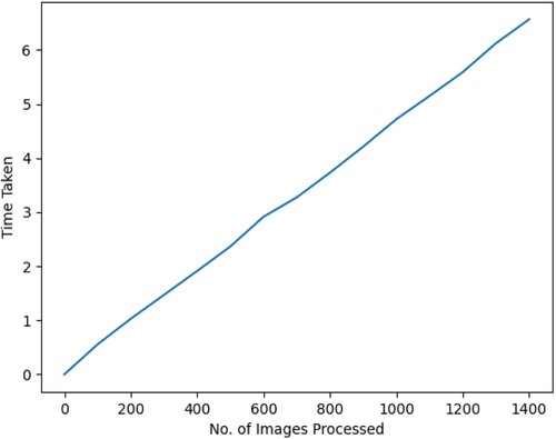
To determine the testing time complexity, we took one thousand and four hundred samples. The time taken to predict those samples in an interval of hundred is taken and plotted in Figure 8. The graph obtained is linear, and we can readily conclude that the testing complexity is $\mathcal{O}\left(n\right)$

Figure 8. Predicting time complexity for the method proposed.

5. Conclusion

Fog has a great impact on the transportation system and outdoor image surveillance systems, posing a danger to road safety risk. Despite the fact that the researchers [52–57] have developed a number of image defogging approaches, it can be difficult to defog foggy images in a real-time system if they are not correctly distinguished from clear ones. So that defogging is effective, it is necessary to create a reliable model that can separate the input image into foggy and clear. However, the focus of current image classification research is on training feed-forward CNNs with very big structures [58]. Hence, this paper proposes a DL model based on CNN for classifying the input image as foggy and clear. We first divide the input image into three colour components: red, green, and blue. We train and validate all of these colour channels over the SOTS indoor set [22]. We have transformed the categorical data into a one-hot numeric vector, which is further converted into a single hot encryption to be used for multilabel classification. We aim to further expand our work with fog depth classification to use an algorithm for multilabel classification instead of binary classification. Nevertheless, when we do not use dropout, we observe that the red colour component of the images overfits the training dataset, which is not desirable at all. We hence opt for a regularization technique, dropout, which is nothing but randomly dropping the nodes of several layers of the DNN architecture, to avoid the problem of data overfitting. On completion of training and testing, if either of the two colour channels is classified as foggy, the input is hence classified as foggy. The proposed model can be used for mitigating the road safety risk of commuters and motorists since it has achieved a good accuracy rate of 94%. On getting the dehazed outputs by several state-of-the-art methods, viz. Li et al. [3], Sebastian et al. [37], Ancuti et al. [38], Ngo et al. [39] and Li et al. [40], we classify the outputs into foggy and clear and compare the results with the ground truth, and hazy images from HSTS [22]. We tested the model on a dataset of real-world foggy photos: SOTS [22]. The experimental results show encouraging results, which pave the way for various computer vision-based applications.

Acknowledgments

We would like to thank the most esteemed anonymous reviewers for the helpful comments and suggestions.

Data availability

The data are available on request from the corresponding author.

Disclosure statement

No potential conflict of interest was reported by the author(s).

Additional information

Notes on contributors

Tannistha Pal

Tannistha Pal (Member, IEEE) received the Ph.D. degree in Computer Science & Engineering from Tripura University (A Central University), India in 2021. She is currently an Assistant Professor with the Department of Computer Science and Engineering, National Institute of Technology (NIT) at Agartala, India. She has published two patents and 20 publications in conference proceedings, book chapters and in reputed journals. Her research interests include image processing, deep learning, computer vision, pattern recognition and medical imaging.

Mritunjoy Halder

Mritunjoy Halder is a final year B. Tech student in the Dept. of Information Technology of Indian Institute of Engineering Science and Technology (IIEST), Shibpur, India. He has published papers in conferences and referred journals. He conducts his research activities in Image processing, robotics, artificial Intelligence and computer vision.

Sattwik Barua

Sattwik Barua (Student member, IEEE) is a final year B. Tech student in the Dept. of Computer science & Engineering of Indian Institute of Engineering Science and Technology (IIEST), Shibpur, India. He has published papers in referred journals and in conferences. His current research interests include image processing, embodied artificial intelligence, data science and multimedia.

References

- Cao Z, Qin Y, Jia L, et al. Haze removal of railway monitoring images using multi-scale residual network. IEEE Trans Intell Transp Syst. 2020;22(12):7460–7473.
- Liu Q, Qin Y, Xie Z, et al. An efficient residual-based method for railway image dehazing. Sensors. 2020;20(21):6204.
- Li B, Peng X, Wang Z, et al. Aod-net: all-in-one dehazing network. In: Proceedings of the IEEE International Conference on Computer Vision. 2017. p. 4770–4778.
- World Health Organization. Global status report on road safety 2015. Geneva, Switzerland: World Health Organization; 2015.
- Malik Y. Road accidents in india 2016. In: Ministry of Road Transport and Highways, Government of India, New Delhi (August 2017). 2017.
- World Health Organization. Violence and injury prevention and world health organization: Global status report on road safety 2018: Supporting a decade of action. 2018.
- Narasimhan SG, Nayar SK. Vision and the atmosphere. Int J Comput Vis. 2002;48(3):233–254.
- Krizhevsky A, Sutskever I, Hinton GE. Imagenet classification with deep convolutional neural networks. Adv Neural Inf Process Syst. 2012;25:1097–1105.
- Narasimhan SG. Models and algorithms for vision through the atmosphere. Columbia: Columbia University; 2004.
- Al-Zubaidy Y, Salam RA. Removal of atmospheric particles in poor visibility outdoor images. Telkomnika Indonesian J Electric Eng. 2013;11(8):4244–4250.
- Yu J, Wang Y, Zhou S. Haze removal algorithm using color attenuation prior and guided filter. In: Proceedings of the 3rd International Conference on Multimedia Systems and Signal Processing. 2018. p. 41–45.
- Gang D, Zhenyu L, Wei X, et al. Improved algorithm on haze removal based on dark channel prior and histogram specification. In: Proceedings of the 2nd International Conference on Innovation in Artificial Intelligence. 2018. p. 116–120.
- He K, Sun J, Tang X. Single image haze removal using dark channel prior. IEEE Trans Pattern Anal Mach Intell. 2010;33(12):2341–2353.
- Wang Y, Wu B. Improved single image dehazing using dark channel prior. In 2010 IEEE International Conference on Intelligent Computing and Intelligent Systems. Vol. 2. IEEE; 2010. p. 789–792.
- Xu H, Guo J, Liu Q, et al. Fast image dehazing using improved dark channel prior. In: 2012 IEEE International Conference on Information Science and Technology. IEEE; 2012. p. 663–667.
- Lu Z, Long B, Yang S. Saturation based iterative approach for single image dehazing. IEEE Signal Process Lett. 2020;27:665–669.
- Kim SE, Park TH, Eom IK. Fast single image dehazing using saturation based transmission map estimation. IEEE Trans Image Process. 2019;29:1985–1998.
- Han X-H, Sun Y, Chen Y-W. Residual component estimating cnn for image super-resolution. In: 2019 IEEE Fifth International Conference on Multimedia Big Data (BigMM). IEEE; 2019. p. 443–447.
- Sun W, Wang R. Fully convolutional networks for semantic segmentation of very high resolution remotely sensed images combined with dsm. IEEE Geosci Remote Sensing Lett. 2018;15(3):474–478.
- Wu F, Wang Z, Zhang Z, et al. Weakly semi-supervised deep learning for multi-label image annotation. IEEE Trans Big Data. 2015;1(3):109–122.
- Chaabani H, Kamoun F, Bargaoui H, et al. A neural network approach to visibility range estimation under foggy weather conditions. Procedia Comput Sci. 2017;113:466–471.
- Li B, Ren W, Fu D, et al. Benchmarking single-image dehazing and beyond. IEEE Trans Image Process. 2019;28(1):492–505.
- Yu X, Xiao C, Deng M, et al. A classification algorithm to distinguish image as haze or non-haze. In: 2011 Sixth International Conference on Image and Graphics. IEEE; 2011. p. 286–289.
- Pavlic M, Rigoll G, Ilic S. Classification of images in fog and fog-free scenes for use in vehicles. In: 2013 IEEE Intelligent Vehicles Symposium (IV). IEEE; 2013. p. 481–486.
- Mao J, Phommasak U, Watanabe S, et al. Detecting foggy images and estimating the haze degree factor. J Comput Sci Syst Biol. 2014;7(6):226–228.
- Thakur RK, Saravanan C. Classification of color hazy images. In: 2016 International Conference on Electrical, Electronics, and Optimization Techniques (ICEEOT). IEEE; 2016. p. 2159–2163.
- Wan J, Qiu Z, Gao H, et al. Classification of fog situations based on gaussian mixture model. In: 2017 36th Chinese Control Conference (CCC). IEEE; 2017. p. 10902–10906.
- Shrivastava S, Thakur RK, Tokas P. Classification of hazy and non-hazy images. In: 2017 International Conference on Recent Innovations in Signal processing and Embedded Systems (RISE). IEEE; 2017. p. 148–152.
- Hao S, Wang P, Hu Y. Haze image recognition based on brightness optimization feedback and color correction. Information. 2019;10(2):81.
- Chincholkar S, Rajapandy M. Fog image classification and visibility detection using cnn. In: International Conference on Intelligent Computing, Information and Control Systems. Springer; 2019. p. 249–257.
- Pei Y, Huang Y, Zou Q, et al. Effects of image degradation and degradation removal to cnn-based image classification. IEEE Trans Pattern Anal Mach Intell. 2019;43(4):1239–1253.
- Narasimhan SG, Nayar SK. Contrast restoration of weather degraded images. IEEE Trans Pattern Anal Mach Intell. 2003;25(6):713–724.
- Men H, Gao Y, Wu Y, et al. Study on classification method based on support vector machine. In: 2009 First International Workshop on Education Technology and Computer Science. Vol. 2. IEEE; 2009. p. 369–373.
- Xie L, Hong R, Zhang B, et al. Image classification and retrieval are one. In: Proceedings of the 5th ACM on International Conference on Multimedia Retrieval. 2015. p. 3–10.
- Xu J, Li Z, Du B, et al. Reluplex made more practical: leaky relu. In: 2020 IEEE Symposium on Computers and Communications (ISCC). IEEE; 2020. p. 1–7.
- Kingma DP, Ba J. Adam: a method for stochastic optimization. arXiv preprint arXiv:1412.6980. 2014.
- Salazar-Colores S, Cruz-Aceves I, Ramos-Arreguin J-M. Single image dehazing using a multilayer perceptron. J Electron Imaging. 2018;27(4):1–11.
- Ancuti CO, Ancuti C. Single image dehazing by multi-scale fusion. IEEE Trans Image Process. 2013;22(8):3271–3282.
- Ngo D, Lee S, Nguyen Q-H, et al. Single image haze removal from image enhancement perspective for real-time vision-based systems. Sensors. 2020;20(18):1–21.
- Li B.B.S.L.Q.Z.Z.H.Z, Zheng X. Fast region-adaptive defogging and enhancement for outdoor images containing sky. 2020.
- Kannojia SP, Jaiswal G. Ensemble of hybrid cnn-elm model for image classification. In: 2018 5th International Conference on Signal Processing and Integrated Networks (SPIN). IEEE; 2018. p. 538–541.
- Pal M. Random forest classifier for remote sensing classification. Int J Remote Sens. 2005;26(1):217–222.
- Fischetti M. Fast training of support vector machines with gaussian kernel. Discrete Optim. 2016;22:183–194.
- Simonyan K, Zisserman A. Very deep convolutional networks for large-scale image recognition. arXiv preprint arXiv:1409.1556. 2014.
- He K, Zhang X, Ren S, et al. Deep residual learning for image recognition. In: Proceedings of the IEEE Conference on Computer Vision and Pattern Recognition. 2016. p. 770–778.
- Zhang Z, Ma H, Fu H, et al. Scene-free multi-class weather classification on single images. Neurocomputing. 2016;207:365–373.
- Krizhevsky A, Sutskever I, Hinton GE. Imagenet classification with deep convolutional neural networks. Commun ACM. 2017;60(6):84–90.
- Kang L-W, Chou K-L, Fu R-H. Deep learning-based weather image recognition. In: 2018 International Symposium on Computer, Consumer and Control (IS3C). IEEE; 2018. p. 384–387.
- Wang C, Liu P, Jia K, et al. Identification of weather phenomena based on lightweight convolutional neural networks. CMC Comput Mater Continua. 2020;64(3):2043–2055.
- Xiao H, Zhang F, Shen Z, et al. Classification of weather phenomenon from images by using deep convolutional neural network. Earth Space Sci. 2021;8(5):e2020EA001604.
- Satrasupalli S, Daniel E, Guntur SR, et al. End to end system for hazy image classification and reconstruction based on mean channel prior using deep learning network. IET Image Process. 2020;14(17):4736–4743.
- Kim JY, Jeon J-W. Implementation of a single-image haze removal using the fpga. In: Proceedings of the 12th International Conference on Ubiquitous Information Management and Communication. 2018. p. 1–7.
- Gibson KB, Nguyen TQ. Fast single image fog removal using the adaptive wiener filter. In: 2013 IEEE International Conference on Image Processing. IEEE; 2013. p. 714–718.
- Xing Z, Yu L, Xiaoling T, et al. A fog-removing method of colorized images based on highpass filtering. In: 2011 Fourth International Symposium on Computational Intelligence and Design. Vol. 2. IEEE; 2011. p. 99–102.
- Yang J, Wang F. Auto-ensemble: an adaptive learning rate scheduling based deep learning model ensembling. IEEE Access. 2020;8:217499–217509.
- Zhao X, Zhang T, Chen W, et al. Image dehazing based on haze degree classification. In: 2020 Chinese Automation Congress (CAC). IEEE; 2020. p. 4186–4191.
- Zhai Y-S, Liu X-M. An improved fog-degraded image enhancement algorithm. In: 2007 International Conference on Wavelet Analysis and Pattern Recognition. IEEE; 2007. Vol. 2. p. 522–526.
- Ren W, Liu S, Zhang H, et al. Single image dehazing via multi-scale convolutional neural networks. In: European Conference on Computer Vision. Springer; 2016. p. 154–169.