Improving the forecasting of inbound tourism demand based on the mixed-frequency data sampling approach: evidence from Australia

ABSTRACT

This study explores how the mixed-frequency data sampling (MIDAS) approach enhances the forecasting of Australia’s inbound tourism demand by employing an autoregressive distributed lag (ARDL)-MIDAS model. The main findings are as follows: First, after capturing the effects of control variables, both daily exchange rate returns and daily exchange rate volatility affect Australia’s inbound tourism demand. Second, the monthly growth rate of inbound tourist arrivals follows a mean-reverting process and incorporating its historical fluctuation information from the past 3 months significantly increases the explanatory power of the ARDL-MIDAS model. Third, the results of the out-of-sample predictive performance indicate that the two MIDAS-based models significantly outperform the benchmark model and the other two candidate models due to the incorporation of intra-month exchange rate information. These findings provide insights into the forecasting of inbound tourism demand and lay the foundation for further tourism business planning, resource allocation, and policymaking.

KEYWORDS:

• Inbound tourist arrivals
• exchange rates
• ARDL-MIDAS model
• asymmetric effects
• out-of-sample predictability

Highlights

• The mixed-frequency data sampling (MIDAS) approach has better predictability.

• Intra-month exchange rate information improves the model’s out-of-sample predictive performance.

• It offers solid empirical evidence for modelling inbound tourism demand.

• It creates implications for further tourism business planning, resource allocation, and policymaking.

1. Introduction

Over the recent decades, inbound tourism has witnessed tremendous growth and continued diversification, emerging as a crucial driver for economic development and a primary source of income for many countries worldwide. According to UNWTO (2024),¹ global tourism exports reached USD 1,311.08 billion in 2022, accounting for 4.1% of total exports and 19.13% of service exports. International tourist arrivals increased from 960.19 million in 2022 to 1,285.7 million in 2023. Likewise, Australia’s inbound tourism sector also plays an essential role in enhancing the country’s economy by creating employment opportunities, generating foreign exchange earnings, and fostering cultural exchange (Lim & Giouvris, 2020; Shi & Li, 2017; Wang et al., 2024). In the decade between 2008–2009 and 2018–2019, the total inbound tourism consumption increased by 66% from $23.5 billion to $39.1 billion (TSA 2018–2019²). However, this sector was severely affected by the COVID-19 pandemic in 2020 and 2021, and gradually recovered after borders were reopened on 21 February 2022. In 2022–2023, there were 5,856,440 visitors arriving in Australia, nearly 5 times the previous year. The tourism sector had $26.1 billion in tourism exports, a $63 billion tourism GDP, and provided employment for 626,400 jobs (ABS, 2023³; NTSA, 2023⁴).

Given its significance, considerable attention has been devoted to understanding the forecasting of inbound tourism demand, particularly in identifying its determinants, which lays the foundation for further tourism resource allocation, business planning, and policy making. According to classical economic theory, the prices of tourist products of the destination country, the prices of substitutes, the income of tourists of the origin country, and foreign exchange rates have been identified as major determinants of inbound tourism demand (De Vita, 2014; Ghosh, 2022; Hailemariam & Dzhumashev, 2023; Kim & Lee, 2017; Lim & Giouvris, 2020; Song et al., 2023). Other contributing factors mainly include the relative price levels of the destination and origin countries (Barman & Nath, 2019), transportation expenditures (Schiff & Becken, 2011), tourism promotional expenditures (Seetanah & Sannassee, 2015), visa restrictions (Kim & Lee, 2017), tourism infrastructure (Barman & Nath, 2019), and economic and political uncertainty (Kuok et al., 2023). In addition, there is evidence supporting the impacts of one-off events on inbound tourism demand, mainly including the financial crisis (Shi & Li, 2017), terrorist events (Seetaram, 2010), natural disasters (Cró & Martins, 2017), the outbreak of a deadly contagious disease such as the COVID-19 pandemic (Hailemariam & Dzhumashev, 2023).

Among the above determinants, exchange rates have been greatly emphasized not only due to their role in representing living costs of the destination country (Karimi et al., 2018), but also due to their ability to reflect the social, political, and economic uncertainties of the destination country (Alola et al., 2019). As daily exchange rates are available, they show a higher data frequency than the monthly data on tourism and control variables, which provide additional intra-month information for forecasting inbound tourism demand. However, the existing studies focus primarily on the former role (i.e. representing living costs) with insufficient consideration for the latter role (i.e. representing uncertainties), let alone the mixed-frequency data sampling (MIDAS) approach for extracting the additional intra-month exchange rate information. In contrast to the sole use of monthly exchange rates with the help of traditional data aggregation approaches (e.g. averaging), the MIDAS approach stands out by reducing information loss and enhancing information utilisation efficiency. This results in improved goodness-of-fit performance by capturing timely intra-month exchange rate fluctuations. Furthermore, its weighting system assigns higher weights to recent data and lower weights to more distant data, thereby differentiating their importance in forecasting inbound tourism demand. Consequently, this study considers daily exchange rate fluctuations as a source of uncertainty and examines their impact on monthly inbound tourism demand after accounting for the effects of various control variables.

By utilising evidence from Australia’s top five international visitor markets over January 1997–March 2023, the following two advances can be made over the existing literature. First, the knowledge regarding how exchange rates affect inbound tourism demand can be deepened by incorporating different control variables (e.g. macroeconomic differences, historical inbound tourism demand fluctuations, holiday effect, the COVID-19 outbreak) into empirical modelling. Second, from a theoretical point of view, the proposed autoregressive distributed lag (ARDL)-MIDAS model is expected to enhance the forecasting of monthly inbound tourism demand due to its ability to extract additional intra-month exchange rate information. That is, to forecast monthly inbound tourism demand, the ARDL-MIDAS model considers not only the monthly data on control variables and the autoregressive terms of inbound tourism, but also daily exchange rates. This argument is empirically supported by the out-of-sample predictive performance of the ARDL-MIDAS model, thereby contributing an important methodology to previous studies on inbound tourism demand forecasting.

The rest of this study is constructed as follows: Section 2 reviews the existing literature regarding how exchange rates affect inbound tourism demand. Section 3 introduces the ARDL-MIDAS model, the benchmark model, and candidate models for out-of-sample forecast evaluation. Section 4 shows data collection and descriptive statistics of variables. Section 5 reports empirical results and implications. Section 6 concludes this study by summarising the main findings and potential directions for future research.

2. Literature review

2.1. Effective relative prices adjusted by exchange rates

The issue regarding how exchange rates influence inbound tourism demand has been extensively researched with particular consideration of their role in adjusting relative prices. That is, exchange rates have been frequently combined with relative prices, which generates the effective relative prices to better assess the real living costs in the destination country (Barman & Nath, 2019; Ghosh, 2022; Shi & Li, 2017; Song & Witt, 2000). It is commonly observed that inbound tourists use exchange rates to convert the destination prices of tourism goods and services into the currency of the origin country, helping them to plan their tourism expenditures better. According to the law of demand, lower effective relative prices resulting from a depreciation of the destination country currency usually increase the demand for inbound tourism (De Vita, 2014; Ghosh, 2022; Martins et al., 2017).

This view has been widely confirmed in earlier studies. For example, using exchange rates to adjust purchasing power parities (PPPs), Dwyer et al. (2002) construct Australia’s tourism price competitiveness indices and point out that for some destinations (e.g. South Korea, Indonesia, Thailand, Malaysia), exchange rate changes are the primary reason for the increased tourism price competitiveness. Seetaram (2010) uses a dynamic panel data cointegration model and confirms the role of a depreciation of the Australian dollar in boosting its inbound tourism in both the short run and the long run. Falk (2015) considers a panel error correction model and claims that the depreciation of the euro against the Swiss franc promotes inbound tourism to Austria. With the application of the linear and nonlinear autoregressive distributed lag (ARDL) models, Dogru et al. (2019) point out that a depreciation of the US dollar improves its trade balance with Canada, the United Kingdom (UK), and Mexico. Ghosh (2022) calculates the relative price using the bilateral real exchange rates to adjust the consumer price index (CPI) and examines how the pandemics and economic uncertainty affect Australia’s international tourism demand using a robust second-generation panel model. More representative studies contributing to this issue are reported in Table 1.

Table 1. Summary of studies combining exchange rates with relative prices.

Authors	Country/Region	Tourism index	Methodology	Findings
Bicak et al. (2005)	North Cyprus	Number of tourists staying in tourist accommodations	Regression analysis	Negative elasticity of demand with respect to the adjusted relative prices
Schiff and Becken (2011)	New Zealand	Tourist arrivals Tourist expenditures	Log-log regression	An increase in the exchange rate will reduce both inbound tourist arrivals and the total tourist expenditures
Ghartey (2013)	Jamaica	Tourist arrivals Tourist expenditures	Cointegration test and ARDL	A depreciation of the destination currency increases inbound tourist arrivals and real expenditures
Seetanah and Sannassee (2015)	Mauritius	Tourist arrivals	ARDL	The negative and significant adjusted relative prices indicate that tourists are relatively price sensitive
Lim and Zhu (2017)	Singapore	Tourist arrivals	Panel error correction model	The long-run price elasticity is negative and significant
Dogru et al. (2017)	Turkey	Tourist arrivals	Panel fully modified OLS method	The simultaneous inclusion of exchange rates and prices can be misleading
Lin and Deng (2018)	Multiple countries	Tourist arrivals	Cross-section regression model	Per capita tourist arrivals exhibit absolute and conditional beta-convergence
Zhu et al. (2018)	Singapore	Tourist arrivals	Copula-based models	Frank copula-based model outperforms the benchmark model
Alola et al. (2019)	Turkey	Tourism receipts	VAR model and dynamic ARDL	The exchange rate is observed to contribute 5.7% spillover effect to other investigated factors
Barman and Nath (2019)	India	Tourist arrivals	Regression and GMM estimation	The relative costs of living between India and the origin country is a key determinant of India’s inbound tourism
Kuok et al. (2023)	Multiple countries	Inbound and outbound tourism demand measured by travel debit	Global VAR model	The initial ‘capital flight’ out of China is observed during times of uncertainty in the form of outbound tourism

Notes: ARDL represents the autoregressive distributed lag; OLS indicates ordinary least squares; VAR denotes the vector autoregression; and GMM stands for the generalised method of moments.

Source: Compiled by the authors based on literature review.

2.2. Exchange rate returns as a separate variable

Due to the higher availability of timely information on exchange rates, it is commonly believed that inbound tourists respond more quickly to changes in exchange rate returns than to changes in the relative prices in the destination country, suggesting the isolation of exchange rates in inbound tourism demand models (Eilat & Einav, 2004; Kim & Lee, 2017; Muchapondwa & Pimhidzai, 2011). Theoretically, a depreciation of the destination country currency tends to increase the purchasing power of the origin country currency, thereby making destination tourism less expensive and attracting more inbound tourists (De Vita, 2014; Dritsakis & Athanasiadis, 2000; Harvey & Furuoka, 2019).

However, inconsistent empirical results are found in prior studies. For example, using the log-log linear regression model, Dritsakis and Athanasiadis (2000) conclude that a depreciation of the drachma will increase Greece’s inbound tourist arrivals from Germany, Italy, Great Britain, France, and Austria with different magnitudes. Chi (2015) uses the ARDL model and finds that the US tourism trade balance can benefit from a depreciation of the US dollar in the long run. Lee et al. (2018) employ the Granger causality test and discover a negative effect of an appreciation of the New Taiwan dollar on its inbound tourist arrivals. By employing the ARDL model, Sharma et al. (2023) investigate the long- and short-term impact of changes in real exchange rates on India’s inbound tourism demand and find a positive short-term effect of a currency depreciation on visitor numbers over the period January 2003–December 2020. Similar findings have been supported by Yazdi and Khanalizadeh (2017) estimating the elasticity of real exchange rates with respect to inbound tourist arrivals for the US, Kim and Lee (2017) for Japan’s inbound tourists from South Korea, Akay et al. (2017) for Turkey’s tourism trade balance, and Martins et al. (2017) for world inbound tourism demand. Conversely, Cheng (2012) provides inconclusive results and states that a depreciation of Hong Kong dollar attracts more Japanese tourists but shows insignificant impacts on inbound tourists from Mainland China and Taiwan. With the application of impulse response functions, Lim and Giouvris (2020) document mixed results on the reaction of Korea’s inbound tourism to exchange rate shocks. They note that negative reactions are observed for tourists from Indonesia, Japan, and Malaysia but positive reactions are discovered for tourists from Hong Kong, Taiwan, Singapore, and China. Imamboccus et al. (2024) adopt the ARDL model and find an insignificant long-term impact of the real effective exchange rates on international tourist arrivals to Mauritius over the period 1983–2019.

2.3. Exchange rate volatility as a separate variable

Unlike exchange rate returns, a proxy for living costs in the destination country, exchange rate volatility provides a different perspective for revealing uncertainties arising from the social, political, and economic conditions in the destination country. This encourages researchers to treat exchange rate volatility as a separate variable in inbound tourism models (Alola et al., 2019; De Vita & Kyaw, 2013; Lee & Jang, 2011).

Regrettably, existing studies have not reached a consensus regarding how exchange rate volatility affects inbound tourism demand. This may be partially due to different considerations of tourist risk preferences, tourism demand indices, sample periods, destination countries, and empirical models (Ozturk, 2006). For example, based on a gravity equation model, Santana-Gallego et al. (2010) find evidence supporting the role of less flexible exchange rates in boosting inbound tourism demand. This view is also supported by Karimi et al. (2018) for Malaysia’s inbound tourism. Using the nonlinear ARDL model for discovering asymmetric responses of inbound tourism to exchange rate volatility, Meo et al. (2018) and Sharma and Pal (2020) claim that negative exchange rate volatilities generally lead to more severe effects on inbound tourism to Pakistan and India, respectively. However, Sharma and Pal (2020) find no evidence of a significant effect of a positive exchange rate volatility on inbound tourist arrivals to India. Using the ARDL model, Imamboccus et al. (2024) argue that the long-term effect of the real effective exchange rate volatility on international tourist arrivals to Mauritius over the period 1983–2019 is insignificant. Similarly, mixed results are provided by Dogru et al. (2019). Results from the nonlinear ARDL model indicate that a symmetric relationship exists between the US and its two trade partners (i.e. Canada and the UK), while an asymmetric relationship exists between the US and Mexico. That is, the US tourism trade balance benefits from a depreciation of the US dollar against the Mexican peso but it is not affected by appreciations of the US dollar.

In addition, a few studies have examined dependence between exchange rates and inbound tourism without consideration of other determinants. For example, by employing the copula-based generalised autoregressive conditional heteroskedasticity (GARCH) model, Tang et al. (2016) state that exchange rate volatility does not determine China’s inbound tourism fluctuations. This issue is further investigated by Chang and Chang (2020) for describing the time-varying and state-switching dependence structure between the US inbound tourism demand and exchange rates. They suggest that the validity of the exchange rate policy can only be found in the high-volatile dependence state. Canbay et al. (2023) employ the frequency domain causality analysis to explore the causal relationships between exchange rates and tourism demand in the selected inbound markets and provide mixed results. That is, both permanent and temporary impacts of exchange rates on European tourists are statistically significant, which, however, are statistically insignificant for Commonwealth of Independent States members and Asian countries. Shi et al. (2023) calculates the conditional value-at-risk to examine heterogeneity of Australia’s different types of inbound tourists driven by exchange rate fluctuations.

2.4. Research gaps

The above discussion reveals the following two research gaps. First, a potential reason for inconsistent findings regarding how exchange rate returns and exchange rate volatility affect inbound tourism demand is that appropriate control variables are usually overlooked in previous studies (Chang & Chang, 2020; Shi et al., 2023). To fill this gap, a series of control variables are incorporated into empirical modelling to isolate and purify the impact of exchange rates, which are from perspectives of macroeconomic differences, historical inbound tourism demand fluctuations, holiday effect, and the COVID-19 outbreak. Second, a close inspection of previous studies shows that the monthly or quarterly data on inbound tourism demand and exchange rates have been extensively used, which causes insufficient extraction of the intra-month exchange rate information (Ghosh, 2022; Hailemariam & Dzhumashev, 2023; Kuok et al., 2023). This study seeks to bridge this gap by applying the ARDL-MIDAS model to extract information not only from monthly variables (e.g. lagged inbound tourism, control variables) but also from daily variables (e.g. exchange rate returns, exchange rate volatility).

3. Methodology

The aforementioned research gaps can be filled by performing the following three steps. First, daily exchange rate returns and daily exchange rate volatility are obtained for further investigating their respective impact on monthly inbound tourism demand. Second, the ARDL-MIDAS model is proposed to examine how monthly inbound tourism demand is affected by daily exchange rate returns, daily exchange rate volatility, and the monthly information on control variables and the lagged inbound tourism demand variable. Third, to validate the role of the MIDAS approach in enhancing the forecasting of inbound tourism demand, its out-of-sample predictive performance is evaluated using various indicators.

3.1. Daily exchange rate returns and daily exchange rate volatility

To capture how exchange rates affect inbound tourism as a separate variable, both daily exchange rate returns and daily exchange rate volatility are considered. More specifically, daily nominal exchange rates between the Australian dollar and the currencies of Australia’s top five inbound tourism countries were obtained from the WIND Information data over 2 January 1997–31 March 2023. Then, an increase (decrease) in exchange rates indicates an appreciation (depreciation) of the Australian dollar against the foreign currency. Notably, the nominal exchange rates are considered in this study due to their superiority in capturing the volatility driven uncertainty faced by tourists (Cheng, 2012; De Vita & Kyaw, 2013).

By taking the first difference of the logarithmic nominal exchange rates multiplied by 100, daily exchange rate returns for country $i$ on day $d$ in month $t+1$ are denoted as $F{X}_{i,t+d/M}$ where it is assumed that there are $M$ days in month $t+1$ and $d=1,\cdots ,M$. Meanwhile, daily exchange rate volatility ($\mathrm{FXS}{D}_{i,t+d/M}$) is measured by the square root of daily volatility ($h_{i,t+d/M}$) from the GARCH (1,1) model in Equation (1)(1) $\begin{array}{rl}F{X}_{i,t+d/M}=& {\mu }_i+{\epsilon }_{i,t+d/M},{\epsilon }_{i,t+d/M}|{\mathrm{I}}_{t+(d-1)/M}\sim (0,h_{i,t+d/M}),\\ h_{i,t+d/M}=& {\varpi }_i+{\varphi }_{i,1}{\epsilon }_{i,t+(d-1)/M}^2+{\varphi }_{i,2}{h}_{i,t+(d-1)/M}.\end{array}$(1) . (1) $\begin{array}{rl}F{X}_{i,t+d/M}=& {\mu }_i+{\epsilon }_{i,t+d/M},{\epsilon }_{i,t+d/M}|{\mathrm{I}}_{t+(d-1)/M}\sim (0,h_{i,t+d/M}),\\ h_{i,t+d/M}=& {\varpi }_i+{\varphi }_{i,1}{\epsilon }_{i,t+(d-1)/M}^2+{\varphi }_{i,2}{h}_{i,t+(d-1)/M}.\end{array}$(1) where $\mu$ and $\epsilon$ represent the mean exchange rate return and the residual, respectively.

3.2. ARDL-MIDAS model

The ARDL-MIDAS model was proposed by Andreou et al. (2013) and it is an extension of the MIDAS approach proposed by Ghysels et al. (2007). Initially, this approach was employed in the nowcasting of macroeconomic variables observed at a low frequency and released with publication lags, such as gross domestic product (GDP) and CPI. The idea is to build a model for forecasting the low-frequency variable by incorporating not only its autoregressive terms but also some high-frequency variables.

In this study, the low-frequency variables include the monthly inbound tourist arrivals and monthly control variables, while the high-frequency variables include daily exchange rate returns and daily exchange rate volatility. Then, the ARDL-MIDAS model is written as: (2) $\begin{array}{rl}T{A}_{i,t+1}=& c_i+{\beta }_{\mathrm{FX}}B\left(L^{{\displaystyle \frac{1}{K}}}{\theta }_1,{\theta }_2\right)F{X}_{i,t+1}+{\beta }_{\mathrm{FXSD}}B\left(L^{{\displaystyle \frac{1}{K}}}{\gamma }_1,{\gamma }_2\right)\mathrm{FXS}{D}_{i,t+1}\\ & +\sum _{p=1}^P{\rho }_{p}T{A}_{i,t+1-p}+\sum _{q=1}^Q{\alpha }_q{X}_{q,t}+{\epsilon }_{i,t+1}.\end{array}$(2) where $T{A}_{i,t+1}$ denotes the monthly growth rate of Australia’s inbound tourist arrivals from country $i$ in month $t+1$ over the sample period. It is calculated as the log difference of the corresponding monthly tourist arrivals multiplied by 100. An increase (decrease) in $T{A}_{i,t+1}$ means a boom (recession) in the inbound tourism sector. Moreover, the p-month lagged inbound tourism demand is represented by $T{A}_{i,t+1-p}$ with the autoregressive coefficient ${\rho }_p$ and the optimal lag $p=3$ based on the Bayesian information criterion (BIC) in this study.

As shown in Equation (2)(2) $\begin{array}{rl}T{A}_{i,t+1}=& c_i+{\beta }_{\mathrm{FX}}B\left(L^{{\displaystyle \frac{1}{K}}}{\theta }_1,{\theta }_2\right)F{X}_{i,t+1}+{\beta }_{\mathrm{FXSD}}B\left(L^{{\displaystyle \frac{1}{K}}}{\gamma }_1,{\gamma }_2\right)\mathrm{FXS}{D}_{i,t+1}\\ & +\sum _{p=1}^P{\rho }_{p}T{A}_{i,t+1-p}+\sum _{q=1}^Q{\alpha }_q{X}_{q,t}+{\epsilon }_{i,t+1}.\end{array}$(2) , $c_i$ is the intercept. ${\beta }_{\mathrm{FX}}$ and ${\beta }_{\mathrm{FXSD}}$ are the coefficients of daily exchange rate returns ($F{X}_{i,t+1}$) and daily exchange rate volatility ($\mathrm{FXS}{D}_{i,t+1}$) within the month $t+1$, which measure their respective impact on $T{A}_{i,t+1}$. The polynomial term denoted as $B\left(L^{{\displaystyle \frac{1}{K}}}{\theta }_1,{\theta }_2\right)F{X}_{i,t+1}$ can be defined as the weighted average of daily exchange rate returns such that ${\sum }_{k=1}^{K}b(k{\theta }_1,{\theta }_2)F{X}_{i,t+1-{\displaystyle \frac{k-1}{M}}}$. These returns are taken from the last observation $F{X}_{i,t+1}$ in month $t+1$, the second-to-last observation $F{X}_{i,t+1-{\displaystyle \frac{1}{M}}}$ and so on, up to a certain predetermined maximum lag $K$, with $K=22$ in this study to represent the number of trading days within one month. Each daily return is assigned a corresponding weight denoted as $b(k{\theta }_1,{\theta }_2)={\left(1-{\displaystyle \frac{k}{K}}\right)}^{{\theta }_1-1}{\left(1-{\displaystyle \frac{k}{K}}\right)}^{{\theta }_2-1}$, which is determined by its temporal distance from the end of month $t+1$. Likewise, the polynomial term associated with daily exchange rate volatility $B\left(L^{{\displaystyle \frac{1}{K}}}{\gamma }_1,{\gamma }_2\right)\mathrm{FXS}{D}_{i,t+1}$ follows a parallel expression, but with distinct coefficients $({\gamma }_1,{\gamma }_2)$. In a broader context, the coefficients $({\theta }_1,{\theta }_2)$ and $({\gamma }_1,{\gamma }_2)$ in the weight function measure how long the impact of daily exchange rate returns and daily exchange rate volatility will be exerted on $T{A}_{i,t+1}$, respectively.

In addition, Equation (2)(2) $\begin{array}{rl}T{A}_{i,t+1}=& c_i+{\beta }_{\mathrm{FX}}B\left(L^{{\displaystyle \frac{1}{K}}}{\theta }_1,{\theta }_2\right)F{X}_{i,t+1}+{\beta }_{\mathrm{FXSD}}B\left(L^{{\displaystyle \frac{1}{K}}}{\gamma }_1,{\gamma }_2\right)\mathrm{FXS}{D}_{i,t+1}\\ & +\sum _{p=1}^P{\rho }_{p}T{A}_{i,t+1-p}+\sum _{q=1}^Q{\alpha }_q{X}_{q,t}+{\epsilon }_{i,t+1}.\end{array}$(2) incorporates various macro- and micro-level control variables, along with dummy control variables, to isolate and purify the impact of exchange rates on inbound tourism demand. Song et al. (2023) assert that tourism demand is determined by factors at both macro and micro levels, as well as unique events. At the macro level, GDP, exchange rates, and relative prices are identified as primary influencers of tourism demand. At the micro level, individual and travel-related variables such as age, income, travel companion, previous visits, and seasonality play important roles in determining tourism demand. Additionally, unique events such as SARS, the financial crisis, terrorist attacks, and the COVID-19 pandemic can notably affect tourism demand. Consequently, this study utilises three macro-level variables representing the sourcing and destination countries’ inflation rates, GDP growth rates, and world uncertainty index (WUI). For micro-level variables, historical inbound tourism demand fluctuations and their interaction term with a dummy variable representing the asymmetric effects of positive and negative fluctuations are employed as proxies due to limited data availability of micro-level variables. Three additional dummy variables, accounting for the holiday effect and the COVID-19 outbreak, are controlled for forecasting inbound tourism demand.

As a result, in Equation (2)(2) $\begin{array}{rl}T{A}_{i,t+1}=& c_i+{\beta }_{\mathrm{FX}}B\left(L^{{\displaystyle \frac{1}{K}}}{\theta }_1,{\theta }_2\right)F{X}_{i,t+1}+{\beta }_{\mathrm{FXSD}}B\left(L^{{\displaystyle \frac{1}{K}}}{\gamma }_1,{\gamma }_2\right)\mathrm{FXS}{D}_{i,t+1}\\ & +\sum _{p=1}^P{\rho }_{p}T{A}_{i,t+1-p}+\sum _{q=1}^Q{\alpha }_q{X}_{q,t}+{\epsilon }_{i,t+1}.\end{array}$(2) , $Q=8$ control variables $X_{q,t}$ with coefficient ${\alpha }_q$ are used to forecast inbound tourism demand. More specifically, the first three control variables represent the macroeconomic differences between Australia and country $i$ in aspects of inflation rates, GDP growth rates, and WUI, which are calculated as $\mathrm{CP}{I}_{\mathrm{AU},t}-\mathrm{CP}{I}_{i,t}$, $\mathrm{GD}{P}_{\mathrm{AU},t}-\mathrm{GD}{P}_{i,t}$, and $\mathrm{WU}{I}_{\mathrm{AU},t}-\mathrm{WU}{I}_{i,t}$, respectively. It is noted that the monthly CPI and WUI data and quarterly GDP data are used, assuming that GDP growth rate difference remains the same in each month of the quarter. The next two control variables aim to capture how the historical inbound tourism demand fluctuations affect the future inbound tourism demand. $\mathrm{TA}{V}_{i,t}=(|T{A}_{i,t}|+|T{A}_{i,t-1}|+|T{A}_{i,t-2}|)/3$ represents the average fluctuations of the growth rates of inbound tourist arrivals in the past 3 months, while its interaction term with a dummy variable $\mathrm{TA}{V}_{i,t}^{-}=\mathrm{TA}{V}_{i,t}\times \mathrm{I}(T{A}_{i,t}<0)$ indicates negative growth rate of inbound tourist arrivals in the previous month and distinguishes the asymmetric effects of the positive and negative $\mathrm{TA}{V}_{i,t}$. The last three dummy variables indicate holiday effect in December ($\mathrm{DE}{C}_t=1$), January ($\mathrm{JA}{N}_t=1$), and the COVID-19 outbreak ($\mathrm{COVI}{D}_t=1$ in March 2020 and April 2020⁵).

3.3. Evaluation of the out-of-sample predictive performance

To validate the role of the MIDAS approach in improving the forecasting of inbound tourism demand, the sample is partitioned into two parts including the sub-sample over January 1997–December 2019 for the in-sample modelling and the sub-sample over January 2020–March 2023 for the out-of-sample forecast. At the beginning of each month $t+1$ in the out-of-sample period, a recursive window method and historical inbound tourism information from January 1997 up to the previous month $t$ are used to forecast the growth rate of inbound tourist arrivals in month $t+1$ ($T{A}_{i,t+1}$). Equation (3)(3) $T{A}_{i,t+1}=c_i+{\beta }_{\mathrm{FXM}}\mathrm{FX}{M}_{i,t}+{\beta }_{\mathrm{FXMSD}}\mathrm{FXMS}{D}_{i,t}+\sum _{p=1}^P{\rho }_{p}T{A}_{i,t+1-p}+\sum _{q=1}^Q{\alpha }_q{X}_{q,t}+{\epsilon }_{i,t+1}.$(3) shows the benchmark model which includes monthly exchange rate returns, monthly exchange rate volatility, the lagged $\mathrm{TA}$ terms, and control variables. Note that in the benchmark model $\mathrm{FXM}$ and $\mathrm{FXMSD}$ are calculated by monthly exchange rates at the end of each month. The COVID-19 outbreak dummy variable is included only when $t$ is after March 2020. The impact of $\mathrm{TA}$ fluctuations are not included either. That is, $\mathrm{TAV}$ and $\mathrm{TA}{V}^{-}$ in Equation (2)(2) $\begin{array}{rl}T{A}_{i,t+1}=& c_i+{\beta }_{\mathrm{FX}}B\left(L^{{\displaystyle \frac{1}{K}}}{\theta }_1,{\theta }_2\right)F{X}_{i,t+1}+{\beta }_{\mathrm{FXSD}}B\left(L^{{\displaystyle \frac{1}{K}}}{\gamma }_1,{\gamma }_2\right)\mathrm{FXS}{D}_{i,t+1}\\ & +\sum _{p=1}^P{\rho }_{p}T{A}_{i,t+1-p}+\sum _{q=1}^Q{\alpha }_q{X}_{q,t}+{\epsilon }_{i,t+1}.\end{array}$(2) are excluded in Equation (3)(3) $T{A}_{i,t+1}=c_i+{\beta }_{\mathrm{FXM}}\mathrm{FX}{M}_{i,t}+{\beta }_{\mathrm{FXMSD}}\mathrm{FXMS}{D}_{i,t}+\sum _{p=1}^P{\rho }_{p}T{A}_{i,t+1-p}+\sum _{q=1}^Q{\alpha }_q{X}_{q,t}+{\epsilon }_{i,t+1}.$(3) . (3) $T{A}_{i,t+1}=c_i+{\beta }_{\mathrm{FXM}}\mathrm{FX}{M}_{i,t}+{\beta }_{\mathrm{FXMSD}}\mathrm{FXMS}{D}_{i,t}+\sum _{p=1}^P{\rho }_{p}T{A}_{i,t+1-p}+\sum _{q=1}^Q{\alpha }_q{X}_{q,t}+{\epsilon }_{i,t+1}.$(3) Apart from the benchmark model, the following four candidate models are constructed for comparison: (1) Information on previous $\mathrm{TA}$ fluctuations is considered by incorporating the $\mathrm{TAV}$ term into the benchmark model, which is denoted as the (AR: TAV) model to evaluate the predictive power arising from the historical $\mathrm{TA}$ fluctuations. (2) Information on both previous $\mathrm{TA}$ fluctuations and their asymmetry are considered by incorporating the $\mathrm{TAV}$ and $\mathrm{TA}{V}^{-}$ terms into Equation (3)(3) $T{A}_{i,t+1}=c_i+{\beta }_{\mathrm{FXM}}\mathrm{FX}{M}_{i,t}+{\beta }_{\mathrm{FXMSD}}\mathrm{FXMS}{D}_{i,t}+\sum _{p=1}^P{\rho }_{p}T{A}_{i,t+1-p}+\sum _{q=1}^Q{\alpha }_q{X}_{q,t}+{\epsilon }_{i,t+1}.$(3) , which is denoted as the (AR: TAV + TAV⁻) model to further evaluate the additional predictive power arising from the asymmetry of $\mathrm{TA}$ fluctuations. (3) The MIDAS model in Equation (2)(2) $\begin{array}{rl}T{A}_{i,t+1}=& c_i+{\beta }_{\mathrm{FX}}B\left(L^{{\displaystyle \frac{1}{K}}}{\theta }_1,{\theta }_2\right)F{X}_{i,t+1}+{\beta }_{\mathrm{FXSD}}B\left(L^{{\displaystyle \frac{1}{K}}}{\gamma }_1,{\gamma }_2\right)\mathrm{FXS}{D}_{i,t+1}\\ & +\sum _{p=1}^P{\rho }_{p}T{A}_{i,t+1-p}+\sum _{q=1}^Q{\alpha }_q{X}_{q,t}+{\epsilon }_{i,t+1}.\end{array}$(2) using only daily exchange rate returns as the high-frequency variable is designed as the (MIDAS: FX) model to evaluate the predictive power arising from the intra-month exchange rate returns. (4) The MIDAS model in Equation (2)(2) $\begin{array}{rl}T{A}_{i,t+1}=& c_i+{\beta }_{\mathrm{FX}}B\left(L^{{\displaystyle \frac{1}{K}}}{\theta }_1,{\theta }_2\right)F{X}_{i,t+1}+{\beta }_{\mathrm{FXSD}}B\left(L^{{\displaystyle \frac{1}{K}}}{\gamma }_1,{\gamma }_2\right)\mathrm{FXS}{D}_{i,t+1}\\ & +\sum _{p=1}^P{\rho }_{p}T{A}_{i,t+1-p}+\sum _{q=1}^Q{\alpha }_q{X}_{q,t}+{\epsilon }_{i,t+1}.\end{array}$(2) using both daily exchange rate returns and daily exchange rate volatility as the high-frequency variables is designed as the (MIDAS: FX + FXSD) model to further evaluate the additional predictive power arising from the intra-month exchange rate fluctuations. As a result, $T{A}_{i,t}$, $T{\hat{A}}_{i,t}^0$ and $T{\hat{A}}_{i,t}^m$ represent Australia’s actual growth rate of inbound tourist arrivals from country $i$, the corresponding predictions using the benchmark model and the candidate model $m$ ($m=1,\cdots ,4$) in month $t$.

To evaluate the out-of-sample performance of different models, the following indicators have been widely used. First, the out-of-sample R-square ($R_{\mathrm{OS}}^2$) in Equation (4)(4) $R_{\mathrm{OS}}^2=1-{\displaystyle \frac{{\sum }_{t=1}^{T_{\mathrm{OS}}}{(T{\hat{A}}_{i,t}^m-T{A}_{i,t})}^2}{{\sum }_{t=1}^{T_{\mathrm{OS}}}{(T{\hat{A}}_{i,t}^0-T{A}_{i,t})}^2}}$(4) measures the reduction in mean squared prediction errors for the predictive regression relative to the benchmark model. The Diebold and Mariano (1995) test is used to test the significance of $R_{\mathrm{OS}}^2>0$ against the null hypothesis of $R_{\mathrm{OS}}^2\le 0$. Then, a positive (negative) $R_{\mathrm{OS}}^2$ implies that the candidate model $m$ statistically outperforms (underperforms) the benchmark model. Meanwhile, the model confidence set (MCS) test proposed by Hansen et al. (2011) is constructed with the predictive squared error as the loss function. The null hypothesis is that there is no significant difference in the predictive power of the two models being compared, and the alternative hypothesis is that the candidate model outperforms the benchmark model in terms of predictive accuracy. (4) $R_{\mathrm{OS}}^2=1-{\displaystyle \frac{{\sum }_{t=1}^{T_{\mathrm{OS}}}{(T{\hat{A}}_{i,t}^m-T{A}_{i,t})}^2}{{\sum }_{t=1}^{T_{\mathrm{OS}}}{(T{\hat{A}}_{i,t}^0-T{A}_{i,t})}^2}}$(4) The second indicator is the relative mean squared error ($\mathrm{RMSE}$) in Equation (5)(5) $\mathrm{RMSE}={\displaystyle \frac{\sqrt{{\sum }_{t=1}^{T_{\mathrm{OS}}}{(T{\hat{A}}_{i,t}^m-T{A}_{i,t})}^2}}{\sqrt{{\sum }_{t=1}^{T_{\mathrm{OS}}}{(T{\hat{A}}_{i,t}^0-T{A}_{i,t})}^2}}}$(5) . It measures the relative reduction in the square root of mean squared prediction errors for the predictive regression relative to the benchmark model. Then, an $\mathrm{RMSE}$ smaller (greater) than 1 implies that the candidate model $m$ outperforms (underperforms) the benchmark model. Moreover, $\mathrm{RMSE}$ is expected to convey consistent information with $R_{\mathrm{OS}}^2$. (5) $\mathrm{RMSE}={\displaystyle \frac{\sqrt{{\sum }_{t=1}^{T_{\mathrm{OS}}}{(T{\hat{A}}_{i,t}^m-T{A}_{i,t})}^2}}{\sqrt{{\sum }_{t=1}^{T_{\mathrm{OS}}}{(T{\hat{A}}_{i,t}^0-T{A}_{i,t})}^2}}}$(5) Third, the cumulative squared forecast error ($\mathrm{CSFE}$) in Equation (6)(6) $\mathrm{CSF}{E}_{i,t}^m={\sum }_{s=1}^t{(T{\hat{A}}_{i,s}^0-T{A}_{i,s})}^2-{\sum }_{s=1}^t{(T{\hat{A}}_{i,s}^m-T{A}_{i,s})}^2$(6) measures the relative reduction in squared forecast errors for model $m$ against the benchmark model which cumulates from January 2020 to month $t$ for country $i$. $t=1,\cdots ,39$ indicates the 39 out-of-sample months from January 2020 to March 2023. Then, an increasing (decreasing) $\mathrm{CSFE}$ means that the candidate model $m$ has smaller (larger) forecast errors and higher (lower) predictive power than the benchmark model. (6) $\mathrm{CSF}{E}_{i,t}^m={\sum }_{s=1}^t{(T{\hat{A}}_{i,s}^0-T{A}_{i,s})}^2-{\sum }_{s=1}^t{(T{\hat{A}}_{i,s}^m-T{A}_{i,s})}^2$(6)

3.4. Data collection and description

According to data provided by the Australian Bureau of Statistics (ABS) in April 2023, Australia’s top five inbound tourism markets were New Zealand (NZ), the USA (US), the UK (UK), India (IN) and China (CH). The original monthly inbound tourist arrivals from each market were collected over the period January 1997–March 2023. To capture the potential impact of Australia’s peak tourism seasons in December and January, two dummy variables December ($\mathrm{DE}{C}_t=1$) and January ($\mathrm{JA}{N}_t=1$) are incorporated into empirical modelling. As previously mentioned, daily nominal exchange rates between the Australian dollar and the currencies of the above five countries were obtained from the WIND Information data. For the control variables, the data on CPI and GDP were obtained from the Federal Reserve Economic Data (FRED) and the Organization for Economic Co-operation and Development (OECD) Statistics, and the WUI data were collected from the website by Ahir et al. (2022).

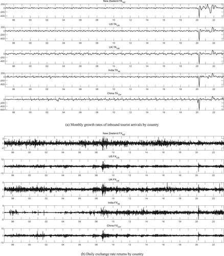
Figure 1(a) and (b) present the time path of monthly growth rates of inbound tourist arrivals by country ($\mathrm{TA}$) and daily exchange rate returns ($\mathrm{FX}$) by country, respectively. Consider, for example, Australia’s inbound tourists from New Zealand. It is observed that $T{A}_{\mathrm{NZ},t}$ exhibited significant variability after the COVID-19 pandemic in March 2020, while $F{X}_{\mathrm{NZ},t}$ demonstrated more variations during the 2008 financial crisis. However, there is no obvious evidence supporting a clear relationship between $T{A}_{\mathrm{NZ},t}$ and $F{X}_{\mathrm{NZ},t}$, thereby requiring further analysis.

Figure 1. Growth rates of inbound tourist arrivals and daily exchange rate returns. (a) Monthly growth rates of inbound tourist arrivals by country. (b) Daily exchange rate returns by country

Table 2(a) and (b) report the descriptive statistics of $\mathrm{TA}$ and $\mathrm{FX}$. As demonstrated in Table 2(a), $T{A}_{\mathrm{IN},t}$ has the highest mean growth rate (0.8847) with the standard deviation of 42.2550, reflecting a rapid increase in Australia’s inbound tourists from India. Meanwhile, the Ljung-Box test provides clear evidence supporting serial autocorrelation in $\mathrm{TA}$, while it does not demonstrate volatility clustering due to the insignificant ARCH tests. Regarding $\mathrm{FX}$ in Table 2(b), it can be seen that $F{X}_{\mathrm{IN},t}$ has the highest mean (0.7840) with the standard deviation of 0.5240, indicating that the Australian dollar showed the highest appreciation against the Indian Rupee on average over the sample period. The Ljung-Box test is significant only for the US, India, and China, reflecting serial autocorrelation in these countries’ daily exchange rate returns. The significant ARCH tests imply that daily exchange rates exhibit clear volatility clustering for all countries, supporting the use of a GARCH(1,1) model to measure daily exchange rate volatility.

Table 2. Descriptive statistics.

(a) Monthly growth rates of inbound tourist arrivals
	NZ	US	UK	IN	CH
Mean	0.2105	0.2451	0.1093	0.8847	0.5244
Std. Dev.	44.6178	40.3595	48.0998	42.2550	51.2215
Min	−486.9196	−525.0818	−563.8863	−552.7940	−632.5792
Min. Date	202004	202004	202004	202004	202004
Max	206.9685	200.6169	199.3626	201.2750	186.2140
Max. Date	202104	202111	202111	202111	202111
Ljung-Box	23.0345**	56.0414***	102.5277***	50.1424***	42.8896***
ARCH	17.4101	0.6318	0.6499	0.1604	3.4059
(b) Daily exchange rate returns
	NZ	US	UK	IN	CH
Mean (${10}^2$)	−0.0791	−0.2653	0.2177	0.7840	−0.5482
Std. Dev.	0.4508	0.7713	0.6815	0.5240	0.7584
Min	−3.1754	−7.7366	−6.6950	−6.5825	−7.8176
Min. Date	20081007	20081007	20081007	20200319	20081007
Max	3.0934	7.1562	5.9306	4.9543	7.3085
Max. Date	20081030	20081030	20160627	20200320	20081030
Ljung-Box	11.6712	34.5148***	10.2263	38.1566***	41.1560***
ARCH	1240.7004***	3262.6449***	1097.9727***	1551.4716***	2684.9353***

Notes: Ljung-Box and ARCH are the Ljung-Box tests for serial autocorrelation and GARCH effect with 12 lags. *, ** and *** indicate that the null hypothesis of test is rejected at the 10%, 5% and 1% level, respectively.

4. Empirical results and implications

4.1. Estimation results of the daily variables in the ARDL-MIDAS model

Table 3 reports the estimation results of the ARDL-MIDAS model in Equation (2)(2) $\begin{array}{rl}T{A}_{i,t+1}=& c_i+{\beta }_{\mathrm{FX}}B\left(L^{{\displaystyle \frac{1}{K}}}{\theta }_1,{\theta }_2\right)F{X}_{i,t+1}+{\beta }_{\mathrm{FXSD}}B\left(L^{{\displaystyle \frac{1}{K}}}{\gamma }_1,{\gamma }_2\right)\mathrm{FXS}{D}_{i,t+1}\\ & +\sum _{p=1}^P{\rho }_{p}T{A}_{i,t+1-p}+\sum _{q=1}^Q{\alpha }_q{X}_{q,t}+{\epsilon }_{i,t+1}.\end{array}$(2) , including estimations of the daily variables (i.e. $\mathrm{FX}$ and $\mathrm{FXSD}$) by country in Panel (a) and monthly variables (i.e. lagged $\mathrm{TA}$ and control variables) by country in Panel (b). As seen in Panel (a), the estimated ${\beta }_{\mathrm{FX}}$ is significantly negative for all the five countries, implying that daily exchange rate returns negatively affect Australia’s monthly growth rate of inbound tourist arrivals from these countries. That is, the appreciation of the Australian dollar against a foreign country’s currency will decrease Australia’s inbound tourists from that country. A-cross country comparison shows that the above negative impacts are much greater for India (−11.3107), the US (−9.8115), and China (−8.6131) due to their greater elasticities than New Zealand (−3.4847) and the UK (−2.5683). 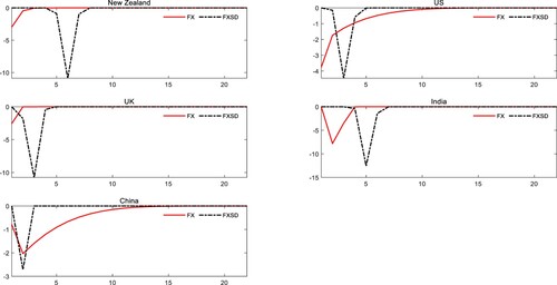As for the impact of daily exchange rate volatility, ${\beta }_{\mathrm{FXSD}}$ is significant for India (−14.3621), New Zealand (−12.7101), and the US (−5.1870). That is, apart from daily exchange rate returns, daily exchange rate volatility can also depress Australia’s inbound tourism sector. Moreover, from the magnitude of the estimated coefficients, it can be argued that inbound tourists from New Zealand and India are more sensitive to daily exchange rate volatility than daily exchange rate returns.

Table 3. Estimation results of the ARDL-MIDAS model.

(a) Daily FX and FXSD
	NZ	US	UK	IN	CH
$c_i$	4.0494 (3.8021)	5.1196 (5.0926)	−4.1363 (5.7056)	5.1226 (5.0429)	6.1165 (5.0007)
${\beta }_{\mathrm{FX}}$	−3.4847*** (1.1177)	−9.8115*** (1.8151)	−2.5683*** (0.6909)	−11.3107*** (1.6446)	−8.6131** (2.4924)
${\theta }_1$	1.0078*** (0.1135)	0.9850*** (0.0181)	0.8485*** (0.0566)	21.9641*** (0.5050)	1.0365*** (0.0607)
${\theta }_2$	44.4791 (99.5281)	6.6517*** (1.5007)	17.2220*** (2.9740)	299.9695*** (25.4874)	6.2602** (2.8304)
${\beta }_{\mathrm{FXSD}}$	−12.7101*** (2.4484)	−5.1870** (2.0186)	−12.9625 (8.4615)	−14.3621*** (2.5011)	−2.7122 (1.9990)
${\gamma }_1$	93.5375*** (4.2076)	18.3856*** (0.8496)	17.1218*** (0.0232)	72.3978*** (4.6542)	2.4031 (2.6972)
${\gamma }_2$	299.9818*** (10.0914)	171.5173*** (25.7394)	165.3652*** (22.1731)	299.9946*** (14.4291)	241.8481*** (23.8180)
(b) Monthly autoregressive terms and control variables
	NZ	US	UK	IN	CH
${\rho }_1$	−0.9110*** (0.1919)	−0.8344*** (0.1445)	−0.8054*** (0.1633)	−0.7842*** (0.0960)	−0.9162*** (0.0801)
${\rho }_2$	−0.0824* (0.0498)	−0.0441** (0.0220)	−0.0328 (0.0380)	−0.0709* (0.0389)	−0.0419 (0.0270)
${\rho }_3$	−0.0147 (0.0426)	0.0331 (0.0268)	0.0571*** (0.0156)	0.0352* (0.0186)	0.0145 (0.0219)
${\alpha }_{\mathrm{CPI}}$	−0.2828 (1.0930)	−1.1800 (0.9043)	−0.7559 (0.9789)	−0.1409 (0.2837)	0.5226 (0.5229)
${\alpha }_{\mathrm{GDP}}$	−0.1375 (0.6345)	1.1570 (0.7222)	−0.5164 (0.6252)	−1.5762*** (0.5963)	0.6176 (0.4239)
${\alpha }_{\mathrm{WUI}}$	−0.0084* (0.0047)	−0.0001 (0.0050)	−0.0003 (0.0039)	−0.0063 (0.0063)	0.0089 (0.0081)
${\alpha }_{\mathrm{TAV}}$	1.6511*** (0.1735)	1.3404*** (0.1966)	1.1557*** (0.2673)	1.2227*** (0.3053)	1.1889*** (0.1830)
${\alpha }_{\mathrm{TA}{V}^{-}}$	−2.9690*** (0.4133)	−2.7552*** (0.3539)	−2.5409*** (0.3412)	−2.4666*** (0.3285)	−2.6814*** (0.2258)
${\alpha }_{\mathrm{DEC}}$	14.2425*** (2.6589)	9.9416*** (2.0240)	20.5583*** (4.0282)	3.4964 (3.1650)	6.9963* (3.7555)
${\alpha }_{\mathrm{JAN}}$	4.0723 (9.6622)	11.4563 (8.6768)	−2.6058 (14.4300)	6.5881 (6.9882)	9.5643*** (2.9788)
${\alpha }_{\mathrm{COVID}}$	−97.9270*** (29.1623)	−37.6110* (21.8830)	−43.8083** (22.2562)	−18.7025** (8.7608)	−26.1992** (13.1413)
${\overline{R}}^2$	87.3727	80.8543	75.1053	75.1539	82.0521

Notes: Standard errors are presented in the brackets. *, ** and *** indicate that the null hypothesis of tests are rejected at the 10%, 5% and 1% level, respectively. ${\overline{R}}^2$ is the adjusted R-square in percentage.

Significant ${\theta }_1$, ${\theta }_2$, ${\gamma }_1$ and ${\gamma }_2$ for all countries except ${\theta }_2$ for New Zealand and ${\gamma }_1$ for China imply that the negative impacts of the daily $\mathrm{FX}$ and the daily $\mathrm{FXSD}$ on Australia’s monthly $\mathrm{TA}$ will last for some periods. Figure 2 depicts how intra-month information on $\mathrm{FX}$ and $\mathrm{FXSD}$ in the past 22 days affects $\mathrm{TA}$ in the current month by substituting $({\theta }_1,{\theta }_2)$ and $({\gamma }_1,{\gamma }_2)$ into the Beta weight function and multiplied by ${\beta }_{\mathrm{FX}}$ and ${\beta }_{\mathrm{FXSD}}$, respectively. It is observed that the impact of the daily $\mathrm{FX}$ occurs in the recent 1 day and lasts around 10 days for the US and China, which is longer than for New Zealand, the UK and India. As for the significant impact of the daily $\mathrm{FXSD}$, it takes effect in the recent 4–7 days for India and New Zealand and has no effect in the recent 1–3 days for the two countries. For the US, the above impact occurs in the recent 2–5 days, demonstrating no effect in the recent 1 day. As a result, it can be argued that $\mathrm{FX}$ has an earlier impact on $\mathrm{TA}$ than $\mathrm{FXSD}$. In other words, both daily exchange rate return and daily exchange rate volatility affect the monthly growth rate of inbound tourist arrivals but through different mechanisms.

Figure 2. Length of the impacts of exchange rates on inbound tourist arrivals.

Notes: The horizontal axis is the number of days ($K=22$) for which the impact lasts and the vertical axis is the impacts of each lagged day on the current inbound tourist arrivals.

4.2. Estimation results of the monthly variables in the ARDL-MIDAS model

The Ljung-Box test in Table 2(a) indicates that serial autocorrelation is detected in the monthly growth rate of inbound tourist arrivals ($\mathrm{TA}$), which suggests the inclusion of lagged $\mathrm{TA}$ into empirical modelling of inbound tourism demand forecasting. According to the BIC, the optimal lag $p=3$ is selected and the estimated autoregressive coefficients ${\rho }_p$ are reported in Panel (b) of Table 3. It can be seen that ${\rho }_1$ is significantly negative for all countries, ${\rho }_2$ is significantly negative for New Zealand (−0.0824), the US (−0.0441), and India (−0.0709), and ${\rho }_3$ is significantly positive for the UK (0.0571) and India (0.0352), demonstrating its mean-reverting characteristic and how the lagged information on $\mathrm{TA}$ contributes to forecast the growth rate of inbound tourist arrivals in the current month.

As for the macroeconomic differences control variables, all ${\alpha }_{\mathrm{CPI}}$, ${\alpha }_{\mathrm{GDP}}$ and ${\alpha }_{\mathrm{WUI}}$ are insignificant expect ${\alpha }_{\mathrm{GDP}}$ for India and ${\alpha }_{\mathrm{WUI}}$ for New Zealand. This finding implies that the differences of inflation rates, GDP growth rates, and WUI between Australia and its top inbound tourism sourcing countries make little contribution to inbound tourism demand forecasting.

Conversely, historical inbound tourism demand fluctuations ($\mathrm{TAV}$) significantly increase the explanatory power of the ARDL-MIDAS model and exhibit clear asymmetry ($\mathrm{TA}{V}^{-}$) due to significantly positive ${\alpha }_{\mathrm{TAV}}$ and significantly negative ${\alpha }_{\mathrm{TA}{V}^{-}}$ for all countries. It is interesting to discover that $|{\alpha }_{\mathrm{TAV}}|<|{\alpha }_{\mathrm{TAV}}+{\alpha }_{\mathrm{TA}{V}^{-}}|$ holds true for all countries except New Zealand, which indicates that $\mathrm{TAV}$ presents a greater impact during the $\mathrm{TA}$ decline phase than during the $\mathrm{TA}$ rise phase. These findings confirm that apart from the lagged inbound tourism demand, its fluctuations can provide additional information to improve the forecasting of future inbound tourism demand and present clear asymmetry. Meanwhile, the introduction of $\mathrm{TAV}$ and $\mathrm{TA}{V}^{-}$ can capture to a certain extent ups and downs shown in Australia’s inbound tourist arrivals during the COVID-19 pandemic, thereby solving the problem of the lack of seasonally adjusted data on inbound tourist arrivals after the pandemic.

In addition, significantly positive ${\alpha }_{\mathrm{DEC}}$ for all countries except India and significantly positive ${\alpha }_{\mathrm{JAN}}$ for China confirm the presence of holiday effect in either December or January. These two dummy variables also help alleviate the seasonal adjustment of inbound tourist arrivals data. Significantly negative ${\alpha }_{\mathrm{COVID}}$ for all countries show that Australia’s inbound tourist arrivals from its main souring countries experienced a substantial decline unexpectedly at the beginning of the pandemic, and New Zealand (−97.9270) had the highest decline, followed by the UK (−43.8083), the US (−37.6110), China (−26.1992) and India (−18.7025)

4.3. Results of the out-of-sample predictive performance

The benchmark model in Equation (3)(3) $T{A}_{i,t+1}=c_i+{\beta }_{\mathrm{FXM}}\mathrm{FX}{M}_{i,t}+{\beta }_{\mathrm{FXMSD}}\mathrm{FXMS}{D}_{i,t}+\sum _{p=1}^P{\rho }_{p}T{A}_{i,t+1-p}+\sum _{q=1}^Q{\alpha }_q{X}_{q,t}+{\epsilon }_{i,t+1}.$(3) and the four candidate models (i.e. AR: TAV, AR: TAV + TAV⁻, MIDAS: FX, and MIDAS: FX + FXSD) discussed in Section 3.3 are estimated and compared based on their out-of-sample predictive performance. Table 4 presents the comparison results of the $R_{\mathrm{OS}}^2$ in Equation (4)(4) $R_{\mathrm{OS}}^2=1-{\displaystyle \frac{{\sum }_{t=1}^{T_{\mathrm{OS}}}{(T{\hat{A}}_{i,t}^m-T{A}_{i,t})}^2}{{\sum }_{t=1}^{T_{\mathrm{OS}}}{(T{\hat{A}}_{i,t}^0-T{A}_{i,t})}^2}}$(4) and the $\mathrm{RMSE}$ in Equation (5)(5) $\mathrm{RMSE}={\displaystyle \frac{\sqrt{{\sum }_{t=1}^{T_{\mathrm{OS}}}{(T{\hat{A}}_{i,t}^m-T{A}_{i,t})}^2}}{\sqrt{{\sum }_{t=1}^{T_{\mathrm{OS}}}{(T{\hat{A}}_{i,t}^0-T{A}_{i,t})}^2}}}$(5) . Taking New Zealand as an example, the relative mean squared error ($\mathrm{RMSE}$) and the out-of-sample R-square ($R_{\mathrm{OS}}^2$) results of the AR: TAV model in Table 4 indicate that the$\mathrm{RMSE}$ of the AR: TAV model is 100.8155% of the benchmark model and it achieves a negative $R_{\mathrm{OS}}^2$. This finding implies that the historical monthly inbound tourism demand fluctuations in the past quarter worsen the performance of the AR: TAV model in forecasting Australia’s monthly inbound tourist arrivals from New Zealand. Likewise, the remaining three models’ $\mathrm{RMSE}$ are 94.9789% (AR: TAV + TAV^-), 85.9071% (MIDAS: FX), and 84.5081% (MIDAS: FX + FXSD) of the benchmark model, and they achieve the $R_{\mathrm{OS}}^2$ of 9.7901%, 26.1997%, and 28.5838%, respectively. That is, the decreased $\mathrm{RMSE}$ and the increased $R_{\mathrm{OS}}^2$ indicate that the inclusion of the historical monthly inbound tourism demand fluctuations as well as their asymmetry, daily exchange rate returns, and daily exchange rate volatility can provide additional intra-month information to forecast Australia’s monthly inbound tourist arrivals from New Zealand.

Table 4. Out-of-sample predictive performance.

		NZ	US	UK	IN	CH
AR: TAV	RMSE	100.8155	97.1279	99.3170	97.9043	94.8755
	$R_{\mathrm{OS}}^2$	−1.6376	5.6617	1.3614	4.1475	9.9865
	DM	0.5455	0.3222	0.4553	0.3675	0.1584
	MCS	1.0000	0.4281	0.7316	0.4551	0.3718
AR: TAV + TAV−	RMSE	94.9789	91.8622	91.1485	89.9533	87.4249
	$R_{\mathrm{OS}}^2$	9.7901	15.6133	16.9195	19.0840	23.5688
	DM	0.2232	0.1100	0.1132	0.0687*	0.0319**
	MCS	0.0736*	0.0251**	0.0526*	0.0146**	0.0111**
MIDAS: FX	RMSE	85.9071	80.3122	80.0169	81.8795	81.1868
	$R_{\mathrm{OS}}^2$	26.1997	35.4994	35.9729	32.9575	34.0870
	DM	0.0099***	0.0429**	0.0544*	0.0583*	0.0368**
	MCS	0.0000***	0.0359**	0.0422**	0.0354**	0.0377**
MIDAS: FX + FXSD	RMSE	84.5081	77.0649	80.9446	77.4970	79.3296
	$R_{\mathrm{OS}}^2$	28.5838	40.6100	34.4797	39.9421	37.0681
	DM	0.0059***	0.0293**	0.0635*	0.0438**	0.0280**
	MCS	0.0000***	0.0300**	0.0841*	0.0356**	0.0348**

Notes: The numbers of RMSE and $R_{\mathrm{OS}}^2$ are measured in percentage. *, ** and *** indicate that the null hypothesis is rejected at the 10%, 5% and 1% levels, respectively. DM is the p-value of the Diebold and Mariano (1995) test with the null hypothesis of a non-positive $R_{\mathrm{OS}}^2$ for the candidate model against the benchmark model. MCS is the p-value of the model confidence set test with the null hypothesis of equal predictive power between the candidate model and the benchmark model.

A comparison of these model’s $\mathrm{RMSE}$ and $R_{\mathrm{OS}}^2$ demonstrates that the MIDAS: FX model and the MIDAS: FX + FXSD model greatly outperform the benchmark model, the AR: TAV model, and the AR: TAV + TAV⁻ model due to their relatively higher $R_{\mathrm{OS}}^2$ and lower $\mathrm{RMSE}$, which hold true for all countries. This finding confirms that the intra-month exchange rate returns and the intra-month exchange rate volatility can provide additional information to greatly improve the out-of-sample predictions of Australia’s monthly inbound tourism demand. A close inspection of the MIDAS: FX model and the MIDAS: FX + FXSD model reveals that the intra-month exchange rate volatility information can improve the predictions of Australia’s monthly inbound tourist arrivals from all countries except the UK. A cross-country comparison of the MIDAS: FX + FXSD model shows that it achieves the best out-of-sample predictive performance for the US due to its highest $R_{\mathrm{OS}}^2$, followed by India, China, the UK, and New Zealand. In summary, regardless of country, the most important variable to improve the out-of-sample predictions of Australia’s monthly inbound tourism demand is daily exchange rate returns, followed by daily exchange rate volatility, and asymmetric historical inbound tourism demand fluctuations. Moreover, these findings are statistically supported by both the DM test and the MCS test, as shown in Table 4. The rejection of the null hypothesis with low p-values in these tests indicates that the candidate model outperforms the benchmark model in terms of predictive ability.

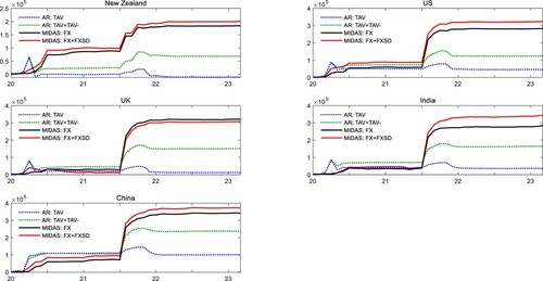
Figure 3 visualises different models’ out-of-sample predictive performance based on the$\mathrm{CSFE}$ in Equation (6)(6) $\mathrm{CSF}{E}_{i,t}^m={\sum }_{s=1}^t{(T{\hat{A}}_{i,s}^0-T{A}_{i,s})}^2-{\sum }_{s=1}^t{(T{\hat{A}}_{i,s}^m-T{A}_{i,s})}^2$(6) and provides consistent findings with Table 4. Overall speaking, the increasing $\mathrm{CSFE}$ for each candidate model reflects that these candidate models outperform the benchmark model. Moreover, the MIDAS: FX model and the MIDAS: FX + FXSD model have larger $\mathrm{CSFE}$ than the AR: TAV model and the AR: TAV + TAV⁻ model for all countries after July 2021, indicating the better out-of-sample predictive performance of the MIDAS approach. Interestingly, before July 2021, both the MIDAS: FX model and the MIDAS: FX + FXSD model did not demonstrate a significant advantage in improving the forecasting accuracy of Australia’s monthly inbound tourist arrivals from the US, the UK, India, and China. This suggests that the additional predictive power derived from the intra-month exchange rate information was quite limited during the pandemic period marked by strict travel restrictions. However, as the COVID-19 restrictions gradually eased and Australia gradually reopened its international and state borders, international travellers once again began to prioritise daily exchange rate information in planning their trips. This re-emphasizes the role of the MIDAS approach in improving the forecasting of inbound tourism demand. In other words, during the pandemic, inbound tourists’ travel decisions were heavily influenced by Australia’s travel restrictions. As economic activities gradually returned to normal with the gradual easing of the COVID-19 restrictions, their decisions were increasingly driven by the intra-month exchange rate information. This finding also holds for New Zealand around May 2020, as Australia began easing travel restrictions on inbound tourist arrivals from New Zealand earlier than other countries.

Figure 3. Out-of-sample forecasting performance.

Notes: The figure measures the relative reduction in squared forecast errors for model $m$ against the benchmark which cumulates from 2020/1 to month $t$ for country $i$. An increasing (decreasing) $\mathrm{CSFE}$ means the candidate model $m$ has smaller (larger) forecast errors and higher (lower) predictive power than the benchmark model.

4.4. Robustness check

To examine the robustness of the results derived from the MIDAS approach, this study employs the seasonal autoregressive integrated moving average and mixed data sampling (SARIMA-MIDAS) model to re-examine the relationship between inbound tourism demand and exchange rates. The SARIMA-MIDAS model demonstrates advantages in accounting for the non-linear seasonal effects of the low-frequency process and incorporating high-frequency variables into the low-frequency process using a parsimonious weighting scheme. This model proves particularly effective in capturing the observed seasonality in monthly inbound tourist arrivals with publication lags (Hu et al., 2022; Wen et al., 2021; Wu et al., 2023).

From a technical point of view, the SARIMA-MIDAS model is specified as follows: (7) $\begin{array}{rl}T{A}_{i,t+1}=& c_i+{\beta }_{\mathrm{FX}}B\left(L^{{\displaystyle \frac{1}{K}}}{\theta }_1,{\theta }_2\right)F{X}_{i,t+1}\\ & +{\beta }_{\mathrm{FXSD}}B\left(L^{{\displaystyle \frac{1}{K}}}{\gamma }_1,{\gamma }_2\right)\mathrm{FXS}{D}_{i,t+1}+\sum _{q=1}^Q{\alpha }_q{X}_{q,t}+{\eta }_{i,t+1},\end{array}$(7) (8) $\mathrm{\Phi }(B^m)\phi (B)(1-B^m{)}^D(1-B{)}^d{\eta }_{i,t+1}=\mathrm{\Theta }(B^m)\theta (B){\epsilon }_{i,t+1}.$(8) where the variables in Equation (7)(7) $\begin{array}{rl}T{A}_{i,t+1}=& c_i+{\beta }_{\mathrm{FX}}B\left(L^{{\displaystyle \frac{1}{K}}}{\theta }_1,{\theta }_2\right)F{X}_{i,t+1}\\ & +{\beta }_{\mathrm{FXSD}}B\left(L^{{\displaystyle \frac{1}{K}}}{\gamma }_1,{\gamma }_2\right)\mathrm{FXS}{D}_{i,t+1}+\sum _{q=1}^Q{\alpha }_q{X}_{q,t}+{\eta }_{i,t+1},\end{array}$(7) are defined as in Equation (2)(2) $\begin{array}{rl}T{A}_{i,t+1}=& c_i+{\beta }_{\mathrm{FX}}B\left(L^{{\displaystyle \frac{1}{K}}}{\theta }_1,{\theta }_2\right)F{X}_{i,t+1}+{\beta }_{\mathrm{FXSD}}B\left(L^{{\displaystyle \frac{1}{K}}}{\gamma }_1,{\gamma }_2\right)\mathrm{FXS}{D}_{i,t+1}\\ & +\sum _{p=1}^P{\rho }_{p}T{A}_{i,t+1-p}+\sum _{q=1}^Q{\alpha }_q{X}_{q,t}+{\epsilon }_{i,t+1}.\end{array}$(2) , except for the control variables $X_{q,t}$, which exclude the dummies representing the January and December effects. The autoregressive terms are retained in Equation (8)(8) $\mathrm{\Phi }(B^m)\phi (B)(1-B^m{)}^D(1-B{)}^d{\eta }_{i,t+1}=\mathrm{\Theta }(B^m)\theta (B){\epsilon }_{i,t+1}.$(8) . In particular, the MIDAS error term ${\eta }_{i,t+1}$ in Equation (7)(7) $\begin{array}{rl}T{A}_{i,t+1}=& c_i+{\beta }_{\mathrm{FX}}B\left(L^{{\displaystyle \frac{1}{K}}}{\theta }_1,{\theta }_2\right)F{X}_{i,t+1}\\ & +{\beta }_{\mathrm{FXSD}}B\left(L^{{\displaystyle \frac{1}{K}}}{\gamma }_1,{\gamma }_2\right)\mathrm{FXS}{D}_{i,t+1}+\sum _{q=1}^Q{\alpha }_q{X}_{q,t}+{\eta }_{i,t+1},\end{array}$(7) is further specified as a SARIMA process in Equation (8)(8) $\mathrm{\Phi }(B^m)\phi (B)(1-B^m{)}^D(1-B{)}^d{\eta }_{i,t+1}=\mathrm{\Theta }(B^m)\theta (B){\epsilon }_{i,t+1}.$(8) , where $B$ is the backshift operator. This study sets the seasonality order $m$ to 12 to account for annual seasonal effects. Both the integration order $d$ and seasonal integration order $D$ are zero as the dependent variable $T{A}_{i,t+1}$ is the monthly growth rate of inbound tourist arrivals. The non-seasonal AR component includes lags of 3 periods with coefficients of ${\rho }_1$, ${\rho }_2$, and ${\rho }_3$, while the non-seasonal MA component has a lag of 1 period with coefficient ${\vartheta }_1$. The seasonal AR components $\mathrm{\Phi }(\cdot )$ and seasonal MA component $\mathrm{\Theta }(\cdot )$ are specified as SAR(1) with the coefficients of ${\rho }_1^S$ and SMA(0), respectively, as determined by the Akaike Information Criteria (AIC).

Table 5 presents the estimation results of the SARIMA-MIDAS model. A comparison with the results from the ARDL-MIDAS model in Table 3 reveals a high degree of consistency across the majority of findings. Notably, the comparable adjusted R-squared values between the two models emphasize the importance of effectively capturing seasonality in both models to enhance forecasting accuracy for inbound tourism demand. Consequently, the robustness of the main findings derived from the ARDL-MIDAS model is affirmed.

Table 5. Estimation results of the SARIMA-MIDAS model.

(a) Daily FX and FXSD
	NZ	US	UK	IN	CH
$c_i$	5.4835 (5.9996)	4.9715 (8.9416)	−4.1385 (11.9179)	8.4619 (6.2188)	17.7288 (12.4011)
${\beta }_{\mathrm{FX}}$	−3.4270*** (1.3983)	−7.6451*** (1.7392)	−5.3118*** (0.8285)	−18.292 (4.6606)	−7.2805*** (1.9522)
${\theta }_1$	0.7686*** (0.1357)	0.9967*** (0.0267)	0.7853*** (0.0249)	1.0781*** (0.0322)	299.9003*** (48.1257)
${\theta }_2$	184.1191* (97.5422)	8.7098*** (2.7252)	17.0488*** (1.8605)	32.9270*** (8.2864)	37.4571*** (3.7083)
${\beta }_{\mathrm{FXSD}}$	−20.0526*** (3.9886)	−7.8861* (4.1629)	−12.6116 (14.7884)	−23.0495*** (4.8033)	−12.4134** (5.0201)
${\gamma }_1$	0.8392*** (0.2156)	16.5263*** (3.0813)	117.6999*** (1.2731)	112.4795*** (4.4671)	2.1328 (3.4240)
${\gamma }_2$	187.6794 (139.1732)	178.5527** (72.1791)	262.3851*** (14.3544)	299.9824*** (7.9155)	271.5260*** (65.8139)
(b) Monthly seasonal adjusted autoregressive and moving average terms and control variables
	NZ	US	UK	IN	CH
${\rho }_1$	−0.0633 (0.0513)	0.2231*** (0.0513)	−0.0558 (0.0911)	0.0567 (0.0982)	−0.6049*** (0.0149)
${\rho }_2$	−0.2161*** (0.0362)	−0.2014*** (0.0391)	−0.2218*** (0.0338)	−0.077 (0.0478)	−0.1443*** (0.0497)
${\rho }_3$	0.2909*** (0.0393)	0.2735*** (0.0384)	0.1600*** (0.0372)	0.2051*** (0.0435)	0.0064 (0.0469)
${\rho }_1^S$	−0.5665*** (0.0438)	−0.5093*** (0.0473)	−0.4020*** (0.0849)	−0.3648*** (0.0981)	0.0377 (0.0435)
${\vartheta }_1$	−0.9644*** (0.0179)	−0.9873*** (0.0144)	−0.9928*** (0.0062)	−0.9941*** (0.0072)	−0.8594*** (0.0326)
${\alpha }_{\mathrm{CPI}}$	−0.2707 (1.3858)	−1.5883 (1.0464)	−1.0023 (0.8890)	−0.4226 (0.4062)	0.2964 (0.5584)
${\alpha }_{\mathrm{GDP}}$	0.5701 (0.8044)	0.9822 (0.8542)	−0.5517 (0.7631)	−0.4085 (0.6373)	0.7799 (0.6776)
${\alpha }_{\mathrm{WUI}}$	−0.0012 (0.0075)	−0.0016 (0.0048)	−0.0023 (0.0047)	0.0041 (0.0092)	−0.0027 (0.0090)
${\alpha }_{\mathrm{TAV}}$	0.8989*** (0.0933)	0.7909*** (0.1294)	0.5520** (0.2136)	0.7382*** (0.2039)	0.4157** (0.1634)
${\alpha }_{\mathrm{TA}{V}^{-}}$	−1.1320*** (0.1794)	−1.2961*** (0.1891)	−1.2066*** (0.1947)	−1.2323*** (0.2006)	−1.1342*** (0.2154)
${\alpha }_{\mathrm{COVID}}$	−187.7761*** (49.8809)	−104.1464 (64.0122)	−91.3672 (67.4643)	−81.3768*** (27.9762)	−70.9002 (59.6717)
${\overline{R}}^2$	87.0762	81.0822	76.1490	75.3372	81.9969

Notes: Standard errors are presented in brackets. *, ** and *** indicate that the null hypotheses of tests are rejected at the 10%, 5% and 1% level, respectively. ${\overline{R}}^2$ is the adjusted R-square in percentage.

4.5. Implications

The empirical results discussed above demonstrate multiple implications for enhancing the forecasting of inbound tourism demand. First, the forecasting of monthly inbound tourism demand and daily exchange rates in Australia can be improved by using the ARDL and GARCH(1,1) models, respectively (Chang & Chang, 2020). Second, the existing knowledge regarding how exchange rates affect inbound tourism demand can be updated and deepened through the incorporation of various control variables into the proposed models. This is particularly true with the significant contributions made by historical inbound tourism demand fluctuations and their asymmetry, the holiday effect, and the COVID-19 outbreak (Shi et al., 2023). Third, the intra-month exchange rate information significantly enhances the forecasting of monthly inbound tourism demand by considering both daily exchange rate returns and daily exchange rate volatility.

The improved forecasting of inbound tourism demand further establishes the foundation for future tourism resource allocation, business planning, and policy making. For example, more accurate predictions of inbound tourist arrivals enable destinations to anticipate peak and off-peak tourist seasons more effectively. When a destination is experiencing a rise in tourism, the efficient allocation of resources to tourism is encouraged, including timely adjustments to the number of personnel and proactive planning for more facilities and infrastructure to meet the demand during the rise phase. When a decline in tourism occurs, a destination needs to make more efforts to attract a more niche market by introducing new attractions, organising new events, and upgrading existing accommodations and facilities. Tourism businesses can optimise their pricing strategies by maximising revenue during peak seasons and offering competitive prices during off-peak seasons. Government and tourism authorities in destinations can formulate effective visa policies, environmental and cultural sustainability measures based on more accurate forecasting of inbound tourist arrivals. They can emphasize capacity planning and crisis preparedness during peak tourist seasons, while giving more attention to destination repositioning and fostering public-private collaboration during off-peak seasons.

5. Conclusions

More accurate predictions of inbound tourism demand play a crucial role in assisting destinations, tourism businesses and policy makers in making better-informed decisions. Therefore, this study adopts the ARDL-MIDAS model to extract intra-month information about exchange rates, aiming to enhance the forecasting of inbound tourist arrivals to Australia. The main results are as follows: First, daily exchange rate returns negatively affect Australia’s monthly growth rate of inbound tourist arrivals from the selected source countries, supporting the statement that the appreciation of the Australian dollar against a foreign country’s currency will decrease the respective inbound tourists from that country. Meanwhile, daily exchange rate volatility can also depress Australia’s inbound tourism sector, which exhibits country disparities. Second, the monthly growth rate of inbound tourist arrivals follows a mean-reverting process and its historical fluctuation information in the past 3 months significantly increases the explanatory power of the ARDL-MIDAS model. Moreover, it is found that historical inbound tourism demand fluctuations and their asymmetry, the holiday effect, and the COVID-19 outbreak make significant contributions to the forecasting of inbound tourism demand. Third, the ARDL-MIDAS model with consideration of daily exchange rate returns and daily exchange rate volatility greatly outperforms the benchmark model and the other three candidate models, supporting that the intra-month information about exchange rates significantly improves the forecasting of monthly inbound tourism demand.

Despite the profound methodological and policy implications generated by the above empirical results, this study can still be extended in various ways. For example, as an alternative measurement of inbound tourism demand, inbound tourist expenditures by country can be used as a robustness analysis in future research when their data availability is improved. Another way to deepen the present study is to acknowledge the limitations of the ARDL-MIDAS model in terms of overfitting due to the inclusion of too many variables, interpretability due to the complexity of the model, weight function determination, and computational intensity due to the use of large datasets. These extensions pave the way for future research.

Credit author statement

Yuting Gong: Software, Methodology, Original draft preparation, Visualisation. Mengjie Jin: Writing-Reviewing and Editing. Kum Fai Yuen: Writing-Reviewing and Editing. Xueqin Wang: Writing-Reviewing and Editing. Wenming Shi: Conceptualisation, Methodology, Writing-Reviewing, Investigation and Editing.

Disclosure statement

No potential conflict of interest was reported by the author(s).

Additional information

Funding

This work was supported by National Natural Science Foundation of China through grant number 71971133 (Yuting Gong). This work was supported by the National Natural Science Foundation of China (grant nos. 72203088; Mengjie Jin) and the Ministry of Education in China, Humanities and Social Science Project [grant number 21YJC790055; Mengjie Jin].

Notes

1 https://www.unwto.org/tourism-data/global-and-regional-tourism-performance

2 https://www.tra.gov.au/ArticleDocuments/185/STSA%202018-19%20Report.pdf.aspx

3 https://www.abs.gov.au/statistics/industry/tourism-and-transport/overseas-arrivals-and-departures-australia/jun-2023#visitor-arrivals-short-term-financial-year-2022-23 (ABS 2023: Australian Bureau of Statistics).

4 https://www.tra.gov.au/en/economic-analysis/tourism-satellite-accounts/national-tourism-satellite-account#ref8 (NTAS, 2023: National Tourism Satellite Account).

5 Australia’s monthly growth rates of inbound tourist arrivals from New Zealand, the US, the UK, India, and China experienced a dramatic decline in March and April 2020 (see Figure 1), which remained relatively stable after April 2020. To capture the unexpected decline, the COVID-19 outbreak dummy variable is defined, and it takes the value of 1 in March and April 2020.

References

- Ahir, H., Bloom, N., & Furceri, D. (2022). The world uncertainty index. No. w29763. National Bureau of Economic Research. https://doi.org/10.3386/w29763
- Akay, G. H., Cifter, A., & Teke, O. (2017). Turkish tourism, exchange rates and income. Tourism Economics, 23(1), 66–77. https://doi.org/10.5367/te.2015.0497
- Alola, U. V., Cop, S., & Alola, A. A. (2019). The spillover effects of tourism receipts, political risk, real exchange rate, and trade indicators in Turkey. International Journal of Tourism Research, 21(6), 813–823. https://doi.org/10.1002/jtr.2307
- Andreou, E., Ghysels, E., & Kourtellos, A. (2013). Should macroeconomic forecasters use daily financial data and how? Journal of Business & Economic Statistics, 31(2), 240–251. https://doi.org/10.1080/07350015.2013.767199
- Barman, H., & Nath, H. K. (2019). What determines international tourist arrivals in India? Asia Pacific Journal of Tourism Research, 24(2), 180–190. https://doi.org/10.1080/10941665.2018.1556712
- Bicak, H. A., Altinay, M., & Jenkins, H. (2005). Forecasting the tourism demand of North Cyprus. Journal of Hospitality & Leisure Marketing, 12(3), 87–99. https://doi.org/10.1300/J150v12n03_06
- Canbay, Ş., Coşkun, İ. O., & Kırca, M. (2023). Symmetric and asymmetric frequency-domain causality between tourism demand and exchange rates in Türkiye: A regional comparison. International Journal of Emerging Markets. https://doi.org/10.1108/IJOEM-06-2022-0899
- Chang, K. L., & Chang, J. C. D. (2020). Dynamic dependence between US inbound visits and exchange rate. Journal of Hospitality & Tourism Research, 44(6), 1035–1046. https://doi.org/10.1177/1096348020913084
- Cheng, K. M. (2012). Tourism demand in Hong Kong: Income, prices, and visa restrictions. Current Issues in Tourism, 15(3), 167–181. https://doi.org/10.1080/13683500.2011.569011
- Chi, J. (2015). Dynamic impacts of income and the exchange rate on US tourism, 1960-2011. Tourism Economics, 21(5), 1047–1060. https://doi.org/10.5367/te.2014.0399
- Cró, S., & Martins, A. M. (2017). Structural breaks in international tourism demand: Are they caused by crises or disasters? Tourism Management, 63, 3–9. https://doi.org/10.1016/j.tourman.2017.05.009
- De Vita, G. (2014). The long-run impact of exchange rate regimes on international tourism flows. Tourism Management, 45, 226–233. https://doi.org/10.1016/j.tourman.2014.05.001
- De Vita, G., & Kyaw, K. S. (2013). Role of the exchange rate in tourism demand. Annals of Tourism Research, 43, 624–627. https://doi.org/10.1016/j.annals.2013.07.011
- Diebold, F. X., & Mariano, R. S. (1995). Comparing predictive accuracy. Journal of Business & Economic Statistics, 13(3), 253–263. https://doi.org/10.1080/07350015.1995.10524599
- Dogru, T., Isik, C., & Sirakaya-Turk, E. (2019). The balance of trade and exchange rates: Theory and contemporary evidence from tourism. Tourism Management, 74, 12–23. https://doi.org/10.1016/j.tourman.2019.01.014
- Dogru, T., Sirakaya-Turk, E., & Crouch, G. I. (2017). Remodeling international tourism demand: Old theory and new evidence. Tourism Management, 60, 47–55. https://doi.org/10.1016/j.tourman.2016.11.010
- Dritsakis, N., & Athanasiadis, S. (2000). An econometric model of tourist demand. Journal of Hospitality & Leisure Marketing, 7(2), 39–49. https://doi.org/10.1300/J150v07n02_03
- Dwyer, L., Forsyth, P., & Rao, P. (2002). Destination price competitiveness: Exchange rate changes versus domestic inflation. Journal of Travel Research, 40(3), 328–336. https://doi.org/10.1177/0047287502040003010
- Eilat, Y., & Einav, L. (2004). Determinants of international tourism: A three-dimensional panel data analysis. Applied Economics, 36(12), 1315–1327. https://doi.org/10.1080/000368404000180897
- Falk, M. (2015). The sensitivity of tourism demand to exchange rate changes: An application to Swiss overnight stays in Austrian mountain villages during the winter season. Current Issues in Tourism, 18(5), 465–476. https://doi.org/10.1080/13683500.2013.810610
- Ghartey, E. E. (2013). Effects of tourism, economic growth, real exchange rate, structural changes and hurricanes in Jamaica. Tourism Economics, 19(4), 919–942. https://doi.org/10.5367/te.2013.0228
- Ghosh, S. (2022). Modelling inbound international tourism demand in Australia: Lessons from the pandemics. International Journal of Tourism Research, 24(1), 71–81. https://doi.org/10.1002/jtr.2483
- Ghysels, E., Sinko, A., & Valkanov, R. (2007). MIDAS regressions: Further results and new directions. Econometric Reviews, 26(1), 53–90. https://doi.org/10.1080/07474930600972467
- Hailemariam, A., & Dzhumashev, R. (2023). The impact of pandemic induced uncertainty shock on tourism demand. Current Issues in Tourism, 26(16), 2575–2581. https://doi.org/10.1080/13683500.2022.2113044
- Hansen, P. R., Lunde, A., & Nason, J. M. (2011). The model confidence set. Econometrica, 79(2), 453–497. https://doi.org/10.3982/ECTA5771
- Harvey, H., & Furuoka, F. (2019). The role of tourism, real exchange rate and economic growth in Singapore: Are there asymmetric effects? Journal of Tourism and Hospitality Management, 7(2), 64–84. https://doi.org/10.15640/jthm.v7n2a8
- Hu, M., Li, H., Song, H., Li, X., & Law, R. (2022). Tourism demand forecasting using tourist-generated online review data. Tourism Management, 90, 104490. https://doi.org/10.1016/j.tourman.2022.104490
- Imamboccus, R., Seetanah, B., Jaffur, Z. K., & Nunkoo, R. (2024). The exchange rate; its volatility and tourism demand. Anatolia 1–13. https://doi.org/10.1080/13032917.2024.2303639
- Karimi, M. F., Khan, A. A., & Karamelikli, H. (2018). Asymmetric effects of real exchange rate on inbound tourist arrivals in Malaysia: An analysis of price rigidity. International Journal of Tourism Research, 21(2), 156–164. https://doi.org/10.1002/jtr.2249
- Kim, J., & Lee, C. K. (2017). Role of tourism price in attracting international tourists: The case of Japanese inbound tourism from South Korea. Journal of Destination Marketing & Management, 6(1), 76–83. https://doi.org/10.1016/j.jdmm.2016.03.002
- Kuok, R. U. K., Koo, T. T. R., & Lim, C. (2023). Economic policy uncertainty and international tourism demand: A global vector autoregressive approach. Journal of Travel Research, 62(3), 540–562. https://doi.org/10.1177/00472875211072551
- Lee, S. K., & Jang, S. C. S. (2011). Foreign exchange exposure of US tourism-related firms. Tourism Management, 32(4), 934–948. https://doi.org/10.1016/j.tourman.2010.08.008
- Lee, J. J., Lee, Y. M., & Huang, S. J. (2018). Dynamic relationships among tourist arrivals, crime rate, and macroeconomic variables in Taiwan. Asia Pacific Journal of Tourism Research, 23(9), 896–906. https://doi.org/10.1080/10941665.2018.1500380
- Lim, S. K., & Giouvris, E. (2020). Tourist arrivals in Korea: Hallyu as a pull factor. Current Issues in Tourism, 23(1), 99–130. https://doi.org/10.1080/13683500.2017.1372391
- Lim, C., & Zhu, L. (2017). Dynamic heterogeneous panel data analysis of tourism demand for Singapore. Journal of Travel & Tourism Marketing, 34(9), 1224–1234. https://doi.org/10.1080/10548408.2017.1330173
- Lin, Y. C., & Deng, W. S. (2018). Are per capita international tourist arrivals converging? International Review of Economics & Finance, 57, 274–290. https://doi.org/10.1016/j.iref.2018.01.013
- Martins, L. F., Gan, Y., & Ferreira-Lopes, A. (2017). An empirical analysis of the influence of macroeconomic determinants on World tourism demand. Tourism Management, 61, 248–260. https://doi.org/10.1016/j.tourman.2017.01.008
- Meo, M. S., Chowdhury, M. A. F., Shaikh, G. M., Ali, M., & Sheikh, S. M. (2018). Asymmetric impact of oil prices, exchange rate, and inflation on tourism demand in Pakistan: New evidence from nonlinear ARDL. Asia Pacific Journal of Tourism Research, 23(4), 408–422. https://doi.org/10.1080/10941665.2018.1445652
- Muchapondwa, E., & Pimhidzai, O. (2011). Modelling international tourism demand for Zimbabwe. International Journal of Business and Social Science, 2, 71–81.
- Ozturk, I. (2006). Exchange rate volatility and trade: A literature survey. International Journal of Applied Econometrics and Quantitative Studies, 3. SSRN: https://ssrn.com/abstract=1127299
- Santana-Gallego, M., Ledesma-Rodríguez, F. J., & Pérez-Rodríguez, J. V. (2010). Exchange rate regimes and tourism. Tourism Economics, 16(1), 25–43. https://doi.org/10.5367/000000010790872015
- Schiff, A., & Becken, S. (2011). Demand elasticity estimates for New Zealand tourism. Tourism Management, 32(3), 564–575. https://doi.org/10.1016/j.tourman.2010.05.004
- Seetanah, B., & Sannassee, R. V. (2015). Marketing promotion financing and tourism development: The case of Mauritius. Journal of Hospitality Marketing & Management, 24(2), 202–215. https://doi.org/10.1080/19368623.2014.914359
- Seetaram, N. (2010). Use of dynamic panel cointegration approach to model international arrivals to Australia. Journal of Travel Research, 49(4), 414–422. https://doi.org/10.1177/0047287509346992
- Sharma, M., Mohapatra, G., & Giri, A. K. (2023). The determinants of inbound tourism demand in India: New evidence from ARDL co-integration approach. Business Perspectives and Research, 1–14.
- Sharma, C., & Pal, D. (2020). Exchange rate volatility and tourism demand in India: Unraveling the asymmetric relationship. Journal of Travel Research, 59(7), 1282–1297. https://doi.org/10.1177/0047287519878516
- Shi, W., Gong, Y., Wang, L., & Nikolova, N. (2023). Heterogeneity of inbound tourism driven by exchange rate fluctuations: Implications for tourism business recovery and resilience in Australia. Current Issues in Tourism, 26(3), 450–467. https://doi.org/10.1080/13683500.2021.2023478
- Shi, W., & Li, K. X. (2017). Impact of unexpected events on inbound tourism demand modeling: Evidence of Middle East Respiratory Syndrome outbreak in South Korea. Asia Pacific Journal of Tourism Research, 22(3), 344–356. https://doi.org/10.1080/10941665.2016.1250795
- Song, H., Qiu, R. T. R., & Park, J. (2023). Progress in tourism demand research: Theory and empirics. Tourism Management, 94, 104655. https://doi.org/10.1016/j.tourman.2022.104655
- Song, H., & Witt, S. F. (2000). Tourism demand modelling and forecasting: Modern econometric approaches. Routledge.
- Tang, J., Sriboonchitta, S., Ramos, V., & Wong, W. K. (2016). Modelling dependence between tourism demand and exchange rate using the copula-based GARCH model. Current Issues in Tourism, 19(9), 876–894. https://doi.org/10.1080/13683500.2014.932336
- Wang, M. Y., Li, Y. Q., Ruan, W. Q., Zhang, S. N., & Li, R. (2024). Influencing factors and formation process of cultural inheritance-based innovation at heritage tourism destinations. Tourism Management, 100, 104799. https://doi.org/10.1016/j.tourman.2023.104799
- Wen, L., Liu, C., Song, H., & Liu, H. (2021). Forecasting tourism demand with an improved mixed data sampling model. Journal of Travel Research, 60(2), 336–353. https://doi.org/10.1177/0047287520906220
- Wu, J., Li, M., Zhao, E., Sun, S., & Wang, S. (2023). Can multi-source heterogeneous data improve the forecasting performance of tourist arrivals amid COVID-19? Mixed-data sampling approach. Tourism Management, 98, 104759. https://doi.org/10.1016/j.tourman.2023.104759
- Yazdi, S. K., & Khanalizadeh, B. (2017). Tourism demand: A panel data approach. Current Issues in Tourism, 20(8), 787–800. https://doi.org/10.1080/13683500.2016.1170772
- Zhu, L., Lim, C., Xie, W., & Wu, Y. (2018). Modelling tourist flow association for tourism demand forecasting. Current Issues in Tourism, 21(8), 902–916. https://doi.org/10.1080/13683500.2016.1218827