Remembrances of things past: evidence from a twenty-year Kerala panel

ABSTRACT

We construct a panel of 242 households from five consecutive Kerala Migration Surveys that span 20 years at five-year intervals to study the fundamental determinants of the decision to migrate abroad as well as the decision to remit. Accounting for time-invariant unobservables and allowing migration and remittance behavior to depend upon previous choices clarifies our understanding of both decisions. Migration and remittance behavior display positive serial correlation over a five-year time horizon and the presence of a return migrant in the household increases the likelihood of migration by 13% and remittances by 4%. Migration is 1% more likely in female-headed households, 4% less likely when the household head is employed, increases by 0.4% for each additional year of the household head's age and is 6% more likely in households that are asset-poor. Remittances are between 20% and 70% more likely to obtain when the migrant was married at the time of migration and 3% less likely when the household head is employed, the latter suggesting either an old-age security or a co-insurance motive. Evidence in favor of a very strong inheritance competition motive is found in that each additional male heir increases the likelihood of remittances by between 8% and 31%. Based on our econometric evidence, and in particular our findings pertaining to serial correlation and the presence of a return migrant in the household, it is likely that both migration from and remittances to Kerala will quickly rebound to their pre-pandemic levels.

1. Introduction

An important limitation of most of the economics literature on migration and remittances is that it is based either on cross-sectional data or on longitudinal datasets which cover a very short time-span.¹ In this paper, we present new evidence on the characteristics of migrants, as well as their behavior, using a unique panel dataset that allows us to follow a sample of 242 Keralite households over the twenty year period spanning 1998 to 2018, at five-year intervals.

There are at least two reasons why constructing such data is important. First, long panel data allow one to gauge life-cycle aspects of the migration phenomenon that are invisible using cross-sectional data or short panels: to wit, the modeling of migration and remittance behavior can explicitly incorporate lagged dependent variables.

Second, it allows one to account for time-invariant characteristics of migrants and their households that are likely to be correlated with the migration and remittance decisions, on the one hand, and various time-varying household and migrant characteristics, on the other. When such correlated time-invariant unobservables are appropriately controlled for, it turns out that many cross-sectional correlations disappear (and others appear) or, more importantly, are reversed in sign. Thus, such data can (and do) fundamentally change our understanding of the determinants of migration and remittance behavior. The length of the panel does come at a cost however, in that there is a relatively limited number of covariates that can be taken into account. For example, data on the income of the households in Kerala is missing for several of the KMS surveys that we link to form our panel, as is data on the income of migrants. The same is true of details concerning migration costs and the skills of migrants before and after their migration experience.² Nevertheless, the tradeoff is, in our opinion, a favorable one, and falls squarely within the remit of the new economics of labor migration, as set out in Stark and Bloom (1985). The estimates we obtain also allow one to formulate a number of predictions concerning the impact of the COVID-19 pandemic on Kerala return migration, and place it within its South and South-East Asian context (Rajan and Arcand 2023), based on this quantitative historical evidence.

Finally, Kerala's inclusion in this special issue is warranted because of its status both as a prominent sending region representing a significant share of Indian emigrants overseas, as well as being a microcosm of South and Southeast Asian migration patterns, categorized by unemployment of the educated, the preponderance of remittances in the share of GDP, and the downstream cultural influence of migration in the socioeconomic evolution of the region (Skeldon 2006).

2. The evolution of migration over twenty years

We begin by establishing a series of stylized facts concerning migration in Kerala by linking five KMS surveys collected at five-year intervals between 1998 and 2018.

2.1. Univariate statistics

Kerala is a state strongly characterized by migration, and many households receive remittances. This is illustrated in the four panels of Figure 1. Figure 1(a) below shows that at any point in time, approximately 1 in 3 households either have a current migrant or have a member of the household who has returned from migration. More than 15% of households have at least one member who was in migration at the time of any one of the five surveys. Figure 1(b) shows that Muslim households are more likely to have a migrant than Hindu or Christian households. It is also apparent, in the same figure, that most of the migration is international, and overwhelmingly to the Gulf countries, especially for Muslim households. The peak of migration was in 2008, when 1 in 3 households had at least one current migrant abroad or elsewhere in India; Muslim households display the same amount of within-India migration as Christians and Hindus. The figures also suggest that migration flows returned to their pre-2008 levels.

Figure 1. Share of households with migrants and receiving remittances, by type of migrant and by religion, 1998–2018. (a) Share of households with migrants, by type of migrant. (b) Share of households with migrants, by religion, 1998–2018. (c) Share of households receiving remittances, by type of migrant. (d) Share of households receiving remittances, by religion, 1998–2018.

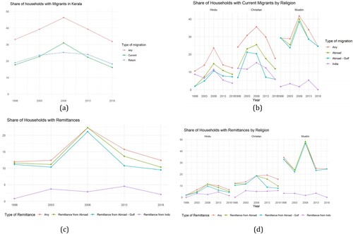
Figure 1(c) shows that not all households which have migrants abroad receive remittances back from them. There is heterogeneity by type of household and by type of migration. The peak of remittance receipts, 2008, coincides with the year of peak migration; almost 1 in 4 households received some remittances. We can see from Figure 1(d) that Muslim households, which are the ones typically having a migrant in the Gulf, are also more likely to receive remittances than Hindu or Christian households.

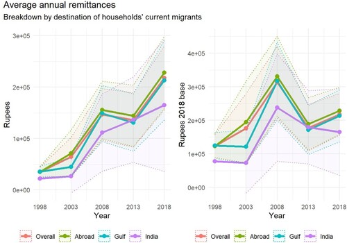
Figure 2 shows that the average monetary value of remittances increased over time (left-hand panel), but that their real value did less so (right-hand panel). The peak was in 2008, it dropped in 2013 and increased again in 2018. The amount of remittances is relatively large when compared with household earnings. We compute the share of average monthly remittances with respect to average household earnings for 2013 and 2018 as these are the only two KMS waves with information on household earnings. Average monthly remittances represented 97% and 130% of household earnings for 2013 and 2018, respectively.

Figure 2. Average annual remittances, by origin, current and constant monetary values, 1998–2018.

2.2. A profile of migrants

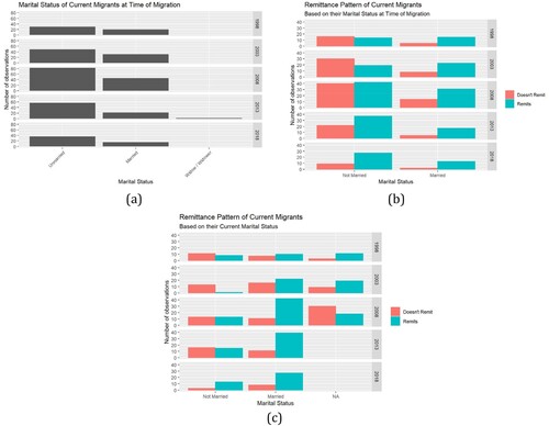
As shown in Figure 3(a) migrants are typically the married sons of the household head. Most of these are the eldest sons, as shown in Figure 3(b). They are older and more likely to be married. In each wave, and as shown in Figure 4(a), they were more likely to be unmarried than married at the time of migration. Concomitantly, migrants who were married at the time of migration are much more likely to remit than the unmarried ones, as shown in Figure 4(b). Currently married migrants are also more likely to remit than the unmarried ones, as shown in Figure 4(c).

Figure 3. Household position (by gender) and birth-order by marital status of current migrants, 1998–2018. (a) Household position of migrants, by gender, averages for the 1998–2018 period. (b) Birth-order and marital status of current migrants, 1998–2018.

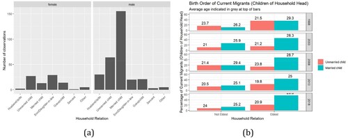
Figure 4. Marital status and remittance patterns of migrants, at the time of migration and based on their current marital status, 1998–2018. (a) Marital status of current migrants at the time of migration, 1998–2018. (b) Remittance patterns by marital status of current migrants at the time of migration, 1998–2018. (c) Remittance behavior and current marital status of the migrant, 1998–2018.

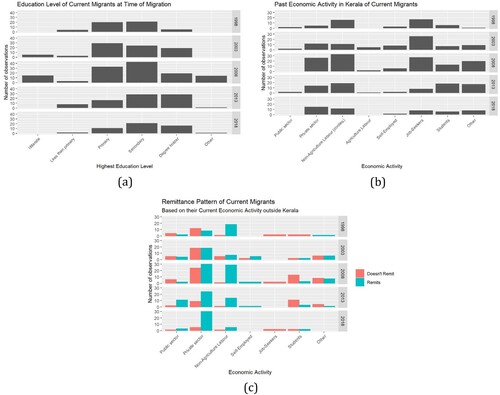
The migrants' highest level of education at time of migration was mostly either primary or secondary level schooling: this is shown in Figure 5(a). At the time of migration, and as shown in Figure 5(b), a migrant's most common economic activity was to be either a job-seeker, to be employed in the private sector or to be be a laborers in non-agriculture sector. There were very few who were employed either in the public sector or as agriculture laborers. Once they migrate, the migrants mostly work in the private sector, as shown in Figure 5(c); they are also typically the ones sending remittances back home to Kerala.

Figure 5. Educational attainment, past economic activity and remittances, 1998–2018. (a) Educational attainment of migrants at the time of migration, 1998–2018. (b) Past economic activity in Kerala of current migrants, 1998–2018. (c) Remittance behavior and current economic activity outside Kerala of migrants, 1998–2018.

2.3. The life cycle of migrant households

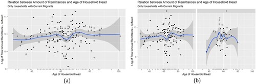
We have seen that many migrant and household characteristics are correlated with both the migration and the remittance decision. Perhaps the most interesting bivariate relationship concerning a household's migration life-cycle involves the relationship between the age of the household head and the magnitude of the remittances received. In Figure 6 we display a non-parametric smooth of the relationship between the age of the household head and the logarithm of the total remittances received by the household. The most striking aspect of Figure 6(a) is that there are two peaks in the receipt of remittances over the household's life-cycle: one when the household head is between 55 and 60 years old, and the other when he reaches 70–75. The average age of household heads at the birth of their first child is approximately 28, while the average age at migration is also 28. Thus, one way to understand this ‘twin peaks’ phenomenon is that the first bump coincides with an eldest child (typically a son) migrating and reimbursing the migration costs incurred by the household. In contrast, the second bump corresponds to what are essentially old age insurance payments. The plausibility of this interpretation is strengthened in Figure 6(b) which divides the sample into unemployed (0) and employed (1) household heads. While the twin peaks appear in these figures, the first bump is more prominent than the second for employed household heads, which is to be expected in that retirement support is less needed when the household head has a job (or perhaps receives a pension from previous employment). Female household heads, who are relatively rare, display a peak for remittances somewhat later in their life-cycle: this corresponds once again to old age insurance.³

Figure 6. Twin peaks in remittance behavior with respect to the age of the household head, and with respect to the latter's employment status, 1998–2018. Blue lines are non-parametric smooths; gray shaded area corresponds to the 95% confidence interval. (a) Log total remittances and the age of the household head, 1998–2018. (b) Log total remittances and the age of the household head: household head not employed on the left, employed on the right, 1998–2018.

3. Econometric evidence

3.1. Specifications

The descriptive statistics and bivariate relationships presented so far have allowed us to paint a picture of the typical migrant as evidenced by our unique panel dataset. In order to delve into these issues more deeply, and to untangle the key characteristics driving both migration and remittance behavior, we must take a multivariate approach which allows us to study all of these factors while controlling for the others.

A first empirical specification is given by: (1) $y_{it}=x_{it}\text{β}+{\lambda }_i+{\mu }_t+{ϵ}_{it},$(1) where i indexes households and t KMS survey years, while $y_{it}$ is either a dummy variable indicating that the household has a member who is a migrant or a dummy indicating that the household receives remittances.⁴ The matrix $x_{it}$ of covariates is given by a series of household and migrant characteristics. Finally, unobservables are decomposed into time-invariant (${\lambda }_i$) and KMS year-specific (${\mu }_t$) effects, with ${ϵ}_{it}$ representing time-varying household specific unobservables. The main advantage of the panel data we are using is that it allows us to sweep out time-invariant unobservables ${\lambda }_i$ through a within-household transformation, thereby dealing with the potential correlation between these unobservables and the covariates that would bias the estimates of the parameter vector β. For example, if time-invariant unobservable factors have a positive effect on the likelihood of international migration and are simultaneously associated with a higher number of adult males in the household, then the coefficient associated with the latter will be biased upwards in a regression where the dependent variable is whether the household has an international migrant or not. Indeed, suppose for argument's sake that there is actually no effect of the number of adult males on migration. In that case, we might incorrectly conclude that the correlation exists by dint of the fact that we failed to adequately control for time-invariant unobservables. The opposite conclusion (i.e. downward bias) would hold if the correlation between the time-invariant unobservables and the number of adult males were negative, leading us to fail to detect what might be a true increasing relationship.

Whether these configurations are indeed the case, and whether or not being able to control for correlated household-specific unobservables fundamentally changes our understanding of the migration and remittance questions, is one focus of what follows. Note that the effect of all time-invariant covariates (such as the household's religion) cannot be identified when one controls for household fixed effects: this limitation is, however, more than compensated for by the elimination of any spurious correlation due to unobserved time-invariant heterogeneity.

A second advantage of the twenty year length of our panel is that it allows us to explicitly incorporate dynamics into our econometric specification. While matched pairs of KMS datasets have previously allowed one to control for household-specific unobservables that remain constant between adjoining KMS waves, it has not been possible to follow the same households over a significant portion of the household's life cycle using, to be explicit, lagged dependent and explanatory variables. Here we are able to do so using a dynamic panel specification (which accounts for the biases introduced by lagged dependent variables in fixed effects regressions), introduced into the econometrics literature by Arellano and Bond (1991), Anderson and Hsiao (1981) and Arellano and Bover (1995). A potentially richer alternative to the specification given in (1(1) $y_{it}=x_{it}\text{β}+{\lambda }_i+{\mu }_t+{ϵ}_{it},$(1) ) is therefore provided by: (2) $y_{it}=y_{it-1}\alpha +x_{it}\text{β}+x_{it-1}\gamma +{\lambda }_i+{\mu }_t+{ϵ}_{it},$(2) where we can therefore allow for lag(s) of the dependent variable, as well as of the covariates. Identification in first differences (which sweeps out the household-specific time-invariant unobservables) is achieved through the usual moment restrictions based on lagged levels of the observables, while identification in levels is achieved through lags of the first-differenced variables. This is, of course, our preferred specification in that the moment conditions, when they are valid, account for correlated time-varying unobservables, thereby taking care of both endogeneity and measurement error. Note that there is nothing ‘magical’ about such GMM procedures: in essence they simply correspond to a statistically efficient instrumental variables procedure, where the instruments are the variables themselves in lagged and lagged first-differenced form. As with any instrumental variables procedure, they will only properly deal with endogeneity and measurement error issues (which often, though not always, lead to attenuation bias) when the underlying maintained hypotheses are satisfied. In this regard, the key maintained assumption of no second-order serial correlation is tested through the standard $m_2$ test of Arellano and Bond (1991). Standard errors are calculated using the double-correction method recently introduced by Hwang, Kang, and Lee (2022). Note that Equations (1(1) $y_{it}=x_{it}\text{β}+{\lambda }_i+{\mu }_t+{ϵ}_{it},$(1) ) and (2(2) $y_{it}=y_{it-1}\alpha +x_{it}\text{β}+x_{it-1}\gamma +{\lambda }_i+{\mu }_t+{ϵ}_{it},$(2) ) are both linear probability models and that the coefficients can therefore be interpreted as linear approximations to the underlying marginal effects of the covariates on the probability of having a migrant or of remitting.

Table 1 presents descriptive statistics for the variables used in our econometric specifications. As should be obvious from the last two columns of the table, it is most often the case that the within-household standard deviation of a variable represents at least two-thirds of its total standard deviation: as such, the estimators that we adopt, and which account for time-invariant heterogeneity through fixed effects or first-differencing, make sense from a statistical standpoint because there is much within-household variation for identification purposes.⁵ Concomitantly, our covariance transformations in the fixed effects and GMM specifications mop up between-household residual variance, which is far from being negligible.

Table 1. Descriptive statistics corresponding to Tables 2 and 3.

	Mean	St. Dev.	within-hh St. Dev.
Household has an international migrant	0.230	0.421	0.290
Household has an international migrant, t−5	0.235	0.424	0.293
Household receives remittances	0.157	0.364	0.266
Household receives remittances, t−5	0.156	0.363	0.263
Female household head	0.226	0.419	0.271
Household head is employed	0.494	0.500	0.359
Age of household head	60.295	13.009	8.506
Migrant was married at time of migration	0.098	0.298	0.237
Number of male heirs	0.290	0.774	0.545
Asset-poor household	0.405	0.491	0.358
Log number adult males in household	1.300	0.448	0.290
Return migrant in household	0.227	0.419	0.283
Return migrant in household, t−5	0.229	0.421	0.304

Table 2. Dependent variable: household has an international migrant.

	OLS	FE	OLS	FE	GMM	FE	GMM
	(1)	(2)	(3)	(4)	(5)	(6)	(7)
Household has an international migrant, t−5			${0.419}^{\ast \ast \ast }$	$-0.051$	$-{0.003}^{\ast }$	$-0.046$	${0.015}^{\ast \ast \ast }$
			$\left(0.048\right)$	$\left(0.054\right)$	$\left(0.002\right)$	$\left(0.056\right)$	$\left(0.004\right)$
Female household head	${0.166}^{\ast \ast \ast }$	${0.169}^{\ast \ast \ast }$	${0.109}^{\ast \ast \ast }$	${0.181}^{\ast \ast \ast }$	${0.001}^{\ast }$	${0.181}^{\ast \ast \ast }$	${0.009}^{\ast \ast \ast }$
	$\left(0.050\right)$	$\left(0.051\right)$	$\left(0.032\right)$	$\left(0.056\right)$	$\left(0.000\right)$	$\left(0.055\right)$	$\left(0.003\right)$
Household head is employed	$-{0.090}^{\ast \ast }$	$-0.017$	$-{0.068}^{\ast \ast \ast }$	$-0.016$	$-0.001$	$-0.016$	$-{0.041}^{\ast \ast \ast }$
	$\left(0.036\right)$	$\left(0.040\right)$	$\left(0.024\right)$	$\left(0.047\right)$	$\left(0.001\right)$	$\left(0.047\right)$	$\left(0.010\right)$
Age of household head	$-0.008$	$-0.001$	$-0.003$	$-0.003$	${0.006}^{\ast \ast \ast }$	$-0.003$	${0.004}^{\ast \ast \ast }$
	$\left(0.008\right)$	$\left(0.006\right)$	$\left(0.006\right)$	$\left(0.008\right)$	$\left(0.001\right)$	$\left(0.008\right)$	$\left(0.001\right)$
Age of household head, squared	0.000	$-0.000$	0.000	$-0.000$	$-{0.000}^{\ast }$	$-0.000$	$-0.000$
	$\left(0.000\right)$	$\left(0.000\right)$	$\left(0.000\right)$	$\left(0.000\right)$	$\left(0.000\right)$	$\left(0.000\right)$	$\left(0.000\right)$
Log number adult males in household	${0.270}^{\ast \ast \ast }$	${0.286}^{\ast \ast \ast }$	${0.238}^{\ast \ast \ast }$	${0.352}^{\ast \ast \ast }$	${0.000}^{\ast \ast \ast }$	${0.351}^{\ast \ast \ast }$	${0.022}^{\ast \ast \ast }$
	$\left(0.044\right)$	$\left(0.047\right)$	$\left(0.039\right)$	$\left(0.059\right)$	$\left(0.000\right)$	$\left(0.059\right)$	$\left(0.005\right)$
Asset-poor household	${0.106}^{\ast \ast \ast }$	0.041	${0.085}^{\ast \ast \ast }$	0.036	${0.001}^{\ast \ast }$	0.035	${0.057}^{\ast \ast \ast }$
	$\left(0.028\right)$	$\left(0.029\right)$	$\left(0.027\right)$	$\left(0.036\right)$	$\left(0.000\right)$	$\left(0.036\right)$	$\left(0.013\right)$
Return migrant in household	0.004	$-{0.177}^{\ast \ast \ast }$	$-{0.074}^{\ast \ast }$	$-{0.150}^{\ast \ast \ast }$	$-{0.003}^{\ast }$	$-{0.149}^{\ast \ast \ast }$	${0.078}^{\ast \ast \ast }$
	$\left(0.041\right)$	$\left(0.039\right)$	$\left(0.035\right)$	$\left(0.054\right)$	$\left(0.001\right)$	$\left(0.054\right)$	$\left(0.017\right)$
Return migrant in household, t−5						0.021	${0.055}^{\ast \ast \ast }$
						$\left(0.040\right)$	$\left(0.013\right)$
Adjusted $R^2$	0.127	0.449	0.291	0.458	$0.458$
Hansen J: $p-$value					0.967		0.730
AR2: $p-$value					0.705		0.681

${}^{\ast \ast \ast }p<0.01$; ${}^{\ast \ast }p<0.05$; ${}^{\ast }p<0.1$ Notes: Columns (1) and (3): OLS. Columns (2), (4) and (6): household-specific fixed effects. Standard errors, clustered at the taluk level in columns (1)–(4) and (6), in parentheses. Columns (5) and (7): Arellano and Bover (1995) first-differences and levels GMM estimation, with Hwang, Kang, and Lee (2022) double-corrected standard errors in parentheses. 242 households each observed five times at five year intervals, 1998–2008.

Table 3. Dependent variable: household receives remittances.

	OLS	FE	GMM	GMM	GMM
	(1)	(2)	(3)	(4)	(5)
Household receives remittances, t−5	${0.123}^{\ast \ast \ast }$	$-0.040$	${0.063}^{\ast }$	${0.131}^{\ast \ast \ast }$	${0.077}^{\ast }$
	$\left(0.038\right)$	$\left(0.071\right)$	$\left(0.033\right)$	$\left(0.047\right)$	$\left(0.042\right)$
Household has an international migrant	${0.441}^{\ast \ast \ast }$		${0.467}^{\ast \ast \ast }$
	$\left(0.067\right)$		$\left(0.067\right)$
Migrant was married at time of migration	0.118	${0.328}^{\ast \ast \ast }$	${0.203}^{\ast \ast \ast }$	${0.401}^{\ast \ast \ast }$	${0.704}^{\ast \ast \ast }$
	$\left(0.078\right)$	$\left(0.093\right)$	$\left(0.074\right)$	$\left(0.092\right)$	$\left(0.115\right)$
Number of male heirs	${0.082}^{\ast \ast \ast }$	${0.179}^{\ast \ast \ast }$	${0.082}^{\ast \ast \ast }$	${0.198}^{\ast \ast \ast }$	${0.311}^{\ast \ast \ast }$
	$\left(0.024\right)$	$\left(0.039\right)$	$\left(0.022\right)$	$\left(0.030\right)$	$\left(0.043\right)$
Number of male heirs * married at time of migration					$-{0.272}^{\ast \ast \ast }$
					$\left(0.057\right)$
Asset-poor household	$-{0.036}^{\ast \ast }$	$-0.008$	$-{0.024}^{\ast }$	$-0.011$	$-0.022$
	$\left(0.016\right)$	$\left(0.020\right)$	$\left(0.013\right)$	$\left(0.015\right)$	$\left(0.014\right)$
Household head is employed	$-{0.040}^{\ast \ast }$	$-{0.064}^{\ast \ast \ast }$	$-{0.030}^{\ast \ast \ast }$	$-{0.037}^{\ast \ast \ast }$	$-{0.029}^{\ast \ast }$
	$\left(0.018\right)$	$\left(0.025\right)$	$\left(0.011\right)$	$\left(0.013\right)$	$\left(0.013\right)$
Age of household head	$-0.001$	$-0.001$	$-{0.000}^{\ast \ast }$	$-0.000$	$-0.000$
	$\left(0.001\right)$	$\left(0.001\right)$	$\left(0.000\right)$	$\left(0.000\right)$	$\left(0.000\right)$
Return migrant in household	${0.039}^{\ast \ast \ast }$	0.022	${0.040}^{\ast }$	${0.043}^{\ast }$	${0.039}^{\ast }$
	$\left(0.014\right)$	$\left(0.044\right)$	$\left(0.021\right)$	$\left(0.022\right)$	$\left(0.021\right)$
Adjusted $R^2$	0.590	0.519
Hansen J: $p-$value			0.001	0.002	0.002
AR2: $p-$value			0.660	0.739	0.425

${}^{\ast \ast \ast }p<0.01$; ${}^{\ast \ast }p<0.05$; ${}^{\ast }p<0.1$ Notes: Columns (1) and (3): OLS. Columns (2), (4) and (6): household-specific fixed effects. Standard errors, clustered at the taluk level in columns (1)–(4) and (6), in parentheses. Columns (5) and (7): Arellano and Bover (1995) first-differences and levels GMM estimation, with Hwang, Kang, and Lee (2022) double-corrected standard errors in parentheses. 242 households each observed five times at five year intervals, 1998–2008.

3.2. Existing econometric evidence

Previous econometric studies on international migration from, and international remittances to, Kerala that are related to the present paper are relatively rare, though they are all related in some manner to the KMS surveys. Koola and Ozden (2008) use data from the 1998 and 2003 KMS surveys to examine the impact of geographic and religious networks on the migration decision, the choice of destination, as well as the effect of migration on the likelihood of unemployment and job seeking. They also consider the impact of being unemployed, a job seeker or an international migrant household in 1998 on the same variables in 2003. However, given that they only use two years of data, they are unable to control for time-invariant unobservables and their specifications boil down to cross sectional regressions.⁶

Antoniades et al. (2018) use a field experiment to construct a proxy for altruism (from the willingness to share in a standard dictator game) for a sample of 105 male married blue-collar migrant workers from Kerala working in Qatar. They find that annual remittances are unrelated to the migrant's degree of altruism, and that the marginal propensity to remit out of (migrant) income, the only statistically significant covariate, is 0.60. No other migrant or (home) household characteristics appear to matter. The exception is the subsample of 46 migrants with a loan obligation (76% of which are property-related), for whom altruism significantly increases annual remittances. They explain this finding with a theoretical model of reference-dependent preferences in the tradition of Koszegi and Rabin (2006) in which a loan obligation brings more certainty about the reference point for remittances.

Pattath (2020), using the 2011 and 2016 linked KMS surveys, finds that individual relative deprivation and group relative deprivation, measured using the standard (Yitzhaki 1979) index, both increase the likelihood of international migration when the reference group is based on religion, while controlling for time-invariant unobservables. The theoretical argument underlying the use of relative deprivation as the key explanatory variable is that of conspicuous consumption on the part of migrants returning from the Gulf.

Finally, Seshan (2020) compares the asset gains (using standard (Filmer and Pritchett 2001) first principal component asset indices) to households in Kerala who have a member who moves overseas to those with someone who migrates within India. He uses a first-difference specification over the 1998 and 2003 KMS surveys that accounts for time-invariant household unobservables. Despite international migrants displaying lower levels of skill than their domestic counterparts, the international wage premium they enjoy appears to compensate, leading to no statistically significant difference in assets gains between the two categories of Keralite migrant households.⁷

3.3. Findings: migration

Table 2 reports results from estimating Equations (1(1) $y_{it}=x_{it}\text{β}+{\lambda }_i+{\mu }_t+{ϵ}_{it},$(1) ) and (2(2) $y_{it}=y_{it-1}\alpha +x_{it}\text{β}+x_{it-1}\gamma +{\lambda }_i+{\mu }_t+{ϵ}_{it},$(2) ), where the dependent variable is a dummy which is equal to 1 when the household has an international migrant abroad and zero otherwise. There are significant differences in the statistical significance, signs and magnitudes of the estimated coefficients reported in Table 2 as we move from OLS (where we therefore do not account for ${\lambda }_i$), to household fixed effects, to system GMM estimation, thereby progressively better addressing a number of statistical issues. Note that, for the GMM results reported in columns (5) and (7) the overidentifying restrictions are not rejected by the usual Hansen $J-$statistic and the null of the absence of second-order serial correlation is not rejected by the Arellano-Bond $m_2$ test, with the richer specification of column (7) which allows for both contemporaneous and lagged effects of there being a return migrant in the household, being our preferred model.

Four covariates have an unambiguous effect (in terms of its sign) on the likelihood of the household having at least one international migrant, irrespective of the underlying econometric specification, though the magnitudes and statistical significance of the effects often differ appreciably. First, the household head being female unambiguously increases the likelihood of having an international migrant. The household head being a woman is often associated with widowhood, and is robust to controlling for time-invariant unobservables: we can identify the effect of this variable because there are many households for which the gender of the household head changes over the twenty year period of observation (otherwise, the within-household standard deviation of this variable would have been equal to zero, which it manifestly is not), which usually corresponds to a male household head dying and being replaced in that role by his spouse. In the preferred GMM specification of column (7) the marginal effect corresponds to a 1% increase in the likelihood of having an international migrant, which is significantly lower (in absolute value) than the 10 to 18% effects that obtain (see columns (1) –(4) and (6)) when time-varying unobservables are not taken into account.

Second, the household head being employed is associated with a 4% drop in the likelihood of there being an international migrant in column (7), while the effect is either significantly larger (in absolute value) or statistically indistinguishable from zero in all other cases. Note that the GMM results of column (7) account for endogeneity so this effect is not being driven by reverse causality in which household heads are less likely to be employed because the household has a member working abroad. That this is the case is suggested by the OLS results of columns (1) and (3) being significantly larger (in absolute value) since they presumably fail to account for time-varying unobservables that are driving both migration and the likelihood of the household head being unemployed. This variable is often associated with an ‘intertemporal contract’ form of migration, in which the household funds the migration of an adult male abroad, expecting him later to contribute to household finances through remittances later on. Migration, in this case, is an investment decision undertaken by the household.

Third, the (log) number of prime-age males in the household significantly increases the likelihood of there being a migrant. In column (7) the size of this effect is one order of magnitude smaller than in specifications that do not take time-varying unobservables into account, though it is still statistically significant at conventional levels of confidence. It should be obvious that an additional adult male facilitates the household's continuing productive activities at home, while simultaneously benefitting from the remittances stemming from the young man sent abroad as a migrant.

Fourth, the household being asset-poor is associated with a significant increase in the likelihood of there being a migrant. The household asset index should be seen as a proxy for wealth. As in Seshan (2020), the index is calculated based on the paper by Filmer and Pritchett (2001) by using principal components analysis (PCA). This technique extracts the orthogonal linear combination of the included variables that best explains the shared information. In our case, the characteristics included are household assets which appear in every wave of the survey: whether the household owns a tv, a fridge, a motorcycle, a taxi, the cooking fuel used, and the type of house (from kutcha (mud house) to luxurious). The first principal component is the index for household wealth. Following again Filmer and Pritchett (2001), households in the bottom 40% are considered as poor, the next 40% as middle-class and the top 20% as rich.

The impact of two other covariates – the lagged dependent variable and the presence of a return migrant in the household – are particularly sensitive to the econometric specification, and highlight the advantages of constructing long panel data that allows one to take the intra-household dynamics of the migration phenomenon seriously. In columns (3) the OLS results suggest a very high degree of first-order correlation (over a five year horizon) in the household's possessing an international migrant, while this effect becomes negative (though statistically insignificant) once household-specific unobservables are controlled for in column (4). Moving to GMM estimation in column (5) tightens the precision of this negative point estimate, while the fixed effects estimates of column (6), which allow for a (5 year) lagged effect of the presence of a return migrant in the household, lead to the point estimate of the lagged dependent variable becoming statistically insignificant.

In this specification (column (6)), it is also the case that the contemporaneous effect of the presence of a return migrant significantly reduces the likelihood of migration. Finally, once time-varying unobservables are taken into account in the GMM estimates of column (7), we see that first-order serial correlation in the dependent variable is small, positive and precisely estimated, while the presence of a return migrant – in contemporaneous and lagged form – significantly increase the likelihood of migration. This last effect is essentially the phenomenon that ‘migration begets migration’ with dynamics of household members going, returning to the household and going again being the key. It also highlights that intra-household experience in terms of migration is a central driving force of migration in Kerala, which complements the migration network phenomena at the community level that have been highlighted in other contexts by Munshi (2014) and Munshi and Rosenzweig (2016).

3.4. Findings: remitting

Since the seminal paper of Lucas and Stark (1985), it has been commonplace to distinguish between altruistic and co-insurance versus investment and implicit contract justifications for remittances.⁸ For the former, the migrant's motivation to remit is based on altruistic preferences which imply, for example, that remittances should be (inversely) correlated with shocks to the migrant's (recipient household's) income stream. A similar argument sees remittance behavior when household heads are elderly as a form of old-age insurance. For the latter, the motivation to remit is entirely based on an implicit intertemporal contract between migrant and home household head.

Results are presented in Table 3. The econometric specifications are slightly less successful than in the case of the migration decision per se in that the tests of the overidentifying restrictions reject. On the other hand, the null of the absence of second-order serial correlation is never rejected in the three GMM specifications presented in columns (3) to (5).

Four results stand out. First, remittances are between 20% and 70% more likely to obtain when the migrant was married at the time of migration: the only specification in which the migrant's marital status does not affect remittances is that presented in column (1) where the effect of marital status is in all likelihood being picked up by the dummy which indicates whether the household has a migrant abroad amongst its members. This is suggested both by the fact that the equivalent specification in column (2), which drops the migrant dummy, yields a marginal impact of the marital status of the migrant of 32.8% which is estimated quite precisely. Notice also that the inclusion of the migrant dummy always leads to a decrease of roughly 20 percentage points in the marginal impact of the migrant's marital status on the probability of remitting: from 32.8% in column (2) to 11.8% in column (1), and from 40.1% in column (4) to 20.3% in column (3). This is suggestive of an implicit contract explanation (Poirine 1997) mediated through the presence of the migrant's spouse in the home household. Essentially, the migrant's spouse plays the role of a ‘hostage’ the existence of whom induces the migrant to repay the migration costs initially incurred by the family in sending him abroad.

Second, when the household head is employed, the GMM estimates of columns (3) to (5) yield a fall in the probability of remitting of approximately 3%. The corresponds either to an old-age security or a co-insurance motive, or both. This is reminiscent of the findings for small island nations of Brown, Connell, and Jimenez-soto (2014): remittances play what is essentially a social security role. Altruistic preferences of the migrant towards his family will reinforce this effect, since an altruistic motive predicts higher (lower) remittances when the family's income is relative low (high). It is also consonant with the investment hypothesis alluded to earlier: the family invests in sending the migrant abroad, and remittances then represent a ‘return’ on that initial investment when the household head back home is no longer able to work. This is, of course, particularly salient in contexts, such as Kerala, where limited opportunities for funding retirement are available.

Third, evidence for a strong inheritance competition motive is found in the very precisely estimated coefficient associated with the number of male heirs. This variable is constructed as the number of brothers for current migrants who are sons of the household head, thereby capturing the patrilineal blood line, and there are very few cases in which two sons are both migrants. Each additional male heir increases the probability of a migrant remitting by between 8% and 31%. This would also be consistent with a fall in the bargaining power of the migrant in the spirit of Cox (1987). In this case, remittances are seen as a payoff to the family in which the winner will gain a larger share of any available inheritance. Notice also that the household being asset-poor has a relatively weak negative impact on remittances: while the point estimate is always negative, it is often statistically indistinguishable from zero at usual levels of confidence (in columns (2), (4) and (5)). Thus, while competition among male siblings for the inheritance may be important, the magnitude of the inheritance per se, as measured by assets, does not play a quantitatively important role in determining remittance behavior. Note also, in the results presented in column (5) that the interaction of the number of male heirs and being married at the time of migration yields a negative coefficient: a priori, this indicates that already being married at the time of migration increases the bargaining power of the migrant relative to any male siblings, thereby leading to lower levels of remittances.

Finally, and perhaps most importantly from the COVID-19 perspective, note that there is significant positive serial correlation in remittance behavior, with the household's having received remittances five years earlier being associated, ceteris paribus, with an almost 8% higher likelihood of it receiving remittances today.

4. The impact of COVID-19

The estimates presented in this paper allow one to sketch, based on 20 years of historical data, the likely impact of the COVID-19 pandemic on return migration and remittances in Kerala. The key explanatory variables from this perspective are, of course, the lagged dependent variables and the presence of a return migrant in the household. Recent estimates suggest that almost two thirds of Keralites living abroad returned home during the May 2020–April 2021 period, due to the COVID pandemic, amounting to 1.4 million individuals. Based on our preferred estimates from the first line of column (7) of Table 2, we would expect, five year later, that the number of migrants would be reduced by roughly 1.4m × 0.015 = 21,000 individuals through this dynamic effect– already a relatively small number. This number, moreover, would be tempered –and perhaps be more than overcompensated for, by the impact of having a very large number of return migrants living at home, as implied by the positive coefficients reported in the last two lines of column (7). As such, it is likely that the total number of migrants will return to, and perhaps exceed, its pre-COVID-19 level relatively quickly. In terms of remittances, the prediction of our econometric estimates is similar: the positive serial correlation in remittance behavior will result in a temporary fall in remittances with respect to their pre-COVID level. But again, the presence of a large number of return migrants in the household should result in remittances returning relatively quickly to their pre-pandemic levels.

Are these predictions concerning COVID-19 reasonable when compared to the response of migration and remittances to other large-scale shocks in the past? If we consider the pre- and post-2008 pattern of migration in our sample, as is displayed in Figure 1(a), it is worth noting that there was a significant increase in the proportion of households with international migrants during the boom years of 2003–2008. Following the international financial crisis of 2008, the share of households with migrants essentially returned to its 1998 level. Similarly, and as shown in right-hand panel of Figure 2 (which plots the value of remittances in real terms over time in our sample) remittances steadily increased during the boom of 2003–2008 and then suffered a large fall after 2008, but follow a roughly similar pre-financial crisis growth path after 2013. As such, our econometric results, and their implications for the effect of COVID-19, are in line with the relative long-run stability of migration and remittance flows in the past.

Of course, our long-run data do not allow us to account for short-term phenomena such as wage theft, considered in the Sri Lankan context by Weeraratne (2023), or other negative experiences suffered by Kerala migrants such as those studied in Rajan, Pattath, and Tohidimehr (2023), in Nepal (Adhikari et al. 2023), or in Pakistan (Farooq and Arif 2023). Such experiences can have long-run scarring effects in terms of migrant behavior. Similarly, and on a more positive note, we are not able to provide quantitative evidence on the impact on migration of post-COVID reintegration policies in the country of origin, such as those considered by Opiniano and Ang (2023) in the Filipino context. That being said, our econometric results suggest, based on the quantitative historical evidence, that Kerala migration and remittances will rapidly rebound to their pre-pandemic levels, and continue to provide an important source of livelihoods for the households that remain at home.

Disclosure statement

No potential conflict of interest was reported by the author(s).

Notes

1 See the standard surveys by Rapoport and Docquier (2006) or Brown and Jimenez-Soto (2015).

2 The role of migrant skills, and how they combine with informational asymmetries to induce return migration, is considered by Stark (1995).

3 Not presented but available upon request.

4 In what follows, we confine our attention to a linear probability model and eschew non-linear specifications. The marginal effects obtained using the corresponding conditional logit specifications are very similar to the linear probability model results and are omitted in the interests of brevity. Note that households for which the second dummy variable is equal to one is necessarily a subset of the households for which the first dummy variable is equal to one.

5 If within-household standard deviations were a mere fraction of their total standard deviation counterparts, then these covariance transformations would risk exacerbating measurement error problems by leading to one essentially regressing noise on noise. See Griliches and Hausman (1986) for the standard reference.

6 Standard errors should also have been clustered at the panchayet level, since the key network variables are constructed at that level of aggregation. Given the likely positive intra-class correlation within panchayets, it is probable that the reported standard errors are significantly underestimated.

7 The IV procedures are somewhat curious in that two of the proposed excluded instruments (the household being Muslim and the number of male household members aged between 19 and 40 in the 1998 survey round) are time-invariant and instrument the number of migrants who left the household between survey rounds. It is difficult to see the impact of these IVs affecting the change in assets between survey rounds solely through their effect on the number of individuals leaving the household, as is required for them to be admissible. Moreover, the third proposed IV (the change in the number of male members between 1998 and 2003) is better seen as a first-differenced covariate that should be included in the first-differenced structural equation from the start.

8 Agarwal and Horowitz (2002) distinguish between altruism and risk-sharing and come down, using data from Guyana, squarely in favor of the former.

References

- Adhikari, Jagannath, Mahendra Kumar Rai, Mahendra Subedi, and Chiranjivi Baral. 2023. “Foreign Labour Migration in Nepal in Relation to COVID-19: Analysis of Migrants’ Aspirations, Policy Response and Policy Gaps from Disaster Justice Perspective.” Journal of Ethnic and Migration Studies 49 (20): 5219–5237. https://doi.org/10.1080/1369183X.2024.2268983.
- Agarwal, Reena, and Andrew W Horowitz. 2002. “Are International Remittances Altruism or Insurance? Evidence from Guyana Using Multiple-migrant Households.” World Development 30 (11): 2033–2044. https://doi.org/10.1016/S0305-750X(02)00118-3.
- Anderson, T. W., and C. Hsiao. 1981. “Estimation of Dynamic Models with Error Components.” Journal of the American Statistical Association 76 (375): 598–606. https://doi.org/10.1080/01621459.1981.10477691.
- Antoniades, Alexis, Ganesh Seshan, Roberto Weber, and Robertas Zubrickas. 2018. “Does Altruism Matter for Remittances?” Oxford Economic Papers 70 (1): 225–242. https://doi.org/10.1093/oep/gpx035.
- Arellano, M., and S. Bond. 1991. “Some Tests of Specification of Panel Data: Monte Carlo Evidence and an Application to Employment Equations.” The Review of Economic Studies 58 (2): 277–297. https://doi.org/10.2307/2297968.
- Arellano, Manuel, and Olympia Bover. 1995. “Another Look at the Instrumental Variable Estimation of Error-Components Models.” Journal of Econometrics 68 (1): 29–51. https://doi.org/10.1016/0304-4076(94)01642-D.
- Brown, Richard P., John Connell, and Eliana V. Jimenez-soto. 2014. “Migrants' Remittances, Poverty and Social Protection in the South Pacific: Fiji and Tonga.” Population, Space and Place 20 (5): 434–454. https://doi.org/10.1002/psp.v20.5.
- Brown, Richard P., and Eliana V. Jimenez-Soto. 2015. “Migration and Remittances.” In Barry R. Chiswick and Paul W. Miller (eds.), Handbook of the Economics of International Migration (Vol.1, pp. 1077–1140). North-Holland Elsevier.
- Cox, Donald. 1987. “Motives for Private Income Transfers.” Journal of Political Economy 95 (3): 508–546. https://doi.org/10.1086/261470.
- Farooq, Shujaat, and G. M. Arif. 2023. “The Facts of Return Migration in the Wake of Covid-19: A Policy Framework for Reintegration of Pakistani Workers.” Journal of Ethnic and Migration Studies 49 (20): 5190–5218. https://doi.org/10.1080/1369183X.2024.2268976.
- Filmer, Deon, and Lant H. Pritchett. 2001. “Estimating Wealth Effects Without Expenditure Data- or Tears: An Application to Educational Enrollments in States of India.” Demography 38 (1): 115.
- Griliches, Zvi, and Jerry A Hausman. 1986. “Errors in Variables in Panel Data.” Journal of Econometrics31 (1): 93–118. https://doi.org/10.1016/0304-4076(86)90058-8.
- Hwang, Jungbin, Byunghoon Kang, and Seojeong Lee. 2022. “A Doubly Corrected Robust Variance Estimator for Linear GMM.” Journal of Econometrics 229 (2): 276–298. https://doi.org/10.1016/j.jeconom.2020.09.010.
- Koola, Jinu, and Caglar Ozden. 2008. “Should I Stay or Should I Go: Geographic Versus Cultural Networks in Migration and Employment Decisions.” In World Bank, Annual Bank Conference on Development Economics, Cape Town, South Africa.
- Koszegi, B., and M. Rabin. 2006. “A Model of Reference-Dependent Preferences.” The Quarterly Journal of Economics 121 (4): 1133–1165. https://doi.org/10.1093/qje/121.1.121.
- Lucas, Robert E. B., and Oded Stark. 1985. “Motivations to Remit: Evidence from Botswana.” Journal of Political Economy 93 (5): 901–918. https://doi.org/10.1086/261341.
- Munshi, Kaivan. 2014. “Community Networks and the Process of Development.” Journal of Economic Perspectives 28 (4): 49–76. https://doi.org/10.1257/jep.28.4.49.
- Munshi, K., and Mark R. Rosenzweig. 2016. “Networks and Misallocation: Insurance, Migration, and the Rural-Urban Wage Gap.” American Economic Review 106 (1): 46–98. https://doi.org/10.1257/aer.20131365.
- Opiniano, Jeremiah, and Alvin Ang. 2023. “Should I Stay Or Should I Go? Analysing Returnee Overseas Filipino Workers’ Reintegration Measures Given The COVID-19 Pandemic.” Journal of Ethnic and Migration Studies 49 (20): 5281–5304. https://doi.org/10.1080/1369183X.2024.2268992.
- Pattath, Balasubramanyam. 2020. “Keeping up with Kerala's Joneses.” In India Migration Report 2020, edited by S. Irudaya Rajan, 23–54. London: Routledge India.
- Poirine, Bernard. 1997. “A Theory of Remittances as an Implicit Family Loan Arrangement.” World Development 25 (4): 589–611. https://doi.org/10.1016/S0305-750X(97)00121-6.
- Rajan, S. Irudaya, and Jean Louis Arcand. 2023. “Covid-19 Return Migration Phenomena: Experiences from South and Southeast Asia.” Journal of Ethnic and Migration Studies 49 (20): 5133–5152. https://doi.org/10.1080/1369183X.2024.2268963.
- Rajan, S. Irudaya, Balasubramanyam Pattath, and Hossein Tohidimehr. 2023. “The Last Straw? Experiences and Future Plans of Returned Migrants in the India-GCC Corridor.” Journal of Ethnic and Migration Studies 49 (20): 5169–5189. https://doi.org/10.1080/1369183X.2024.2268970.
- Rapoport, Hillel, and F. Docquier. 2006. "The Economics of Migrants' Remittances." In Handbook of the Economics of Giving, Altruism and Reciprocity, S.-C. Kolm, and J. Mercier Ythier, 1135–1198. North-Holland Publ Co.
- Seshan, Ganesh K. 2020. “Migration and Asset Accumulation in South India: Comparing Gains to Internal and International Migration from Kerala.” World Bank Policy Research Working Paper, 9237.
- Skeldon, Ronald. 2006. “Interlinkages Between Internal and International Migration and Development in the Asian Region.” Population, Space and Place 12 (1): 15–30. https://doi.org/10.1002/(ISSN)1544-8452.
- Stark, Oded. 1995. “Return and Dynamics: The Path of Labor Migration When Workers Differ in Their Skills and Information is Asymmetric.” The Scandinavian Journal of Economics 97 (1): 55. https://doi.org/10.2307/3440829.
- Stark, Oded, and David E. Bloom. 1985. “The New Economics of Labor Migration.” American Economic Review 75 (2): 173–178.
- Weeraratne, B. 2023. “COVID-19 Pandemic Induced Wage Theft: Evidence from Sri Lankan Migrant Workers.” Journal of Ethnic and Migration Studies 49 (20): 5259–5280. https://doi.org/10.1080/1369183X.2024.2268989.
- Yitzhaki, Shlomo. 1979. “Relative Deprivation and the Gini Coefficient.” Quarterly Journal of Economics93 (2): 321–324. https://doi.org/10.2307/1883197.