Comparison of statistical analysis methods for object case best–worst scaling

Abstract

Aims: Different methods have been used to analyze “object case” best–worst scaling (BWS). This study aims to compare the most common statistical analysis methods for object case BWS (i.e. the count analysis, multinomial logit, mixed logit, latent class analysis, and hierarchical Bayes estimation) and to analyze their potential advantages and limitations based on an applied example.

Methods: Data were analyzed using the five analysis methods. Ranking results were compared among the methods, and methods that take respondent heterogeneity into account were presented specifically. A BWS object case survey with 22 factors was used as a case study, tested among 136 policy-makers and HTA experts from the Netherlands, Germany, France, and the UK to assess the most important barriers to HTA usage.

Results: Overall, the five statistical methods yielded similar rankings, particularly in the extreme ends. Latent class analysis identified five clusters and the mixed logit model revealed significant preference heterogeneity for all, with the exception of three factors.

Limitations: The variety of software used to analyze BWS data may affect the results. Moreover, this study focuses solely on the comparison of different analysis methods for the BWS object case.

Conclusions: The most common statistical methods provide similar rankings of the factors. Therefore, for main preference elicitation, count analysis may be considered as a valid and simple first-choice approach. However, the latent class and mixed logit models reveal additional information: identifying latent segments and/or recognizing respondent heterogeneity.

Keywords:

• Analysis
• best–worst scaling
• comparison
• methods
• object case

Introduction

Due to the need for a more patient-centered approach in healthcare and more acknowledgment of health technology assessment (HTA) in decision-making, it is increasingly important to elicit the preferences of patients and of healthcare providers in the process of support for making health policy and clinical decisions^1,2. Preference studies may help to identify potential differences between stakeholders (enhancing patient-centered healthcare)³ and can provide relevant information to support HTA and the setting of evidence-based priorities in healthcare⁴. Conjoint analyses are useful for eliciting preferences and rankings. This is a decomposition method that derives implicit values for factors from an overall score for a profile consisting of two or more factors⁵. One type of conjoint analysis is becoming increasingly popular in healthcare research, i.e. the best–worst scaling (BWS)^6,7. BWS has advantages compared to other conjoint analyses methods, such as discrete choice experiments (DCEs), as BWS elicits not only information on the most preferred but also on the least preferred option⁸. There are three types of BWS: in “object case” BWS (also called case 1) a list of factors are ranked based on best–worst choice tasks, while the factors in “profile” case BWS (also called case 2) are levels of attributes (in which each choice task represents a profile), and in “multi-profile” case BWS (also called case 3) there are complete profiles (consisting of several characteristics; similar to a DCE). In particular, “object case” BWS is useful for incorporating a relatively large number of factors (compared to other types of BWS experiments and DCEs) and may be less cognitively burdensome (which is especially important when eliciting preferences from vulnerable groups^6,9). A typical object case BWS experiment consists of choice tasks with a minimum of three unique factors, in which the participant is asked to indicate the best and the worst factor. The overall aim is to obtain a full ranking of factors, which can then be analyzed in several ways⁷.

In recent systematic reviews of BWS, the most important and popular statistical methods for analyzing the object case BWS were identified, i.e. the count analysis, multinomial logit, mixed logit (or random parameter model), latent class analysis, and hierarchical Bayes estimation^6,7. Methods used ranged from simple count analysis to more advanced statistical models taking respondent heterogeneity into account. Count analysis is limited to examining choice frequencies and may be applied at the group level as well as the individual level¹⁰. When BWS is used to investigate the likelihood that a factor is identified as most important or least important, one needs dual coding, best (yes or no) and worst (yes or no). Multinomial logit and mixed logit yield propensity scores, reflecting the likelihood of a factor being present in a given combination. In recent years, we observed increased interest and use of models that incorporate respondent heterogeneity in the analyses, such as the latent class model and the mixed-logit model⁶. These models allow assessing how the results differ among respondents. The mixed logit model provides information on the distribution of parameters, incorporating respondent heterogeneity. The latent class, a form of cluster analysis, allows the identification of latent groups, which is useful when there is hidden respondent heterogeneity caused by differences in choice behavior that may not be linked to observable socio-economic characteristics¹¹.

To the best of our knowledge, no study has yet comprehensively compared different common statistical methods for analyzing object case BWS. In comparing various BWS analysis methods, an earlier applied study¹² found results to be similar for the paired model conditional logit analysis and the marginal model conditional logit analysis. Also, agreement between summary analyses using weighted least squares and estimates from multinomial models was found to be high. Although previous literature showed that hierarchical Bayes and count analyses were applied most often in BWS studies in healthcare, other methods were also used⁶. Indeed, different methods are used in the scientific literature to analyze best–worst data, and BWS-specific guidelines are still developing¹³. In light of this, it is important to assess whether the various most commonly used statistical methods yield similar results or not, and to assess the potential added value and limitations of each analysis technique for future research in this field.

This paper reports on an empirical comparison between different analytical methods, using data from a BWS study that quantifies the importance of barriers to the usage of HTA in several European countries. This study, therefore, aims (i) to explore the comparability of the five most common analysis methods for object case BWS: (1) count analysis, (2) multinomial logit, (3) mixed logit, (4) latent class analysis, and (5) hierarchical Bayes estimation, and (ii) to analyze their potential advantages and limitations.

Methods

The BWS survey

For the purpose of this study, we used a previous object case BWS that aimed to quantify the relative importance of barriers and facilitators regarding the use of HTA in policy decisions^14,15. Our study focuses on the object case BWS only for barriers to the use of HTA. The relevant list of factors was developed based on a scoping review and expert validation¹⁴. This led to a final list of 22 barriers (see Table 1). Questionnaires were generated using Sawtooth¹⁶, yielding fractional, efficient designs. The final survey was designed and distributed online using Qualtrics¹⁷. Data were collected in the Netherlands, Germany, France, and the UK. Each participant was asked to choose the most important and least important barrier to the uptake of HTA in 14 choice sets. Details on the development of the BWS survey and identification of the factors are described elsewhere¹⁴. Figure 1 illustrates an example of a BWS question, including the introductory text. The data that support the findings of this study and information about the codes used are available from the corresponding author, KLC, upon request.

Figure 1. Example of a BWS choice task.

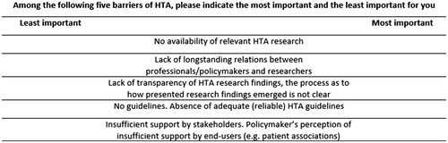
Table 1. Master lists of the barriers to the uptake of HTA.

Lack of timeliness. Gap between HTA research and policy-making regarding timeliness of research

Lack of longstanding relation between professionals/policy-makers and researchers

Lack of contact and interaction, among policy-makers, HTA researchers, and other stakeholders

No availability of relevant HTA research for policy-makers

No access to relevant HTA research (or poor dissemination) for policy-makers

Lack of financial resources to conduct relevant HTA research

Lack of qualified human resources to conduct or understand relevant HTA research within the policy organization

Absence of policy networks (or observatories that promote the joint efforts of researchers and policy-makers)

No guidelines. Absence of adequate (reliable) HTA guidelines

Lack of awareness, within the organization to the relevance of HTA

Lack of support, within the organization to the use of HTA

Lack of transparency of HTA research findings, i.e. the process as to how presented research findings emerged is not clear

Insufficient quality of HTA research findings: quality not in accord with scientific requirements

Lack of credibility of the HTA research findings (industry-sponsored studies)

Lack of consensus between HTA findings, existence of different and opposing recommendations

Limited generalizability of HTA studies to the policy-maker’s context

Uncertainty surrounding HTA results

Inadequate presentation format. HTA reports overly long, too theoretical or abounding in technical jargon

No explicit framework for decision making process, that uses HTA evidence

Insufficient support by stakeholders. Policy-maker's perception of insufficient support by end-users (e.g. patient associations)

Insufficient legal support. Lack of legal or legislative support for the use of HTA

Absence of appropriate incentives for the implementation of cost-effective interventions

Participants

A convenience sampling strategy was applied to recruit policy-makers (i.e. decision-makers and advisors on different levels) and HTA experts (i.e. PhD students and senior researchers in HTA) in all four countries. Potential participants were identified and recruited by in-country researchers through personal networks enriched with an internet search via HTA departments and institutes. All potential participants were approached by in-country investigators between November 2015 and May 2017 (i.e. Netherlands, n = 222; Germany, n = 365; France, n = 109; UK, n = 255). The Qualtrics system sent out e-mails which included a link to the survey, and randomly assigned each participant to one of the four versions of the questionnaire (each containing the 14 choice tasks) regarding the barriers to using HTA.

Analyses

Fully completed questionnaires were included in the analysis. Descriptive statistics were calculated to present demographic characteristics of the respondents. Data were analyzed using the five selected analysis methods: (1) count analysis, (2) multinomial logit, (3) mixed logit, (4) latent class analysis, and (5) hierarchical Bayes estimation. Resulting rankings were then compared among the methods, with the exception of the latent class analysis as this method characterizes unobserved, or latent, segments in the total group of participants, rather than yielding main effects for the total group. The respondent heterogeneity for the latent class analysis and the mixed logit model were then compared and discussed.

Count analysis

Count analysis is one of the simplest methods for analyzing BWS data, and is being used increasingly⁶. It is based on orthogonal assumption, and is limited to examining choice frequencies (on the sample level or on the individual level)^7,18. For each factor, the frequency of it being chosen as the best choice minus the frequency of it being chosen as the worst choice gives the best–worst score¹⁹. To standardize the score, this best–worst score of a factor is divided by the total number of occurrences of the factor in the sample and adjusted for the sample size⁷. The standardized best–worst score ranges between –1 and 1. For this study we used Microsoft Excel (2013)²⁰ to quantify the importance of each barrier, with a higher score indicating a higher level of perceived importance of the barrier.

Multinomial logit model

The multinomial logit model incorporates the logit procedure (where each factor has dual coding, best = 1 if the factor is chosen as most important, and best = 0 if otherwise; and worst = 1 if the factor is chosen as least important, and worst = 0 if otherwise) which yields propensity scores capturing the probability of a factor being present in a specific combination of factors⁷. Data analysis was conducted using Nlogit (version 5.0)²¹. Each factor is represented by a coefficient in a function, β, representing the relative preference (importance) of that factor, compared to a reference factor (i.e. based on the first barrier: “Lack of timeliness”)⁸. The relative preference (importance) of each factor can be seen as a measure of the strength and direction of preference for a particular factor relative to the common reference factor.

Mixed logit model

The mixed logit model accommodates preference heterogeneity, drawing on the assumption that parameters are distributed randomly in the population; the model captures heterogeneity by estimating the standard deviation of the parameter’s distribution²². Similar to the multinomial logit model, the factor’s coefficient β represents the relative preference (importance) for that factor, compared to a reference factor (i.e. barrier 1; “Lack of timeliness”). Next to the β, the mixed logit model incorporates a standard deviation term for each factor, η, capturing individual-specific unexplained variation around the mean. All factors were specified as random parameters and were drawn from a normal distribution using 500 Halton draws. Significant preference heterogeneity for the factor was concluded when its standard deviation term was significantly different from zero. Nlogit was used to conduct the analysis.

Latent class analysis

Latent class analysis was developed to characterize latent variables²³. When the use of observable socio-economic characteristics does not form homogeneous groups, latent class analysis may be useful to identify hidden heterogeneity among respondents^7,11. In order to identify potential latent segments, we ran different numbers of clusters with all 22 barriers using Nlogit. To determine (the number of) clusters, Akaike’s information criterion (AIC) and McFadden Pseudo R-squared (ρ²) were used. These are good and widely used indicators for model choice, where the model with the best fit has the lowest AIC and highest ρ² values^24,25.

Hierarchical Bayes estimation

Finally, we explored the hierarchical Bayes estimation. Using data at the individual level, a posteriori distributions were derived for the parameters⁷. Using Sawtooth Software’s SSI Web platform, the mean relative importance score (RIS) was calculated for each factor. Based on the raw coefficient of the preference function, re-scaled scores were estimated to represent the relative importance of the factors; when all factors are combined, the RIS for each individual sum up to 100, with a higher score indicating higher importance of the factor²⁶.

Results

Descriptive statistics

A total of 136 stakeholders completed the survey fully and were included in this analysis. The mean age of the participants who completed the survey was 45.2 years (SD =11.93); 52.2% were male. The final sample included 49 (36.0%), 31 (22.8%), 24 (17.6%), and 32 (23.5%) participants from the Netherlands, Germany, France, and the UK, respectively. Overall, there were 48 policy-makers (35.3%) and 88 HTA experts (64.7%), but the relevant proportions varied between countries (e.g. the Netherlands: 32.7% policy-makers; Germany; 67.7% policy-makers; France: 29.2% policy-makers; UK: 12.5% policy-makers)¹⁵.

Ranking of the factors for each analysis method

As shown in Table 2, four different analyses resulted in ranking the importance of the 22 barriers. The latent class analysis yielded rankings per latent segment only. Then, the rankings of the factors were compared to explore to what extent rankings differed between the methods for the count analysis, the multinomial logit and mixed logit models, and the hierarchical Bayes estimation (see Table 2).

Table 2. Comparison of rankings for each analysis method.

	Count analysis		MNL		MXL			HB
List of barriers	Ranking	BWS score	Ranking	β	Ranking	β	η	Ranking	RIS
No explicit framework for decision-making process	1	0.26	1	0.65**	1	0.77**	1.46**	1	7.63
Limited generalizability	2	0.23	2	0.58**	2	0.72**	0.23	2	6.92
Lack of consensus between HTA findings	3	0.13	3	0.26*	3	0.35*	1.19**	4	5.86
No availability of relevant HTA research	4	0.12	4	0.24	4	0.29	1.16**	3	6.00
Lack of qualified human resources	5	0.06	6	0.09	7	0.17	1.18**	7	4.98
Insufficient quality	6	0.06	5	0.10	6	0.17	1.10**	5	5.12
Lack of support, within the organization	7	0.05	9	0.00	10	0.03	1.12**	10	4.78
Lack of awareness, within the organization	8	0.05	8	0.02	11	0.01	0.99**	8	4.83
Uncertainty surrounding HTA results	9	0.04	11	–0.03	9	0.05	1.29**	9	4.81
Lack of transparency of HTA research findings	10	0.03	7	0.05	8	0.05	0.38	12	4.46
Lack of timeliness	11	0.02	10	0.00	12	0.00	0.00	11	4.74
No access to relevant HTA research	12	0.01	12	–0.09	13	–0.06	1.30**	6	5.02
Lack of credibility	13	0.00	13	–0.10	14	–0.13	0.46	15	3.95
Insufficient support by stakeholders	14	–0.02	14	–0.20	15	–0.25	0.99**	14	4.09
Absence of appropriate incentives	15	–0.05	16	–0.28**	5	0.27	1.66**	13	4.20
Lack of contact and interaction	16	–0.05	15	–0.25**	16	–0.31*	0.91**	16	3.81
Lack of financial resources	17	–0.06	17	–0.29**	17	–0.45**	1.07**	17	3.59
Insufficient legal support	18	–0.13	18	–0.46**	19	–0.56**	1.40**	18	3.52
No guidelines	19	–0.15	19	–0.52**	18	–0.54**	1.32**	20	2.98
Lack of longstanding relation	20	–0.16	20	−0.54**	20	–0.64**	1.62**	19	3.29
Inadequate presentation format	21	–0.18	21	−0.62**	21	–0.80**	1.48**	21	2.89
Absence of policy networks	22	–0.19	22	–0.66**	22	–0.92**	0.95**	22	2.51

List of barriers are ordered according to the count analysis ranking. The ranking indicates the position of each barrier in each of the statistical methods (e.g. “Lack of consensus between HTA findings” was ranked position three in the count analysis, MNL and MXL, and position four in the HB analysis).

Abbreviations: HB, Hierarchical Bayes ranking; RIS, Relative Importance Score; MNL, Multinomial Logit ranking; MXL, Mixed Logit ranking; β, relative preference compared to the reference factor; η, standard deviation term for the factor.

* p < 0.05;

** p < 0.01.

Comparing the five factors ranked as best, rankings showed similar results between these methods. The factors “No explicit framework for decision-making process”, “Limited generalizability”, “Lack of consensus between HTA findings”, and “No availability of relevant HTA research” were all ranked in the top four of the different analyses, while the fifth (“Lack of qualified human resources”) was similarly ranked across the analyses, i.e. between position 5 and 7. In terms of the five factors ranked as worst, the barriers “Insufficient legal support”, “No guidelines”, “Lack of longstanding relation”, “Inadequate presentation format’, and “Absence of policy networks” were all ranked in the top five of the least important barriers. Overall, rankings were similar, and the extremes (best: “No explicit framework for decision-making process”; worst: “Absence of policy networks”) were identical across the analysis methods.

Analysis methods handling respondent heterogeneity

In the latent class analysis, the model with five clusters had the best fit (AIC =9,249.30 and ρ² = 0.25). In these five models, between 8 and 16 coefficients were significantly different from zero, representing the reference factor (p < 0.05). The estimated latent class probabilities for each cluster were 0.39, 0.14, 0.13, 0.11, and 0.23 (p < 0.01), respectively. The rankings per cluster showed preference differences between latent segments. For instance, the factor “No explicit framework for decision-making process” was ranked 5, 15, 8, 1, 1, in clusters 1, 2, 3, 4, and 5, respectively (see Table 3).

Table 3. Latent class analysis. Latent clusters and comparison of rankings.

	C1		C2		C3		C4		C5
Barriers	R	β	R	β	R	β	R	β	R	β
1. No explicit framework for decision-making process	5	1.08**	15	–0.88*	8	0.92*	1	0.91	1	0.79*
2. Limited generalizability	3	1.20**	3	0.67	9	0.78	7	–0.57	7	–0.34
3. Lack of consensus between HTA findings	11	0.51	2	0.74	7	1.13**	13	–1.21*	8	–0.79*
4. No availability of relevant HTA research	2	1.31**	6	0.04	17	0.21	8	–0.74	20	–1.85**
5. Lack of qualified human resources	10	0.68*	21	–1.79**	3	2.14**	6	–0.49	15	–1.28**
6. Insufficient quality	1	1.37**	9	–0.14	14	0.43	16	–1.70**	18	–1.57**
7. Lack of support, within the organization	13	0.14	20	–1.56**	5	1.40**	4	–0.16	5	–0.08
8. Lack of awareness, within the organization	9	0.72*	19	–1.38**	11	0.65	2	0.41	9	–0.82*
9. Uncertainty surrounding HTA results	14	0.07	1	1.13*	20	–0.14	14	–1.27*	10	–1.07**
10. Lack of transparency of HTA research findings	7	0.75**	5	0.14	12	0.62	17	–1.87**	13	–1.16**
11. Lack of timeliness (ref)	16	0.00	7	0.00	19	0.00	3	0.00	4	0.00
12. No access to relevant HTA research	4	1.11**	8	–0.02	16	0.26	12	–1.20*	22	–2.41**
13. Lack of credibility	6	0.78**	12	–0.46	13	0.45	19	–2.06**	14	–1.21**
14. Insufficient support by stakeholders	19	–0.47	10	–0.20	6	1.35**	18	–1.94**	6	–0.08
15. Absence of appropriate incentives	17	–0.23	11	–0.31	18	0.00	21	–2.40**	3	0.20
16. Lack of contact and interaction	20	–0.94**	4	0.33	1	2.85**	10	–1.00	19	–1.58**
17. Lack of financial resources	15	0.02	17	–1.17*	10	0.72	11	–1.16	12	–1.15**
18. Insufficient legal support	12	0.16	22	–2.32**	15	0.36	22	–4.25**	2	0.36
19. No guidelines	8	0.73**	18	–1.26	22	–0.31	20	–2.21**	21	–2.10**
20. Lack of longstanding relation	22	–1.37**	13	–0.47	4	2.06**	9	–0.83	11	–1.07**
21. Inadequate presentation format	18	–0.46	14	–0.87*	21	–0.29	5	–0.29	17	–1.55**
22. Absence of policy networks	21	–1.17**	16	–1.01*	2	2.16**	15	–1.69**	16	–1.39**
Latent class probability		0.39**		0.14**		0.13**		0.11**		0.23**

List of barriers are ordered according to the count analysis ranking of Table 2 (e.g. barrier “Lack of timeliness” is ranked 16^th in C1).

Abbreviations: C1, C2, C3, C4, C5, Class 1, Class 2, Class 3, Class 4, Class 5; R, ranking.

* p < 0.05;

** p < 0.01.

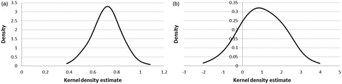
For the mixed logit model, significant preference heterogeneity was found for all factors (when their standard deviation term was significantly different from zero), with the exception of three factors (excluding the reference factor): “Limited generalizability”, “Lack of awareness, within the organization”, and “Insufficient support by stakeholders”. The mixed logit model, therefore, suggests that the preferences for factors differ among respondents. The respondent heterogeneity can be reflected in the kernel densities (see Figure 2), which provide a visual representation of the potential variation in preferences for each of the factors. Figure 2 illustrates, for example, that for two factors with a similar average score (i.e. “Limited generalizability” and “No explicit framework for decision-making process”), variation between respondents differs markedly, with almost no variation for “Limited generalizability” (Figure 2a), and an important variation for “No explicit framework for decision-making process” (Figure 2b).

Figure 2. Kernel density estimate for “Limited generalizability” (a) and “No explicit framework for decision-making process” (b).

Discussion

This study aimed to compare five different object case BWS analysis methods: (1) count analysis, (2) multinomial logit, (3) mixed logit, (4) latent class analysis, and (5) hierarchical Bayes estimation. The study aims at being a step towards the better understanding of the different existing analysis methods, as recently demanded by the International Society for Pharmacoeconomics and Outcomes Research (ISPOR) for conjoint analyses in general²⁷.

Overall, the five statistical analyses resulted in similar rankings, in particular in the extreme ends of rankings (five best and worst factors). Methods based on frequency (i.e. count analysis and hierarchical Bayes estimation) yielded similar rankings to the other approaches. Findings indicate that, albeit not allowing for comparability of results across different studies⁷, the more simplistic, summative, methods like count analysis may be valid and accessible methods for healthcare researchers conducting BWS²⁸. Previous BWS applications incorporating multiple methods (i.e. in addition to count analysis) to analyze BWS data revealed similar rankings^29,30. The accessibility of the count analysis is also reflected in its increasing usage in BWS applications⁶. At the same time, in comparison with count analysis, an advantage of hierarchical Bayes estimation is that it may yield reliable individual best–worst values even in small samples⁷.

An argument for using the latent class model or the mixed logit model is that these models provide additional information on whether the preference for (importance of) a factor differs between respondents. This may be of additional interest from a clinical or policy perspective³¹. If one is interested in (also) identifying heterogeneity between respondents, the mixed logit model provides information on whether one can conclude on preference heterogeneity as a factor. In addition to revealing the respondent heterogeneity of individual factors, latent class analysis identifies latent segments (meaning underlying clusters), classifies participants in clusters, and yields latent class probabilities for each cluster. In our analysis, substantial heterogeneity was observed in the preferences of the latent classes, meaning that different factors may be perceived as most important by different subgroups, and this could have been revealed only by the latent class or the mixed logit model.

According to the ISPOR Conjoint Analysis Good Research Practices³¹, different statistical analysis methods are acceptable and may be used in conjoint analyses. While the current study is, to our knowledge, the first to make a comprehensive comparison of alternative methods for an object case BWS, the mixed logit and multinomial logit approaches are also relevant statistical methods for other types of DCEs and BWS formats³¹.

Our study has potential limitations. One is that a variety of statistical software packages and different versions were used to perform relevant BWS analyses^6,32, which may potentially add to differences in the rankings between the analyses in the study. Also reflected in best–worst scaling studies in healthcare⁶, SAS, Nlogit, Stata, R, and Latent Gold are interesting programs to be explored, as these have been applied in best–worst scaling studies in the field. Future research may shed light on the different assumptions and findings underlying the variety of existing software for analyzing BWS data. Therefore, in line with relevant ISPOR recommendations for DCEs²⁷, it is important to report on the specific software program used for the analysis, to enhance transparency and clarity. Many previously published BWS studies did not report such details⁶. Another limitation of this study may be that a comparison of different analysis methods was conducted for object case BWS only. Findings are, therefore, not necessarily generalizable to other BWS formats, i.e. the BWS profile and the BWS multi-profile case²⁸, or to other conjoint analyses methods. Further work using other databases would need to be done to confirm our findings, as study design and context may potentially affect the performance of the analytical methods (e.g. sample size and number of factors).

Conclusion

To the best of our knowledge, this paper is the first to comprehensively test the comparability of commonly used analysis methods for BWS using data from a case study that quantifies the importance of barriers to the usage of HTA in several European countries. Findings revealed similar rankings, in particular in the extremes, between the analysis methods. This could suggest that the simpler analysis method, count analysis, may be a valid and sufficient approach for healthcare researchers to analyze data for the object case BWS, when one is interested only in analyzing preference ranking. However, more complex methods (i.e. multinomial and mixed logit models) may reveal additional information on whether preferences differ among respondents. The mixed logit model and latent class analysis reveal the respondent heterogeneity of the BWS data.

Transparency

Declaration of funding

No funding was received for this study.

Declaration of financial/other relationships

There are no financial or other relationships to be declared. KLC received financial support for his research stay at the Department of Health Economics, Center for Public Health, Medical University of Vienna through the “Erasmus + staff mobility grant”. The authors declare that they have no competing interests. JME peer reviewers on this manuscript have no relevant financial or other relationships to disclose.

Acknowledgements

We are indebted to Pierre Levy, Teresa Jones, Subhash Pokhrel, Marion Danner, Jana Wentlandt, and Laura Knufinke for the country-specific survey preparation, recruitment, and data collection. The views expressed and any errors in this article are those of the authors.

References

- Bridges JF, Jones C. Patient-based health technology assessment: a vision of the future. Int J Technol Assess Health Care. 2007;23(1):30–35.
- Ryan M, Gerard K. Using discrete choice experiments to value health care programmes: current practice and future research reflections. Appl Health Econ Health Policy. 2003;2(1):55–64.
- Janz NK, Wren PA, Copeland LA, et al. Patient-physician concordance: preferences, perceptions, and factors influencing the breast cancer surgical decision. J Clin Oncol. 2004;22(15):3091–3098.
- Facey K, Boivin A, Gracia J, et al. Patients' perspectives in health technology assessment: a route to robust evidence and fair deliberation. Int J Technol Assess Health Care. 2010;26(03):334–340.
- Green PE, Srinivasan V. Conjoint analysis in consumer research: issues and outlook. J Consumer Research. 1978;5(2):103–123.
- Cheung KL, Wijnen BF, Hollin IL, et al. Using best-worst scaling to investigate preferences in health care. Pharmacoeconomics. 2016;34(12):1195–1209.
- Mühlbacher AC, Kaczynski A, Zweifel P, et al. Experimental measurement of preferences in health and healthcare using best-worst scaling: an overview. Health Econ Rev. 2016;6(1):1–14.
- Flynn TN, Louviere JJ, Peters TJ, et al. Best-worst scaling: what it can do for health care research and how to do it. J Health Econ. 2007;26(1):171–189.
- Marley AA, Louviere JJ. Some probabilistic models of best, worst, and best-worst choices. J Math Psychol. 2005;49(6):464–480.
- Louviere JJ, Flynn TN, Marley A. Best-worst scaling: Theory, methods and applications. Cambridge (UK): Cambridge University Press; 2015.
- Cohen S, editor. Maximum difference scaling: improved measures of importance and preference for segmentation. Sawtooth Software Conference Proceedings, Sawtooth Software Inc. 2003;530:61–74.
- Flynn TN, Louviere JJ, Peters TJ, et al. Estimating preferences for a dermatology consultation using best-worst scaling: comparison of various methods of analysis. BMC Med Res Methodol. 2008;8(1):76.
- Prosser LA. Statistical methods for the analysis of discrete-choice experiments: a report of the ISPOR conjoint analysis good research practices task force. Value Health. 2016;19(4):300–315.
- Cheung KL, Evers S, De Vries H, et al. Most important barriers and facilitators regarding the use of health technology assessment. Int J Technol Assess Health Care. 2017;33(2):1–9.
- Cheung KL, Evers, S, De Vries H, et al. Most important barriers and facilitators of HTA usage in decision-making in Europe. Expert Rev Pharmacoecon Outcomes Res. 2018:18(3):297–304.
- Sawtooth Software. Provo, Utah, USA; 2017. Available at: https://www.sawtoothsoftware.com
- Qualtrics Research Suite. Provo, Utah, USA; 2017. Available at: https://www.qualtrics.com
- Louviere JJ, Flynn TN. Using best-worst scaling choice experiments to measure public perceptions and preferences for healthcare reform in Australia. Patient. 2010;3(4):275–283.
- Coltman TR, Devinney TM, Keating BW. Best–worst scaling approach to predict customer choice for 3PL services. J Business Logistics. 2011;32(2):139–152.
- Microsoft Excel; 2013. Available at: https://office.microsoft.com/en-us/excel
- NLogit, Economic Software Inc. 2017. Available at: https://www.limdep.com
- Lancsar E, Louviere J. Conducting discrete choice experiments to inform healthcare decision making: a user's guide. Pharmacoeconomics. 2008;26(8):661–677.
- Schreiber JB. Latent class analysis: an example for reporting results. Res Social Adm Pharm . 2017;13(6):1196–1201.
- Bozdogan H. Model selection and Akaike’s information criterion (AIC): the general theory and its analytical extensions. Psychometrika. 1987;52(3):345–370.
- McFadden D. Quantitative methods for analysing travel behaviour of individuals: some recent developments. In: Hensher DA, Stopher PR, editors. Behavioural Travel Modelling. London: Croom Helm; 1978. p 279–318.
- Orme B. Hierarchical Bayes: why all the attention? QMRR. 2000;14(3):16–63.
- Hauber AB, González JM, Groothuis-Oudshoorn CG, et al. Statistical methods for the analysis of discrete choice experiments: a report of the ISPOR Conjoint Analysis Good Research Practices Task Force. Value Health. 2016;19(4):300–315.
- Flynn TN. Valuing citizen and patient preferences in health: recent developments in three types of best–worst scaling. Expert Rev Pharmacoecon Outcomes Res. 2010;10(3):259–267.
- Gallego G, Bridges JF, Flynn T, et al. Using best-worst scaling in horizon scanning for hepatocellular carcinoma technologies. Int J Technol Assess Health Care. 2012;28(3):339–346.
- Marti J. A best-worst scaling survey of adolescents' level of concern for health and non-health consequences of smoking. Soc Sci Med. 2012;75(1):87–97.
- Bridges JF, Hauber AB, Marshall D, et al. Conjoint analysis applications in health—a checklist: a report of the ISPOR Good Research Practices for Conjoint Analysis Task Force. Value Health. 2011;14(4):403–413.
- Lancsar E, Fiebig DG, Hole AR. Discrete choice experiments: a guide to model specification, estimation and software. Pharmacoeconomics. 2017;35(7):697–716.